Development of a Model for the Estimation of the Energy Consumption Associated with the Transportation of CO₂ in Pipelines

Abstract

All Carbon Capture and Storage (CCS) projects require the transportation of CO₂ from a source to a storage location. Although, a compressor and a large diameter pipeline is the normal method used to achieve this, liquefaction, shipping and pumping is sometimes attractive. Identifying the economic optimum is important for all CCS projects, minimizing energy consumption is also important because it corresponds to a resource efficiency in fossil-fuel based projects. This article describes the development and validation of a model that estimates the energy consumption associate with CO₂ transportation using the geographic location of the source and the reservoir to incorporate ambient temperature and bathymetry data. The results of the validation work show an average absolute temperature and pressure error less than 1 °C and 1 bar compared to a reference model. The model has been developed using openly accessible data and is made available in a repository for open research data.

1. Introduction

There are currently 19 large-scale Carbon Capture and Storage (CCS) projects in operation worldwide [1], but to achieve the level of CO₂ emissions in the International Energy Agency’s Sustainable Development Goals (SDGs) the number of industrial scale facilities will need to increase to more than 2000 by 2040 [2]. Each of these projects requires the transportation of CO₂ from a point of origin to a storage location and, since the transportation distance is often significant, over 200,000 km of CO₂ pipelines will be required by 2050 by CCS projects [3]. Although the majority of CO₂ is likely to be transported using pipelines, the success of many future CCS projects will depend on transportation using ships. For example, the Northern Lights Project, which will be one of the first full-chain projects in Europe [4], is based on ship transportation of CO₂ from a source to a hub where a sub-sea pipeline will then connect to the storage location in the Norwegian Sea.

Research supporting the design of CO₂ transportation processes has been widely published. A particular focus has been CO₂ mixture properties in high-pressure pipelines [5,6,7,8,9], but many other aspects of CO₂ pipeline design have been studied, including heat transfer [10,11,12], transient flow behavior [13] and economic optimization [14,15,16], to name some examples. Although less research has focused specifically on ship-based transportation, there are still a large number of studies looking at both technical and economic aspects of CO₂ shipping [17,18,19], and a particular focus being the energy consumption associated with the compression and liquefaction processes [20,21,22,23,24,25].

Figure 1 presents an illustration of the CCS value chain. The illustration indicates that the break-point between the capture and transportation is not always clear-cut, reflecting the fact that some capture processes produce CO₂ at elevated pressure. Based on this, and because the capture process is normally the main contribution to overall energy consumption, the full chain, rather than transportation in isolation, is often the focus of research work. However, the transport energy consumption and the capture unit energy consumption are often independent: One capture option can having multiple possible transportation possibilities with differing energy consumption.

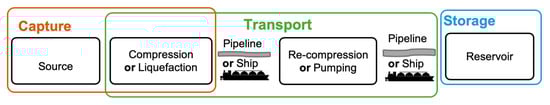
Figure 1. Simplified Illustration of a Typical CCS Value Chain.

In the context of the economic basis for specific CCS projects the selection of the optimum transportation alternative is normally studied. For example, Jakobsen, et al. studies the transportation alternatives associated with the Norcem Brevik cement plant CCS project [26]. Also, to support the economic assessment of CCS projects in general, tools for modelling full CCS chains have been developed that allow comparison of different transportation cases, for example Jakobsen, et al. [27]. Studies have also been conducted in the identification of a more general economic trade-off distance between shipping and pipelines, for example Mallon, et al. [28].

The purpose of the model presented here, in contrast to other work, is to allow the study and comparison of different CO₂ transportation chains on the basis of their energy consumption. The purpose of this article is to present details of how the model was developed and tested.

The model presented here is currently limited to pre- and post-combustion CO₂ stream composition and transportation scenarios in the North, Norwegian and Barents Seas. The inclusion of performance data for different CO₂ sources is planned for future development. The intended use of the model is not as a replacement or competitor to other modelling approaches, but as a tool that enable a perspective on CCS project alternatives focused on energy consumption. Case studies and sensitivity analysis using the mode will be developed and presented as part of future work.

2. Methods

The model described here was developed in Matlab [29] to take advantage of several useful built-in functions, particularly those available via the Mapping and Curve Fitting toolboxes, both of which are required to allow the model to run. The model is built-up from a set of ‘functions’ that can be called using a ‘script’ called Main. In the following description all of the files that make up the model are referred to using italics to highlight their significance. All of the data required for the model to run is incorporated into the model. A summary of the functions that make-up the model and the basis data which is used is provided in Table 1.

Table 1. Summary of Functions and Basis Data.

Functions	Description	Basis Data	Description
CO2TransModel	Main function taking input data from Case, passes data to other functions and formats the results.	Case	The description of the CCS transport scenario considered. User input.
PipeProf	Calculated the elevation profile based on Case.	Bath SSTdata	Bathymetry basis data Sea temperature basis data
PressProf	Calculates pressure and temperature profiles based on PipeProf & stream properties data.	Post Pre Oxy *	Stream properties data including: compositions, density data, critical constants, dew-point, bubble-point, JT coefficient, heat capacity.
PressureDrop	Pressure drop used in PressProf.
fFact	Friction factor used in PressureDrop.
Visc	Viscosity calculation.
TransEnergy	Calculates energy consumption for compression OR liquefaction and pumping based on PressProf and the SSTdata.	CompPost CompPre CompOxy * Liq_Power	Data relating to the energy consumption for compression, liquefaction and pumping of CO2 at different pressure and temperature conditions.

* Data available in the model, but not implemented in the TransEnergy calculations.

A description of each the model input, calculation methods, basis data and outputs is presented below under several headings.

2.1. Case Defenition

An interface to the model is provided in the script Main, which contains guidance on defining the basis for running the model. The basis for any particular case is stored as variables in a ‘structure’ called Case. A summary of the required input data for Case is provided in Table 2.

Table 2. Summary of Model Input Parameters.

Name	Description
POI	Geographic reference points (decimal degrees) describing the pipeline route **
Opt	Transport type: 1 = pipeline *; 2 = ship
LiqLoc	Location of the liquefaction process (Opt = 2 only) in decimal degrees
WH_loc	Wellhead location: 0 = sub-sea * and 1 = surface wellheads
Res_Depth	Reservoir depth in meters **
Pipe_e	Roughness in µm, default is 15 µm
Stream	‘Post’ *, ‘Pre’ or ‘Oxy’ composition
T_inlet	Pipeline inlet temperature
U	Heat transfer coefficient, default value is 6 W/m2-K
Flow	Case flowrate in Mtpa **
T_sea	Sea water temperature in °C ***
Pipe_prof	Elevation profile ***

* Default option in the model ** Default is Melkøya based on *** Optional user input: replaces default methods.

CO₂ originating from different emission sources will often have different composition. This impacts on the phase behavior of the mixture and pipeline operating conditions. To take account of this in the model and to maintain consistency with earlier work, three CO₂ mixtures can be selected in the model by specifying either ‘Post’, ‘Pre’ or ‘Oxy’ as the Stream in Case. These stream alternatives represent a post-combustion capture process from flue gas using a chemical solvent, a pre-combustion capture process from syngas (also using physical solvent) and an oxyfuel flue gas originating from an oxyfuel purification unit. Table 3 summarizes the composition of these streams.

Table 3. CO₂ Mixture Compositions.

Component	Post	Pre	Oxyfuel
CO2 mole %	99.99	99.50	96.16
N2 mole %	0.01	-	2.45
CH4 mole %	-	0.50	-
Ar mole %	-	-	0.96
O2 mole %	-	-	0.43

Several example cases are made available for use with the model and can be called using Main. Alternatively, the user can simply create their own Case structure using the parameters from Table 2, or they can simply run Main without alteration, which returns results with the default parameters specified in Case.

Within Main plotting and saving behavior can also be specified using a parameter called Plot, which defines the level of plot data generated: 0 = no plots, 1 = simple plots and 2 = all plots, and a parameter called Save, which can be set to either 1 = save results, or 0 = no save. Running Main calls the function CO2TransModel, which subsequently calls the other functions listed in Table 1.

2.2. Pipeline Elevation Profile and Sea Temperature

Pressure changes in CO₂ pipelines occur due to frictional loss, elevation change and acceleration. As the latter is very small compared to the others it is excluded from the present model. Both of the other effects must be adequately accounted for to ensure an accurate model. Frictional pressure loss varies with pipeline length while changes in static pressure depend on pipeline elevation. Length and elevation data is used by the model in the form of the pipeline profile called Pipe_prof, which is generated using the PipeProf function and basis data from Case. Within PipeProf the profile is calculated using the POI defined in Case and the basis data defined in Bath.

The basis for the data stored in Bath is GEBCO’s gridded bathymetric data set: GEBCO 2019 [30]. The data from the dataset was processed after downloading: the data in ‘geotiff’ format was converted to a georeferenced data grid using the ‘geotiffread’ function and then it was down sized to 20% using the built-in ‘resizem’ function. Data is currently only stored for the North, Norwegain and Barents Sea: latitude 47° N to 75° N and −10° E to 30° E.

Within PipeProf a profile is generated using the mapprofile function and the POI defined in Case, which must be given in decimal degrees. The profile generated reflects the contours of the seabed and not necessarily a realistic pipeline route, which would be designed to avoid abrupt changes in direction. To reflect this, the raw profile data is smoothed before it is used in the pressure drop calculations.

To ensure that the method described above gives a realistic result for the pipeline profile, published profile data from the Melkøya CO₂ pipeline [31] was used in a qualitative validation exercise, which is presented in Figure 2. The method used in the validation exercise was to define a pipeline based on the information contained in [31] and then to automatically generate a pipeline profile from the bathymetry data stored in the model. The modelled pipeline elevation profile could then be compared to the pipeline elevation profile presented in [31] to check consistency. The results of this comparison as illustrated in Figure 2.

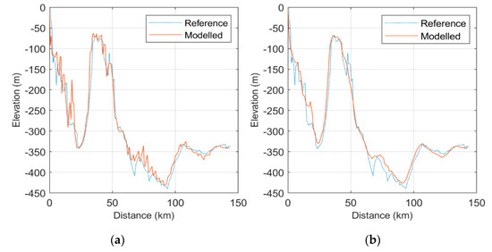
Figure 2. Elevation Profile Comparison Between Reference Data for Melkøya; [31] and (a) Modelled Profile with no Smoothing; (b) Profile with Smoothing.

To allow the comparison of pipeline operating conditions in different geographic locations the model calculates the average sea temperature for the pipeline, $T_{\mathrm{sea}}$, based on Sea Surface Temperature (SST) data for the 10 year period April 2009 to April 2019. The data was obtained from Japan Meteorological Association (JMA) [32] and is stored in the model as the file SSTdata.

In the development of the model, raw data from JMA was converted to NetCFD format for easy use, and trimmed to cover only the area of interest. Monthly averaged data was then used to determine the mean SST value at each grid point. A value of SST equal to mean plus two standard deviations was then calculated to set a realistic maximum pipeline design operating temperature that reflects 97.5% of the monthly averaged data.

In reality, the temperature of the seawater below the surface will normally be several degrees lower than SST. This reduction in temperature below SST is difficult to generalize, and is therefore, not used in the model. To allow flexibility, the option to manually set a value for $T_{\mathrm{sea}}$ is provided via the parameter $T_{\mathrm{sea}}$ in Case.

2.3. Pipeline Pressure and Temperature Profiles

Both the pipeline pressure and temperature profiles are generated by the PressProf function which uses the results from PipeProf and data for the Stream specified in Case. The procedure contained in PressProf is a numerical stepwise approach to the calculation of the pipeline pressure profile,

$$P_{\mathrm{out}}=P_{\mathrm{in}}-\sum \left(∆P_n^f-∆P_n^s\right),$$

(1)

where$P_{\mathrm{out}}$ is the pipeline outlet pressure,$P_{\mathrm{in}}$ is the pipeline inlet pressure, $∆P_n^f$ is the frictional pressure drop for the element n in the pipeline and $∆P_n^s$ is the static pressure change for elmenet n. The calculation methods associated with static and frictional pressure change are detailed under later headings.

The calculation procedure for $P_{\mathrm{out}}$ begins with an estimate for $P_{\mathrm{in}}$ and continues stepwise with the pressure in each element ‘n’ calculated based on the pressure in the previous element. When the pipeline pressure calculation has been completed, the calculated value of $P_{\mathrm{out}}$ is compared to the WHP and the minimum allowable pipeline pressure along the full length of the pipeline, $P_n^{\min }$, and a correction is made to the estimated value of $P_{\mathrm{in}}$:

$$C=\max \left(\mathrm{WHP}-P_{out} \& P_n^{\min }-P_n\right),$$

(2)

$$\mathrm{and} P_{\mathrm{in}}=P_{\mathrm{in}}+C,$$

(3)

where C is a correction factor used in the calculation algorithm. The pressure drop calculation then continues iteratively until the absolute value of C is less than 1 bar. The calculation of WHP and $P_n^{\min }$ is described under the next two headings.

2.3.1. Well Head Pressure

Studies such as that of Maldal [33] and Shi et al. [34] illustrate that CO₂ reservoir pressure will normally change substantially over time, varying with reservoir conditions and operating parameters such as flowrate. This makes the selection of a representative modelling basis for WHP complicated. The approach taken in this study was, therefore, to assess the range of likely reservoir pressure conditions across the lifespan of storage reservoir from limiting cases. For example, Vishal et al. [35] state that “Depending on the national regulatory, maximum allowed [over] pressure generally corresponds to the 50% of the initial hydrostatic pressure or the 60% of initial lithostatic pressure at the top of the storage formation”. Accordingly, the model present results for three cases where the reservoir pressure is set at 10%, 30% and 50% above initial hydrostatic pressure, which is calculated from the Res_Depth parameter in Case,

$$P_R={\rho }_w·h·g·{10}^{-5},$$

(4)

where $P_R$ (bar) is the reservoir pressure, ${\rho }_w$ is the density of water (kg/m³) and $h$ is the depth of the reservoir (m) and $g$ is the gravitational constant (m/s²).

Frictional pressure loss in the pipework associated with the well depends on the length of the well, its diameter and the injection rate, which in-turn depends on the number of injection wells. In this work, for simplicity, the wellhead frictional pressure drop has been based on the Norsok Standard, P-100, which calls for a pressure drop of 0.11–0.27 bar/100 m for wells operating 35–138 barg. WHP is calculated by dividing the well pipework into 100 elements and summating the static head change and frictional pressure loss in each element,

$$\mathrm{WHP}=P_{R}R+{\sum }_{i=1}^{100}{h}_i\left({\rho }_i·g·{10}^{-5}-∆P_W^f{10}^{-2}\right),$$

(5)

where $R$ is the overpressure ratio (1.1, 1.3 and 1.5 being the default values in the model), $h_i$ is the height of element i in the well pipework, ${\rho }_n$ is the density of the CO₂ mixture in element (kg/m³) and $∆P_W^f$ is a constant frictional loss = 0.15 bar/100 m for the pipework associated with the well(s).

2.3.2. Minimum Pipeline Operating Pressure

CO₂ pipelines are often designed based on a minimum operating pressure that is set at a margin above the critical pressure of the CO₂ mixture present in the pipeline [3,14,36], as illustrated below by the green dashed line in Figure 3. The purpose this is to avoid a situation where a pipeline operating in the supercritical region cools to conditions close to the critical point—where density can be difficult to predict—or, worse still, where pipelines operating in the gas phase cool leading to condensation. However, sub-sea pipelines located in the North, Norwegian and Barents Sea can be expected to operate with CO₂ in the dense phase, i.e., well below the critical temperature of CO₂ (31 °C). Under these conditions, phase change can be avoided by specifying a minimum approach to the bubble point curve as illustrated by the blue dashed line in Figure 3.

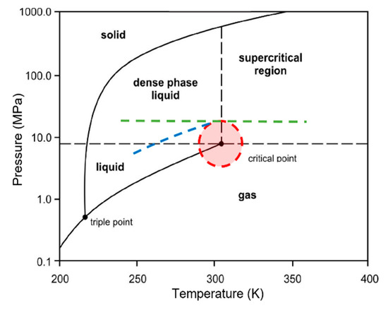
Figure 3. Illustration of Pipeline Operational Limits.

The model calculates the minimum operating pressure for each element in the pipeline as part of the pressure profile calculations in the PressProf function using a 10 bar margin to the bubble point pressure,

$$P_n^{\min }=P_n^{BP}+10 \mathrm{bar}$$

(6)

where $P_n^{\min }$ is the minimum operating press in element n and $P_n^{BP}$ is the bubble point pressure of the mixture in the pipeline at element n. Accurate prediction of the $P_n^{BP}$ of each CO₂ mixture is important to the specification of $P_n^{\min }$ and to ensure this, bubble point data from the TREND properties package [7] is used as the basis for the model. This basis data is stored in the files Post, Pre and Oxy as a set of gridded interpolation data.

2.3.3. Pipeline Diameter Selection

Several studies have presented methods for determining the optimim diameter for CO₂ pipelines [14,15,16], which is normally based on minimising costs. Others have proposed that “the smallest diameter which ensures that pressure drops are lower than the maximum allowable pressure is the cost-optimal diameter …” [37], but this only transfers the determination of optimum diameter to that of the determination of the maximum allowable pressure, which has been suggested to lie between 15.3 and 20 MPa [5,15,38,39]. The approach adopted in the model is, therefore, to obviate the difficulties associated with identifying optimum diameter by presenting results for a range of suitable diameters. The range used in a particular case is defined using a minimum inside diameter, $D_{\mathrm{ID}}^{\min }$, and the next three larger standard pipe sizes.

$D_{\mathrm{ID}}^{\min }$ is calculated using an erosional velocity limit, $u_e$, the minimum gas density in the pipeline, ${\rho }_{\min }$, and the parameter Flow from the model input parameters,

$$D_{\mathrm{ID}}^{\min }=\sqrt{\frac{4·m}{\pi ·{\rho }_{\min }·u_e}}$$

(7)

where $m$ is the mass flow in the pipeline (kg/s) based on the parameter Flow from Case. The erosional velocity limit is, in turn, calculated based on the formula given in API 14C and the factor ‘c’ taken as 100 for continuous flow [3],

$$u_e=0.82 \mathrm{c}/\surd {\rho }_{\min }$$

(8)

where the minimum gas density, ${\rho }_{\min }$, is calculated using the worst case for all minimum operating pressure conditions along the pipeline and the minimum SST.

The three standard pipe sizes that lie above $D_{\mathrm{ID}}^{\min }$ are based on 2 inch intervals between the standard pipe sizes. Early testing of the model confirmed that this approach covers all of the sizes that would normally be of interest for study purposes.

The density of the CO₂ mixture is used in several of the calculations carried out by the model and, therefore, accurate prediction at different pressure and temperature conditions is important. To ensure this, density data from the TREND [7] properties package is stored for each of the streams in the files Post, Pre and Oxy as a set of gridded interpolation data.

2.3.4. Calculation of Frictional and Static Pressure Changes

Frictional pressure drop, $∆P_n^f$, is calculated in Press_prof using the Darcy–Weisbach equation:

$$∆P_n^f=2f_F\frac{L_n}{D_{\mathrm{ID}}}{\rho }_n^{\mathrm{av}}{u}_n^2$$

(9)

where $f_F$ is the Fanning friction factor calculated using ${\rho }_n^{\mathrm{av}}$, $L_n$ is the length of element n, $D_{\mathrm{ID}}$ is the inside diameter of the pipeline (4 cases), ${\rho }_n^{\mathrm{av}}$ is the average density in element n and $u_n$ is the average velocity in element n, which is also calculated using ${\rho }_n^{\mathrm{av}}$.

The calculation of ${\rho }_n^{\mathrm{av}}$ is based on the assumption that, although $∆P_n^f$ is generally small for short $L_n$, the static pressure change, $∆P_n^s$, can be significant when the elevation change is also significant. Accordingly, the average pressure and density are estimated prior to conducting the pressure drop calculation to improve accuracy using a simple linear average,

$$P_n^{\mathrm{av}}=\frac{1}{2}[P_{n-1}+(P_{n-1}+{\rho }_{n-1}{}_{ }g E{l}_n)]$$

(10)

where $E{l}_n$ is the elevation change for the n^th element in the pipeline and ${\rho }_{n-1}$ is the density for the preceding pipeline segment n − 1, which is calculated as a function of pressure and temperature.

The static pressure loss in each pipeline segment is calculated using the average density:

$$∆P_n^s={\rho }_n^{\mathrm{av}}g E{l}_n.$$

(11)

The pressure drop calculations are made step-by-step alongside the temperature profile calculations for the full length of the pipeline. Temperature profile calculations are described under a separate heading.

2.3.5. Pipeline Roughness and Friction Factor

Pipeline roughness and friction factor have an important impact on pressure drop. In common with other studies [14,15], the model described here uses the Zirang and Sylverster equation [40] to estimate the Fanning friction factor, $f_F$, which has been shown by Winning and Coole [41] to give good accuracy,

$$\frac{1}{\sqrt{f_F}}=-4\log \left\{\frac{e/D_{\mathrm{ID}}}{3.7}-\frac{5.02}{{\mathrm{Re}}_n}\log \left[\mathrm{A}\right]\right\}$$

(12)

$$\mathrm{A}=\frac{e/D_{\mathrm{ID}}}{3.7}-\frac{5.02}{{\mathrm{Re}}_n}\log \left[\frac{e/D_{\mathrm{ID}}}{3.7}-\frac{13}{{\mathrm{Re}}_n}\right]$$

(13)

where, $e$ is the pipeline roughness (mm), $D_{\mathrm{ID}}$ is as before and, ${\mathrm{Re}}_n$ is the Reynold’s number for element n:

$${\mathrm{Re}}_n=D_{\mathrm{ID}} u_n {\rho }_n^{\mathrm{av}}/{\mu }_n^{\mathrm{av}},$$

(14)

where ${\mu }_n^{\mathrm{av}}$ is the average viscosity of the mixture in element n. The calculation of friction factor is carried out in the model using the fFact function; viscosity is calculated based on $P_n^{\mathrm{av}}$ and ${\rho }_n^{\mathrm{av}}$ using the function Visc, which is based on the Lohrenz, Bray and Clark (LBC) formula with the parameter fitting for CO₂ suggested by Nazeri [9].

The roughness, e, used in Equations (12) and (13) depends on the design of the pipeline. Large-scale gas transport pipelines are typically coated with a thin film of epoxy giving low roughness [42]. Wellong et al. [43], for example, found that for large scale natural gas pipelines “79.1% of the absolute roughness values lie in the region from 5 μm to 15 μm” while Langelandsvik [42] found average roughness of 4 μm. However, studies relating to CO₂ pipelines have often used higher values of e: Mazzoccoli [5] and McCoy [15], for example, use 45.7 μm and Chandel et al. [44] use 100 μm to reflect old pipe. The default value of e used in the model, 15 μm, reflecting that of large natural gas pipelines, but it can be adjusted to suit by the user by specifying Pipe_e in Case.

2.3.6. Pipeline Temperature Profile

The temperature of the CO₂ entering the pipeline can be expected to vary between cases and with geographic location. If the CO₂ stream entering the pipeline originates from a compressor it will normally be cooled before entering the pipeline to avoid damage to pipeline coatings: A typical limit for inlet temperature being 50 °C [38]. To reflect this, the pipeline inlet temperature is set by default to 5 °C above sea temperature T_sea at the pipeline entry. If the CO₂ stream entering the pipeline originates from refrigerated intermediate storage, i.e., arrives at the pipeline entry point via ship, it is then likely to be warmed before entering the pipeline and may enter the pipeline below ambient temperature. In this scenario, the model assumes that the inlet temperature is by default to 5 °C below the average sea temperature T_sea. If another inlet temperature is required, or a sensitivity study is to be conducted, the user can set this using T_inlet in Case.

The temperature of the CO₂ in the pipeline will change in response to both heat loss to ambient and pressure drop along the length of the pipeline. These changes are calculated in the model in parallel to the pressure profile calculations. The calculations are carried out by the PressProf function using a heat balance to estimate the losses to ambient and a correction to account for the Joule-Thomson (JT) effect,

$$T_n=T_{\mathrm{sea}}+\left(T_{n-1}-T_{\mathrm{SST}}^{\mathrm{av}}\right)\exp \left\{\frac{-U_o{A}_{\mathrm{OD}}{L}_n}{m.C{p}_n}\right\}+{\mathrm{JT}}_n$$

(15)

$$\text{and} {\mathrm{JT}}_n=\alpha \left(P_n-P_{n-1}\right),$$

(16)

where $T_n$ is the temperature in element n, $T_{\mathrm{SST}}^{\mathrm{av}}$ is the average seawater temperature along the pipeline route, $U_o$ is the overall heat transfer coefficient (W/m²-K), $Cp$ is the specific heat capacity of the CO₂ mixture (J/kg), $m$ is the mass flowrate (kg/s), $A_{\mathrm{OD}}$ is the outside area of the pipline (m²/m), $L_n$ is the length of pipeline element ‘n’ (m), JT is the JT correction factor (°C), and $\alpha$ is the JT coefficient (°C/bar). The basis for the JT coefficient is tabulated data for the JT coefficient that was derived from Wang et al. [6] and is stored in the model as gridded interpolation function in Post, Pre and Oxy.

The outside area of the pipeline, $A_{\mathrm{OD}}$, is calculated from the $D_{\mathrm{ID}}$ and the wall thickness, $t$:

$$A_{\mathrm{OD}}=\pi \left(D_{\mathrm{ID}}+2t\right).$$

(17)

The wall thickness, $t$, is estimated using the same method as Chandel et al. [44] and Tian et al. [16]:

$$t=\frac{P^{\max }{D}_{\mathrm{ID}}}{2·\mathrm{S}·\mathrm{F}·\mathrm{E}-P_{\max }},$$

(18)

where $P^{\max }$ is the maximum allowable operating pressure in the pipeline (based on the pipeline pressure profile), $D_{\mathrm{ID}}$ is the pipeline inside diameter (i.e., represents the four selected pipeline sizes for each case), S is the minimum yield strength of the pipeline, F is a design factor and E is a longitudinal joint factor. S, F and E are set to 483 MPa, 0.71 and 1.0 based on Tian et al. [16].

The pipeline heat transfer coefficient,$U_o$, depends on conditions inside the pipeline, outside the pipeline and on the pipeline design itself (e.g., coating, insulation, etc.). In particular, it depends on whether the pipeline is buried or in direct contact with seawater: Drescher, et al. [10] found that the heat transfer coefficient for pipelines with water as the surrounding substance were, on average, 44.7 W/m²-K, whereas a coefficient in the range 1 to 6 W/m²-K have been used in the studies referenced here relating to buried onshore pipework [5,36]. In the present model, a single value of $U_o$ can be set by the user for the full length of the pipeline using the parameter U in Case. By default, the parameter U is to a value of 4 W/m²-K, but this can be altered by the user when specifying Case.

2.3.7. Transportation Energy Consumption

The energy consumption resulting from the transportation of CO₂ in a pipeline depends on the inlet pressure of the pipeline and the temperature of the cooling utility available to the compression or liquefaction processes. The type of transportation process used in the model is set using the parameter Opt in Case.

If the transportation type specified is ‘pipe’, the energy consumption is calculated based on the results of earlier modelling work [21], which is stored within the model as tabulated data for the variation in energy consumption with compressor discharge pressure and cooling temperature. The pipeline inlet pressure used to calculate the energy consumption is given by the pipeline pressure profile and the cooling temperature is set by assuming a compressor aftercooler temperature is 5 °C above the SST at the pipeline inlet location.

If the transportation type specified is ‘ship’, the energy consumption for transportation is the sum of the energy required for liquefaction of the CO₂ at the point of origin of the CO₂ stream and the power required to pump the CO₂ up to the pipeline inlet pressure at the point of deliver to the pipeline. The energy consumption associated with the liquefaction process is, again, based on earlier related modelling work [22], which is stored within the model as tabulated data for the variation in energy consumption with ambient temperature. The liquefaction pressure in this case is fixed at 15 bara and, therefore, energy consumption is determined using only the sea temperature in the geographic location of the liquefaction process. The energy consumption for pumping liquid CO₂ to the required pipeline inlet pressure is calculated based on a set of tabulated performance data for a pump with an adiabatic efficiency of 80% and pure CO₂ as the working fluid.

Figure 4 presents a sample of the data used as the basis for the energy consumption for transportation. The complete set of data is also freely available from previously published works [21,22].

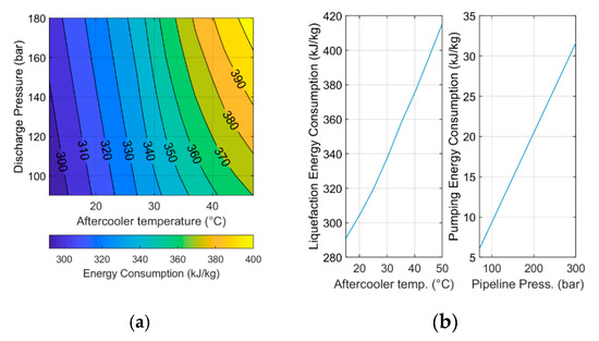
Figure 4. Modeling Basis for the Energy Consumption for Compression, (a) Liquefaction and Pumping Power (b).

2.4. Model Outputs

Based on the input parameters summarized in Table 2, the model generates a set of outputs, which are summarized in Table 4. These outputs can be subsequently used to automatically generate several plots, as summarized in Table 5, by specifying the Plot parameter in Main.

Table 4. Summary of Model Outputs.

Name	Profiles
Elevation	Pipeline element length & element elevation change
Pressure	Pressure profile for 10%, 30% & 50% overpressure
Temperature	Pressure profile for 10%, 30% & 50% overpressure
Name	Performance
Inlet Pressure	Inlet pressure for each pipeline size & overpressure case
WHP	Well head pressure for each overpressure case
Av. Frictional DP	Simple mean of frictional pressure drop component for each case
Av. Velocity	Simple mean of gas velocity pressure drop component for each case
Energy	Summary of energy consumption for each pipeline size & overpressure case.

Table 5. Summary Plots Generated by the Model.

Name	Description
Map	Location map for the pipeline/liquefaction location
Conditions	Plot of temperature vs pressure for all pipe sizes and overpressure cases
Profiles	Pressure and temperature profiles for the smallest line size that operates under 200 bar under all conditions
Energy	Sum of pipeline and liquefaction energy consumption for all pipe sizes and overpressure cases

2.5. Model Validation

The aim of the model validation work was to verify the reliability of the pressure and temperature profile calculations carried out by the model. The method chosen was to use the Aspen HYSYS software package, in order to generate a set of reference data against which the pressure and temperature profile predictions made by the model could be compared. The HYSYS software is a process modeling package that is widely used in the gas processing industry that includes a set of built-in modelling capabilities that are suitable for calculating pipeline pressure and temperature profiles, making it well suited to the validation exercise. The approach taken to the assessment of the validation results was to calculate the absolute value of the pressure and temperature error. The limit for an acceptable validation results was set as an average absolute error of less than 1 °C for the temperature profile and 1 bar for the pressure profile. Further details of the method used in the validation work is presented below.

As the model automatically generates a case-dependent elevation profile that often consists of more than 100 data points it was necessary to construct a simplified profile that could be manually implemented in HYSYS. The simplified profile was created by sampling 19 data points from the Melkøya profile that capture the key features and is stored in a custom case definition called Validation which is saved with the model and can be run using Main. This validation elevation profile is illustrated in Figure 2 and the data points that form the basis are presented in Table 6.

Table 6. Elevation Profile Used in the Validation.

Length (km)	Elevation (m)	Length (km)	Elevation (m)
0.0	0.0	58.7	−310
0.4	−1.2	65.1	−371
0.5	−99.1	76.1	−384
3.1	−127	91.4	−435
18.0	−228	107	−343
21.3	−230	126	−363
25.5	−338	133	−344
39.7	−65.4	145	−341
47.1	−102	149	−321
53.7	−317	152	−322

In the HYSYS model, the Peng Robinson (PR) properties package was used with default options and the mixture in the pipeline was considered to be pure CO₂. In the model, to allow a direct comparison with the HYSYS results, a set of density and heat capacity data was generated from HYSYS that formed the modelling basis for the validation work. This data is stored in the model as a stream called Post_Val.

The inlet pressure calculated by the model was then used to specify the inlet pressure in the HYSYS model so that the results could be directly compared. The results of this validation exercise are stored in full with the model, which is available at UiT Open Research Data [45] and presented below in the Results section.

2.6. Sample Case

As described under earlier headings, the normal basis for the density and heat capacity calculations made by the model is tabulated data from the TREND properties package. Therefore, because the results from the validation study are based on properties data generated using HYSYS, the results are not directly equivalent to the standard model output for the same input parameters. To provide a comparison against the model results for the same case, a sample set of results were generated using the case file called Melkoya, which has the same input parameters as Validation. These results are saved in full with the model available at UiT Open Research Data [45] and can also be generated by running Main with Validation selected as the example case. A summary of these results is presented in the Results.

3. Results

The results provided here are limited to the presentation of a summary of the findings of the validation exercise and the presentation of a single set of results for a Sample Case: the Melkøya CO₂ pipeline using a rough interpretation of the pipeline route from Såtendal et al. [31]. Full results for both of these cases are stored with the model at UiT Open Research Data [45].

3.1. Validation

Figure 5 provides a comparison of the temperature profile generated by the model and HYSYS for the same validation case. Figure 5b shows that the average absolute temperature difference between the two models is less than 1 °C, which indicates that the calculations made by the model are reliable. Figure 6 provides a comparison of the pressure profile generated by the model and HYSYS for the same validation case. Again, the results from the model correspond well with the results from the HYSYS model, with a maximum pressure difference of under 1 bar across the full length of the pipeline.

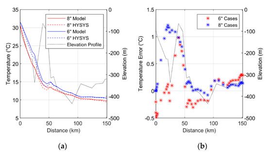
Figure 5. Comparison of Model and HYSYS Results for the Validation Case, (a) shows a Comparison of the Temperature Profile Results for the 10% Overpressure Case; and (b) shows the Absolute Temperature Difference Between the Results.

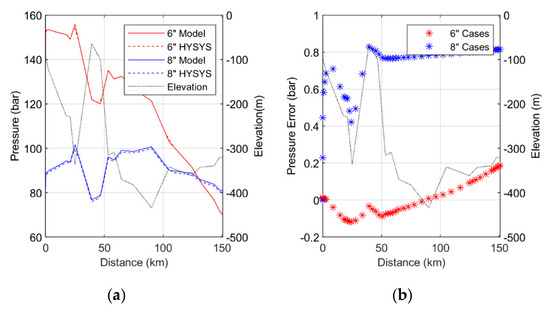
Figure 6. Comparison of Model and HYSYS Results for the Validation Case: (a) Shows a Comparison of the Pressure Profile Results for the 10% Overpressure Case; and (b) Shows the Absolute Pressure Difference Between the Two Sets of Results.

3.2. Sample Case

Figure 7, Figure 8, Figure 9 and Figure 10 present the standard set of model plots as described by Table 4. Figure 9 shows that the smallest pipeline size to ensure operating conditions under 200 bar in all operating cases is 8 inches. Figure 9 also shows that a margin is maintained against the bubble point pressure for all cases across the pipeline length. Figure 10 shows the temperature and pressure profiles for the 10% reservoir overpressure case and illustrates that the minimum pressure condition at the wellhead end only dictates the pipeline inlet pressure for the 6 inch pipeline case due to high pressure drop along the pipeline. In the other cases the minimum pipeline pressure condition (approach to the bubble point pressure) sets the pipeline inlet pressure, which means that some pressure letdown would be required at the wellhead to reach WHP.

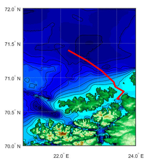
Figure 7. Approximate Melkøya CO₂ Pipeline Route.

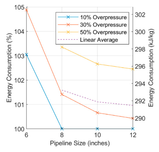
Figure 8. Summary of Energy Consumption for the Melkøya CO₂ Pipeline Example.

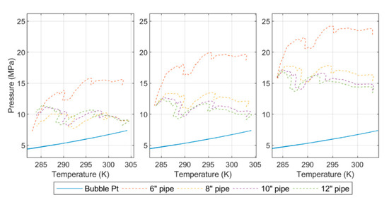
Figure 9. Summary of Pipeline Temperature and Pressure Conditions for the Melkøya CO₂ Pipeline Example. On the left is the 10% reservoir overpressure case, middle 30% and right 50% overpressure.

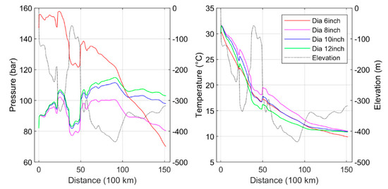
Figure 10. Summary of Pipeline Temperature and Pressure Profiles for the Melkøya CO₂ Pipeline Example for the 10% reservoir overpressure case.

The tabulated data that forms the basis for Figure 5, Figure 6, Figure 9 and Figure 10 is stored with the model and available at UiT Open Research Data [45]. The raw data allows a more detailed comparison of the results obtained using the modelling basis for the validation work (illustrated in Figure 5 and Figure 6) and the results obtained using the standard modelling basis (presented in Figure 9 and Figure 10). For example, the data for the 6 inch line size and the 10% overpressure case shows that the inlet pressure is 144.4 bar in the validation results and 147.0 bar for the default model. A comparison of the 8 inch line outlet pressure for the 10% overpressure case shows 80.9 bar for the validation case and 80.4 bar for the default model basis. Outlet temperatures are also very similar in all cases.

4. Discussions

The scope of this article is the development and validation of a pipeline model; application of the model to compare the performance of different CO₂ pipeline alternatives will form part of future study work. In particular, the model described here is intended for use in the development of larger system models that will include the performance of the capture element of carbon free value chains.

The model presented here is presently only fully developed for the post and pre combustion CO₂ compositions. Data for the oxyfuel stream composition and transportation energy consumption can be calculated by the model, but this is not on a consistent basis with the pre- and post-combustion cases, and therefore, cannot be directly compared with these cases.

The results of the validation work show that the model can reproduce pipeline pressure profiles with good accuracy and that a representative elevation profile can be generated automatically from bathymetry data that captures the key features of a complicated pipeline route such as the one associated with the Melkøya CO₂ pipeline. A comparison of the validation results to the standard modelling basis also shows good agreement.

5. Conclusions

This article has presented the development of a model for CO₂ transportation processes. The model has been validated and tested against an example case, and can be seen to give consistent results.

The results of the validation work show that the pressure and temperature profile have an average absolute error of less than 1 bar, and 1 °C, respectively compared to the selected reference model supporting the aim of the work, which is to provide a consistent and transparent basis for the comparison of different CO₂ transportation scenarios.

The results from the sample case show how the results of the model can be used to provide useful design and performance information for CO₂ pipelines, confirming, for example, that the installed size of 8 inches [31] is the optimum size for the Melkøya pipeline.

The development of comparisons between different transport case will form the scope of future work. The code for the model presented here along with all the data needed for its use and the results presented in this article is available at UiT Open Research Data [45].

References

- Global CCS Institute. Global Status of CCS 2019; Global CCS Institute: Melbourne, Australia, 2019. [Google Scholar]
- IEA. World Energy Outlook 2019; IEA: Paris, France, 2019. [Google Scholar] [CrossRef]
- Peletiri, S.P.; Rahmanian, N.; Mujtaba, I.M. CO2 Pipeline design: A review. Energies 2018, 11, 2184. [Google Scholar] [CrossRef]
- Northern Lights—A European CO2 Transport and Storage Network. Available online: https://northernlightsccs.eu/ (accessed on 5 March 2020).
- Mazzoccoli, M.; Bosio, B.; Arato, E.; Brandani, S. Comparison of equations-of-state with P-p-T experimental data of binary mixtures rich in CO2 under the conditions of pipeline transport. J. Supercrit. Fluids 2014, 95, 474–490. [Google Scholar] [CrossRef]
- Wang, J.; Wang, Z.; Sun, B. Improved equation of CO2 Joule–Thomson coefficient. J. CO2 Util. 2017, 19, 296–307. [Google Scholar] [CrossRef]
- Span, R.E.T.; Herrig, S.; Hielscher, S.; Jäger, A.; Thol, M. TREND. In Thermodynamic Reference and Engineering Data 3.0; Lehrstuhl für Thermodynamik, Ruhr-Universität Bochum: Bochum, Germany, 2016. [Google Scholar]
- Wilhelmsena, Ø.; Skaugena, G.; Jørstadb, O.; Hailong, L. Evaluation of SPUNG# and other Equations of State for use in Carbon Capture and Storage modelling. Energy Procedia 2012, 23, 236–245. [Google Scholar]
- Nazeri, M.; Chapoy, A.; Burgass, R.; Tohidi, B. Viscosity of CO2-rich mixtures from 243 K to 423 K at pressures up to 155 MPa: New experimental viscosity data and modelling. J. Chem. Thermodyn. 2018, 118, 100–114. [Google Scholar] [CrossRef]
- Drescher, M.; Wilhelmsen, Ø.; Aursand, P.; Aursand, E.; de Koeijer, G.; Held, R. Heat Transfer Characteristics of a Pipeline for CO2 Transport with Water as Surrounding Substance. Energy Procedia 2013, 37, 3047–3056. [Google Scholar] [CrossRef][Green Version]
- Lee, W.J.; Yun, R. In-tube convective heat transfer characteristics of CO2 mixtures in a pipeline. Int. J. Heat Mass Transf. 2018, 125, 350–356. [Google Scholar] [CrossRef]
- Wetenhall, B.; Race, J.M.; Aghajani, H.; Barnett, J. The main factors affecting heat transfer along dense phase CO2 pipelines. Int. J. Greenh. Gas Control 2017, 63, 86–94. [Google Scholar] [CrossRef]
- Zhang, W.B.; Shao, D.; Yan, Y.; Liu, S.; Wang, T. Experimental investigations into the transient behaviours of CO2 in a horizontal pipeline during flexible CCS operations. Int. J. Greenh. Gas Control 2018, 79, 193–199. [Google Scholar] [CrossRef]
- Mohammadi, M.; Hourfar, F.; Elkamel, A.; Leonenko, Y. Economic Optimization Design of CO2 Pipeline Transportation with Booster Stations. Ind. Eng. Chem. Res. 2019, 58, 16730–16742. [Google Scholar] [CrossRef]
- McCoy, S.; Rubin, E. An engineering-economic model of pipeline transport of CO2 with application to carbon capture and storage. Int. J. Greenh. Gas Control 2008, 2, 219–229. [Google Scholar] [CrossRef]
- Tian, Q.; Zhao, D.; Li, Z.; Zhu, Q. Robust and stepwise optimization design for CO2 pipeline transportation. Int. J. Greenh. Gas Control 2017, 58, 10–18. [Google Scholar] [CrossRef]
- Deng, H.; Roussanaly, S.; Skaugen, G. Techno-economic analyses of CO2 liquefaction: Impact of product pressure and impurities. Int. J. Refrig. 2019, 103, 301–315. [Google Scholar] [CrossRef]
- Aspelund, A.; Mølnvik, M.J.; De Koeijer, G. Ship Transport of CO2: Technical Solutions and Analysis of Costs, Energy Utilization, Exergy Efficiency and CO2 Emissions. Chem. Eng. Res. Des. 2006, 84, 847–855. [Google Scholar] [CrossRef]
- Knoope, M.M.J.; Ramírez, A.; Faaij, A.P.C. Investing in CO2 transport infrastructure under uncertainty: A comparison between ships and pipelines. Int. J. Greenh. Gas Control 2015, 41, 174–5836. [Google Scholar] [CrossRef]
- Jordal, K.; Aspelund, A. Gas conditioning—The interface between CO2 capture and transport. International Int. J. Greenh. Gas Control 2007, 1, 343–354. [Google Scholar]
- Jackson, S.; Brodal, E. Optimization of the Energy Consumption of a Carbon Capture and Sequestration Related Carbon Dioxide Compression Processes. Energies 2019, 12, 1603. [Google Scholar] [CrossRef]
- Jackson, S.; Brodal, E. Optimization of the CO2 Liquefaction Process-Performance Study with Varying Ambient Temperature. Appl. Sci. 2019, 9, 4467. [Google Scholar] [CrossRef]
- Alabdulkarem, A.; Hwang, Y.H.; Radermacher, R. Development of CO2 liquefaction cycles for CO2 sequestration. Appl. Therm. Eng. 2012, 33, 144–156. [Google Scholar] [CrossRef]
- Seo, Y.; Huh, C.; Lee, S.; Chang, D. Comparison of CO2 liquefaction pressures for ship-based carbon capture and storage (CCS) chain. Int. J. Greenh. Gas Control 2016, 52, 1–12. [Google Scholar] [CrossRef]
- Øi, L.E.; Eldrup, N.H.; Adhikari, U.; Bentsen, M.H.; Badalge, J.C.L.; Yang, S. Simulation and Cost Comparison of CO2 Liquefaction. Energy Proceida 2016, 86, 500–510. [Google Scholar] [CrossRef]
- Jakobsen, J.; Roussanaly, S.; Anantharaman, R. A techno-economic case study of CO2 capture, transport and storage chain from a cement plant in Norway. J. Clean. Prod. 2017, 144, 523–539. [Google Scholar] [CrossRef]
- Jakobsen, J.P.; Roussanaly, S.; Brunsvold, A.; Anantharaman, R. A Tool for Integrated Multi-criteria Assessment of the CCS Value Chain. Energy Procedia 2014, 63, 7290–7297. [Google Scholar] [CrossRef]
- Mallon, W.; Buit, L.; van Wingerden, J.; Lemmens, H.; Eldrup, N.H. Costs of CO2 Transportation Infrastructures. Energy Procedia 2013, 37, 2969–2980. [Google Scholar] [CrossRef]
- The MathWorks. MATLAB; The MathWorks: Natick, MA, USA, 2018. [Google Scholar]
- GEBCO Compilation Group. GEBCO 2019 Grid. 2019. Available online: https://www.gebco.net/data_and_products/gridded_bathymetry_data/gebco_2019/gebco_2019_info.html (accessed on 27 January 2020).
- Såtendal, S.H.; Laug, R.; Oaland, O. Subsea Pipeline Intervention In the Barents Sea. In Proceedings of the Seventeenth International Offshore and Polar Engineering Conference, Lisbon, Portugal, 1 January 2007; p. 7. [Google Scholar]
- Japan Meteorological Agency. Available online: http://ds.data.jma.go.jp/tcc/tcc/products/elnino/cobesst_doc.html (accessed on 1 November 2019).
- Maldal, T.; Tappel, I.M. CO2 underground storage for Snøhvit gas field development. Energy 2004, 29, 1403–1411. [Google Scholar] [CrossRef]
- Shi, J.-Q.; Imrie, C.; Sinayuc, C.; Durucan, S.; Korre, A.; Eiken, O. Snøhvit CO2 Storage Project: Assessment of CO2 Injection Performance Through History Matching of the Injection Well Pressure Over a 32-months Period. Energy Procedia 2013, 37, 3267–3274. [Google Scholar] [CrossRef]
- Vishal, V.; Singh, T.N. Geologic Carbon Sequestration: Understanding Reservoir Behavior; Springer Nature: Cham, Switzerland, 2016. [Google Scholar] [CrossRef]
- Zhang, Z.X.; Wang, G.X.; Massarotto, P.; Rudolph, V. Optimization of pipeline transport for CO2 sequestration. Energy Convers. Manag. 2006, 47, 702–715. [Google Scholar] [CrossRef]
- Roussanaly, S.; Brunsvold, A.L.; Hognes, E.S. Benchmarking of CO2 transport technologies: Part II – Offshore pipeline and shipping to an offshore site. Int. J. Greenh. Gas Control 2014, 28, 283–299. [Google Scholar] [CrossRef]
- Nimtz, M.; Klatt, M.; Wiese, B.; Kühn, M.; Joachim Krautz, H. Modelling of the CO2 process- and transport chain in CCS systems—Examination of transport and storage processes. Geochemistry 2010, 70, 185–192. [Google Scholar] [CrossRef]
- Forbes, S.M.; Verma, P.; Curry, T.E.; Friedmann, S.J.; Wade, S.M. CCS Guidelines: Guidelines for Carbon Dioxide Capture, Transport, and Storage; World Resources Institute: Washington, DC, USA, 2008. [Google Scholar]
- Zigrang, D.; Sylvester, N. Explicit approximations to the solution of Colebrook’s friction factor equation. AIChE J. 1982, 28, 514–515. [Google Scholar] [CrossRef]
- Winning, H.; Coole, T. Explicit Friction Factor Accuracy and Computational Efficiency for Turbulent Flow in Pipes. Int. J. Publ. Assoc. ERCOFTAC 2013, 90, 1–27. [Google Scholar] [CrossRef]
- Langelandsvik, L.I. Modeling of Natural Gas Transport and Friction Factor for Large-Scale Pipelines: Laboratory Experiments and Analysis of Operational Data; Norwegian University of Science and Technology, Faculty of Engineering Science and Technology, Department of Energy and Process Engineering: Trondheim, Norway, 2008. [Google Scholar]
- Jia, W.; Li, C.; Wu, X. Internal Surface Absolute Roughness for Large-Diameter Natural Gas Transmission Pipelines. Oil Gas. Eur. Mag. 2014, 40, 211–213. [Google Scholar]
- Chandel, M.K.; Pratson, L.F.; Williams, E. Potential economies of scale in CO2 transport through use of a trunk pipeline. Energy Convers. Manag. 2010, 51, 2825–2834. [Google Scholar] [CrossRef]
- Jackson, S. Carbon Dioxide Transportation Energy Model; Version 1, UiT; The Arctic University of Norway, Ed.; DataverseNO: Tromsø, Norway, 2020. [Google Scholar] [CrossRef]
© 2020 by the author. Licensee MDPI, Basel, Switzerland. This article is an open access article distributed under the terms and conditions of the Creative Commons Attribution (CC BY) license (http://creativecommons.org/licenses/by/4.0/).