


Abstract
Arctic regions are warming rapidly, elevating extinction risks and accelerating ecosystem change, yet widely used bioclimatic datasets rarely represent polar-specific ecological constraints. Here we present BioClimPolar_2300 v1.0, a raster bioclimatic dataset designed for terrestrial Arctic biodiversity research under climate change. The dataset includes 33 gridded bioclimatic layers at a 10 km spatial resolution, covering seven discrete temporal intervals from 2010 to 2300 AD. In addition to conventional variables used globally, BioClimPolar_2300 incorporates three polar-relevant constraint domains: (1) polar day–night phenomena (PDNs), including degree-day metrics during polar night and polar day; (2) temperature-defined seasonal cycles (TSCs), including seasonal temperature, precipitation, aridity, and season length; (3) hot/cold stresses (HCSs), capturing indices of extreme summer heat and winter cold. Precipitation during snow-melting days (P_melting) is also included due to its relevance for species depending on subnivean habitats. Climate fields were extracted from CMIP6 models and statistically downscaled to 10 km using a change-factor approach under a polar projection. Monthly fields were linearly interpolated to derive daily grids, enabling the computation of variables that require daily inputs. Validation against observations from 30 Arctic weather stations indicates performance suitable for biodiversity applications, and two exemplar range shift case studies (one animal and one plant) illustrate biological relevance and provide practical guidance for data extraction and use. BioClimPolar_2300 fills a key gap in Arctic bioclimatic resources and supports more realistic biodiversity assessments and conservation planning through 2300.
1. Introduction
Arctic regions are undergoing the fastest warming, with a rate nearly double the global mean, and are expected to continue this trend in the future [1,2]. Organisms inhabiting Earth’s coldest environments face a uniquely challenging situation compared to those in other regions, such as a lack of opportunities to shift ranges to cooler areas [3]. This “double forcing” places polar species at extreme extinction risk and threatens ecosystems with a high likelihood of structural and functional collapse [4]. Arctic biodiversity research and nature conservation are among the most urgent topics in global change studies [5,6,7,8]. However, many such studies may be limited by not accounting for unique polar characteristics: specifically, the polar-day and polar-night phenomena (PDNs) [9,10] and temperature-dependent life cycles tied to variable seasonal timing and duration [11].
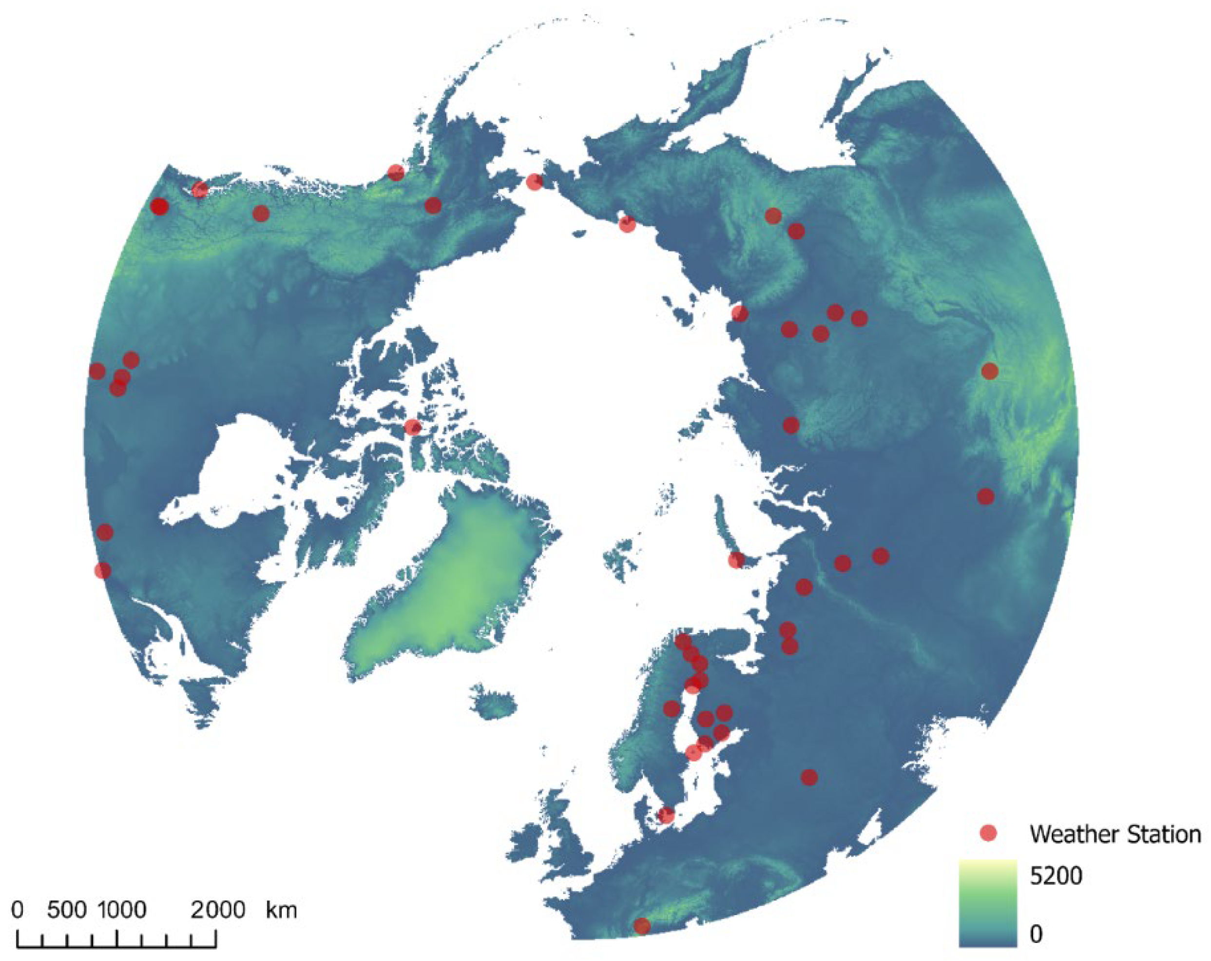
Bioclimatic datasets are essential foundations for numerous ecological studies and conservation plans worldwide. Many local and global datasets are published online and readily available, forming core assets in ecological informatics [12,13]. However, to our knowledge, none are specifically designed for polar regions to address the “double forcing” challenge in high-latitude biodiversity research. Here, we release BioClimPolar_2300 v1.0—a comprehensive bioclimatic dataset covering the entire terrestrial Arctic (Figure 1) at a mesoscale resolution (10 km) extending to 2300 AD.
Figure 1.
Dataset coverage and the weather stations used for validation. Notes: The background map is rendered with elevation data, with red spots indicating weather stations whose observational data were used to validate bioclimatic variable calculations.
The dataset contains 33 bioclimatic variables, with most (25) addressing unique environmental pressures on polar species, and a sub-set (8) applicable to species globally (Table 1). Uniqueness stems from three features incorporating ecological principles: polar-day and -night phenomena (PDNs) [14], temperature-defined seasonal cycles (TSCs) [15], and cold–heat stresses (CHSs) [16]. Four variables relate to PDNs, including cold degree days during polar nights (CDD_PN) and warm degree days during polar days (WDD_PD); 11 variables pertain to TSCs, such as seasonal mean temperature, total precipitation, and aridity (winter aridity excluded for technical reasons), plus season length in days; 8 variables address CHSs, like WDD for hot summer days and CDD for frigid winter days. Total precipitation during snow-melting days (P_melting), though not fitting these categories, is included due to its severe impact on animals relying on subnivean vegetation [17,18].
Table 1.
The 33 bioclimatic variables present in the BioClimPolar_2300 v1.0 dataset.
As CMIP6 climate variables have coarse spatial resolution [21], we applied a statistical downscaling algorithm (change factor method) [19,22] to downscale monthly temperature and precipitation layers to 10 km resolution (polar projection). All bioclimatic variables were calculated from these layers. Most variables require daily calculations (with six exceptions), so we implemented linear interpolation to generate daily raster maps from monthly data—a necessary simplification to achieve computational feasibility on our local systems. Potential inaccuracies from this approach were evaluated using observational data from 30 Arctic weather stations (Figure 1). We further demonstrated the dataset’s utility through exemplar applications predicting range shifts for two species (one animal, one plant). These serve two purposes: demonstrating the biological relevance of the dataset’s unique variables and providing technical guidance for data extraction.
This paper describes (1) the two-step methodology for dataset creation; (2) data access details; (3) validation against observational records and species range shift case studies; (4) recommendations for effective data usage.
2. Methods
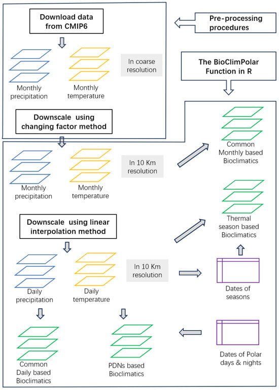
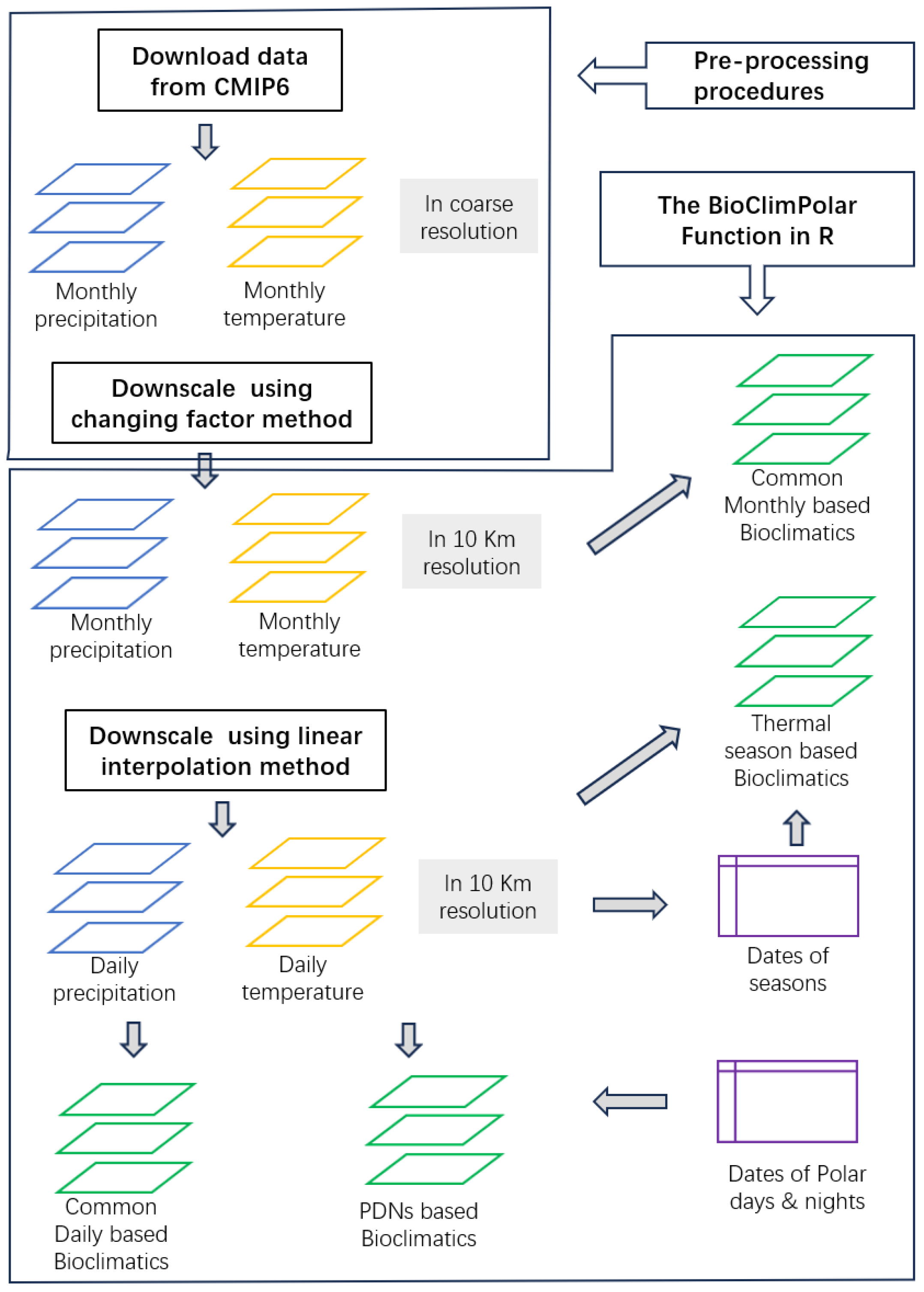
There are two steps in the process (Figure 2) for producing each bundle of layers containing the 33 bioclimatic variables for a specific case (i.e., a given GCM, SSP, and time period). The aggregation of all cases constitutes the BioClimPolar_2300 v1.0 dataset. In this section, we will detail this process, outline the accuracy evaluation procedure, and demonstrate the implementation of the two case studies utilizing this dataset.
Figure 2.
Workflow for producing BioClimPolar_2300 v1.0 dataset. Notes: PNDs denotes polar days and nights; bioclimatics refers to bioclimatic variables; blue indicates precipitation layers, yellow represents temperature layers, green signifies bioclimatic variable layers, and purple designates lookup tables for starting and ending dates of seasons and PNDs.
2.1. Prepossessing Procedures
The preprocessing process includes two steps: one for downloading source data from the CMIP6 website, which provides a helpful search engine (https://esgf-node.llnl.gov/projects/cmip6/, accessed on 25 June 2022). We selected CMIP6 GCMs that provide monthly temperature and precipitation projections through 2300 and cover all three SSP scenarios considered here. Only three models met these requirements and were included in the analysis: ESM2 (https://www.wdc-climate.de/ui/entry?acronym=C6_5243961, accessed on 25 June 2022) [23], IPSL (https://hdl.handle.net/21.14106/f8270bc2151936dffc83a10d69720a61f9de8eaa, accessed on 25 June 2022) [24], and MRIE (https://doi.org/10.1594/WDCC/CMIP5.MXELr8, accessed on 25 June 2022) [25]. All source data were downloaded manually.
In part two, the change factor downscaling process, we first averaged projections into seven 30-year periods centered on the starting period, 2050, 2100, 2150, 2200, 2250, and 2285 (numbers denoting the middle of each period). The starting period varies by GCM or SSP case. Using linear extrapolation, we extended the initial period to 2010 (to align with biological data coverage during 1995–2025) and extended 2285 to 2300 for temporal equidistance. We emphasize that linear extrapolation of monthly precipitation introduces a higher uncertainty than for temperature—users must exercise caution with these data.
The algorithm applied the change factor method to downscale source data (in degree-scale geographic coordinates) to the target resolution/polar projection. Prior to downscaling, layers were reprojected to WGS_1984_Azimuthal_Equidistant (ArcGIS 10.7). As is standard practice [22], this method adds fine-resolution spatial patterns from current climate layers to coarse-resolution future–present climate differences. To reduce stair-step artifacts at coarse-grid boundaries, trends were smoothed to fine scale (typically using R’s focal functions). This statistically downscaled monthly temperature/precipitation from ~100 km to 10 km resolution.
2.2. The BioClimPolar Function in R
There are four pathways to create bioclimatic layers, as shown in Figure 2: (1) Common bioclimatic variables calculated with monthly temperature and precipitation layers. Variables T_mean, T_min, T_max, T_range, P_total, and TP_syn belong to this category and can be easily implemented by R raster stack functions (in R package raster, e.g., stackApply(s_t_m, indices = c (1:12× 0 + 1, fun = mean)). TP_syn is simply the correlation coefficient of monthly temperature and precipitation [19], and thus needs to be self-programmed (Script fun_BioPolar.R).
All the other three categories of variables need to interpolate monthly temperature and precipitation data layers to daily ones (we considered the length of each month to be 30 days for simplicity). Sample codes for temperature are as follows:
|
# --- for temperature ---------------------- for(n in 1:360){ m_start <- as.integer((n+15)/30) m_end <- m_start + 1 x_start <- m_start*30 – 15 x_end <- m_end*30 -15 if(m_start < 1) { y_start <- t_m[[12]] } else { y_start <- t_m[[m_start]] } if(m_end > 12){ y_end <- t_m[[1]] } else { y_end <- t_m[[m_end]] } t_d[[n]] <- y_start + (y_end - y_start) * (n - x_start) / (x_end - x_start) } s_t_d <- stack(t_d) |
Variables derived from these interpolated data layers may differ from observational data; thus, they are evaluated for biases and accuracy later in this paper.
Aridity-related variables required special treatment for computational efficiency. Evapotranspiration (integral to aridity definition via the Thornthwaite method [26]) involves complex temperature-dependent calculations. Direct computation on raster stacks was prohibitively slow, so we developed a lookup table algorithm to accelerate processing. We first precomputed evapotranspiration values across all possible temperatures at 0.5 °C intervals to build the lookup table. Subsequent layer calculations reduced to efficient table lookups, decreasing computation time by two orders of magnitude.
(2) Daily common variables were implemented via R stack functions analogous to monthly variables. These include WDD_10, WDD_20, CDD_10, CDD_20, P_warm, P_cool, P_hot, and P_melting.
(3) Polar days/nights (PDNs) critically influence polar organisms. We defined PDN start/end dates using latitude-dependent lookup tables, then calculated WDDs and CDDs by combining daily temperatures with PDN calendars. Mean temperatures during PDNs (T_PD_mean and T_PN_mean) were derived similarly.
(4) Seasons in our dataset are exclusively defined by daily temperature. Given the inherent smoothing from linear interpolation, daily variability may be underrepresented compared to observational data. We determined seasonal start/end dates per grid cell based on daily temperatures and Julian dates, defining summer as days with T ≥ 10 °C, winter as days with T ≤ −10 °C, spring as days with temperature between −10 °C and 10 °C falling before Julian day 180, and fall as days with temperature between −10 °C and 10 °C occurring after Julian day 180. Using this grid-specific framework, we computed seasonal lengths, temperature/precipitation/aridity metrics, and identified extreme events including hot summer days (≥20 °C) and bitter winter days (≤−20 °C). P_melting (frozen precipitation during snowmelt periods) followed identical computational logic. Collectively, these procedures generated all 14 seasonal and HCS-related variables.
2.3. Accuracy Evaluation Process
Our dataset derives bioclimatic variable layers from GCM projections, making true validation infeasible. However, we assessed algorithm accuracy retrospectively using historical observational data. The change factor spatial downscaling algorithm is well-established and reliable, so we did not re-validate it. Instead, we evaluated accuracy loss specifically from our key simplification: linear interpolation from monthly to daily data layers.
We randomly selected 30 Arctic weather stations with complete daily temperature/precipitation records in 1980, 1990, and 2000. Monthly downscaling mirrored our dataset methodology but applied point-based calculations rather than raster layers. For daily calculations, we replaced interpolated data with observed values. Temperature-defined season boundaries received special treatment: a 7-day moving average smoothed daily temperature fluctuations to stabilize seasonal start or end dates.
Scatter plots visually assessed interpolation effects, with accuracy quantified through regression analysis forcing zero intercept between observed and interpolated values for all non-monthly bioclimatic variables. Accuracy was quantified as the coefficient of determination (R2) between interpolated and observed daily values, while bias was defined as their departure from a 1:1 expectation. Systematic deviation was measured by I_Bias = 1.0 − β, while variance departure was captured by I_Accuracy = R2. Selected plots and full index results are presented in the Technical Validation section.
2.4. Range Shift Modeling for Two Exemplary Species
Dataset Application Example: Two ecologically significant Arctic species were selected to demonstrate the utility of our dataset. Dryas (commonly referenced in paleoclimatology as the “Younger Dryas event” [27] serves as a key climate change indicator. The Arctic hare (Lepus arcticus), recognized for its climate sensitivity [28], was also analyzed. We obtained occurrence records from the Global Biodiversity Information Facility (GBIF; https://www.gbif.org, accessed on 13 August 2022), and then constructed ecological niche models using MaxEnt [29] with default settings for simplicity. Future projections of habitat suitability (logistic output) were generated, and range shift indices were calculated following Kou et al. [20], with the modification of replacing the Dx and Dy indices with the D_pole index to accommodate polar cartography. Positive D_pole values indicate northward range shifts toward the map center (North Pole). Resulting suitability maps and displacement trajectories are presented in the Dataset Utilization and Examples section (Appendix A).
2.5. Other Accessory Procedures
Accessory procedures include sub-procedures of running R scripts to implement the core function BioClimPolar; organizing and storing data in easy-to-understand folder structure and data formats; and miscellaneous tasks to maintain between major processes.
3. Data Records
The data is available at https://doi.org/10.6084/m9.figshare.29400053 (accessed on 15 July 2025). The whole dataset consists of two sub-sets: the pure climate sub-set (Precipitation_Temperature_NetCDF.zip) and the bioclimatic sub-set (BioPolar_NetCDF.zip). These sub-sets possess a similar folder structure. The topmost order folder contains four elements (Current, ESM2, IPSL, and MPIE, the last three are abbreviations of GCM model names); in each GCM, there are three SSPs, namely, SSP126, SSP245, and SSP585; further, each SSP contains seven files, representing seven time periods ranging from 2100 to 2300. Within a file in NetCDF format, there are 33 map layers, each for a bioclimatic variable, or 12 map layers, each corresponding to a monthly value of mean temperature or total precipitation. Summing up the total dataset, there are about 3650 map layers, occupying a 4.88-gigabyte storage space.
4. Technical Validation
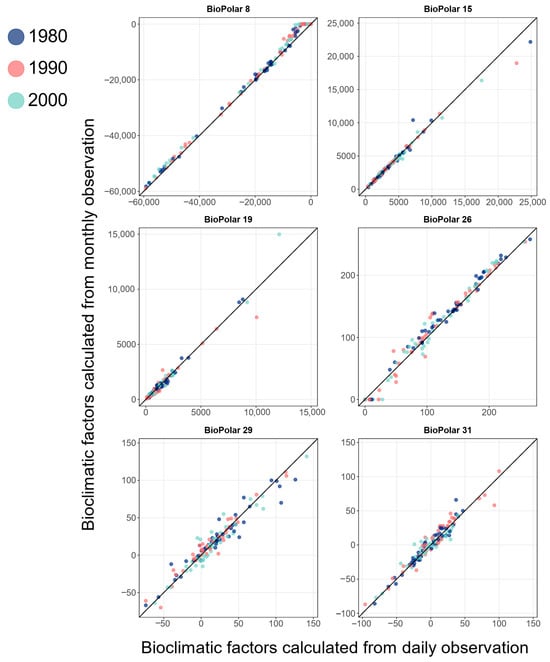
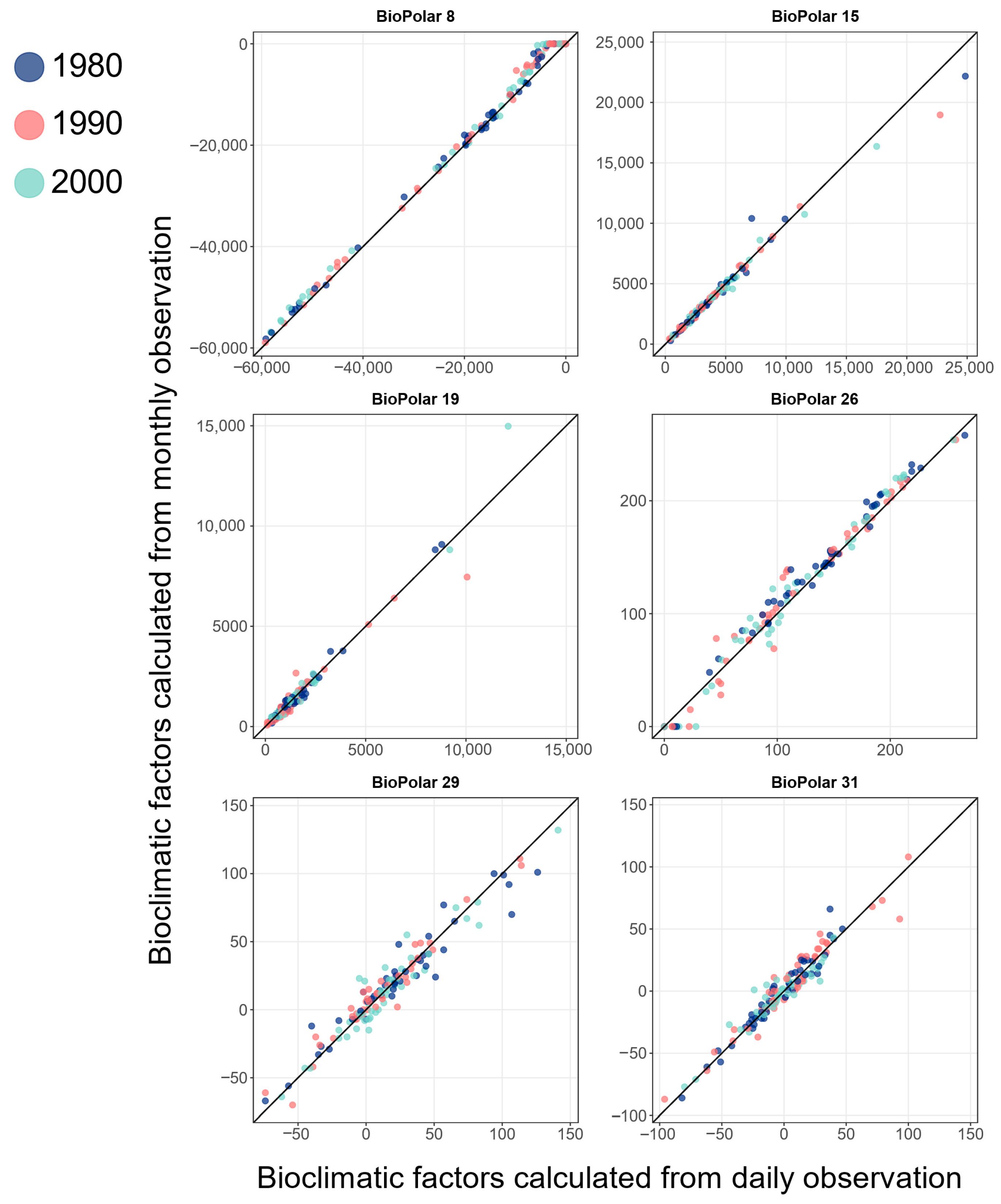
The results demonstrate that our primary simplification algorithm—deriving daily bioclimatic variables by linearly interpolating monthly data—yields generally reliable outputs based on bias/accuracy metrics and scatter plot inspection (Table 2, Figure 3, and Supplementary Figure S1). The median and lower and upper quantiles of bias index for the 29 variables across three time periods (excluding four outliers) are −0.003, 0.024, and 0.053, respectively. The four outlier variables selected based on a bias > 0.20 include Bio_07 (WDD_20), Bio_21 (P_hot), Bio_28 (D_hot), and Bio_32 (A_hot). We note that these exclusively relate to hot-event metrics (temperature thresholds ≥ 20 °C), necessitating cautious interpretation when using such hot-day variables. For improved accuracy in cold/heat stress variables (CHSs), we propose replacing linear interpolation with stochastic weather generators (e.g., Kou et al. [30]). Accuracy indices for non-outlier variables remain high with median = 0.973, lower quantile = 0.990, and upper quantile = 0.995, collectively confirming the algorithm’s reliability, except for CHS-related variables.
Table 2.
Biases and accuracy indices for bioclimatic variables in the validation cases.
Figure 3.
Scatter plots of daily and monthly bioclimatic-variable values based on records from weather stations in Arctic. Notes: Scatter plots compare bioclimatic-variable values derived from daily (x-axis) and monthly (y-axis) algorithms for 30 validation weather stations during 1980, 1990, and 2000 AD. Points aligned on the diagonal line indicate perfect agreement between interpolation methods; deviations quantify calculation inaccuracies.
5. Usage Notes
Users can download the wanted bioclimatic files from the dataset link: https://doi.org/10.6084/m9.figshare.29400053. Each file contains 33 map layers using the NetCDF data format. To extract specific layers from the NetCDF file, the following R code needs to be implemented:
|
# Select layer index to extract (1–33) target_layer < −12 # Example: Layer 12 # Extract coordinates and data layer_data <- ncvar_get(nc, “biopolar”, start = c (1, 1, target_layer), count = c (−1, −1, 1)) |
We provide an exemplar R script (NetCDF_Data_Extraction.R) to assist users in extracting target data. For custom time periods, we strongly recommend interpolating from monthly temperature/precipitation layers before executing the BioClimPolar.R function, rather than interpolating bioclimatic variables directly. This is because approximate linearity only holds for temperature and precipitation, but may not extend reliably to derived bioclimatic variables. Sub-setting regional data is straightforward in R/GIS platforms; however, modifying spatial resolution should similarly begin with monthly temperature/precipitation data layers for consistency with temporal interpolation principles. Therefore, this dataset includes both final bioclimatic variables and foundational monthly climate layers.
6. Code Availability
All code used to generate this dataset—from pre-processed data (downscaled monthly mean temperature and total precipitation) to ancillary scripts for data extraction—is available at https://doi.org/10.6084/m9.figshare.29400053, contained in the file R_scripts.zip. This includes cutting Arctic-specific climate data from global datasets with reprojection; calculating bioclimatic layers from pure climate data; converting said layers from RData to NetCDF format for structured storage; and exemplar scripts for user-specified data layer extraction.
Supplementary Materials
The online version contains supplementary material available at https://doi.org/10.6084/m9.figshare.29400053 (accessed on 15 July 2025) as Figure S1_BioPolarScatterPlot.pdf for Supplementary Figure.
Author Contributions
X.K. produced the overall design and supervised the production of the dataset; Y.S. and S.L. processed all the data and developed R codes for data processing; S.L., B.Y., and Y.Z. ran the code and checked the resultant data layers; Y.S. and X.K. prepared the figures and tables; and X.K. and Y.S. wrote the data paper. All authors have read and agreed to the published version of the manuscript.
Funding
This research was funded by National Key Research and Development Program of China, grant number No. 2020YFA0608504.
Institutional Review Board Statement
Not applicable.
Informed Consent Statement
Not applicable.
Data Availability Statement
The data presented in this study are openly available in [BioClimPolar_2300 Dataset] [https://doi.org/10.6084/m9.figshare.29400053, accessed on 15 July 2025].
Conflicts of Interest
The authors declare no conflicts of interest.
Appendix A. Dataset Utilization Examples
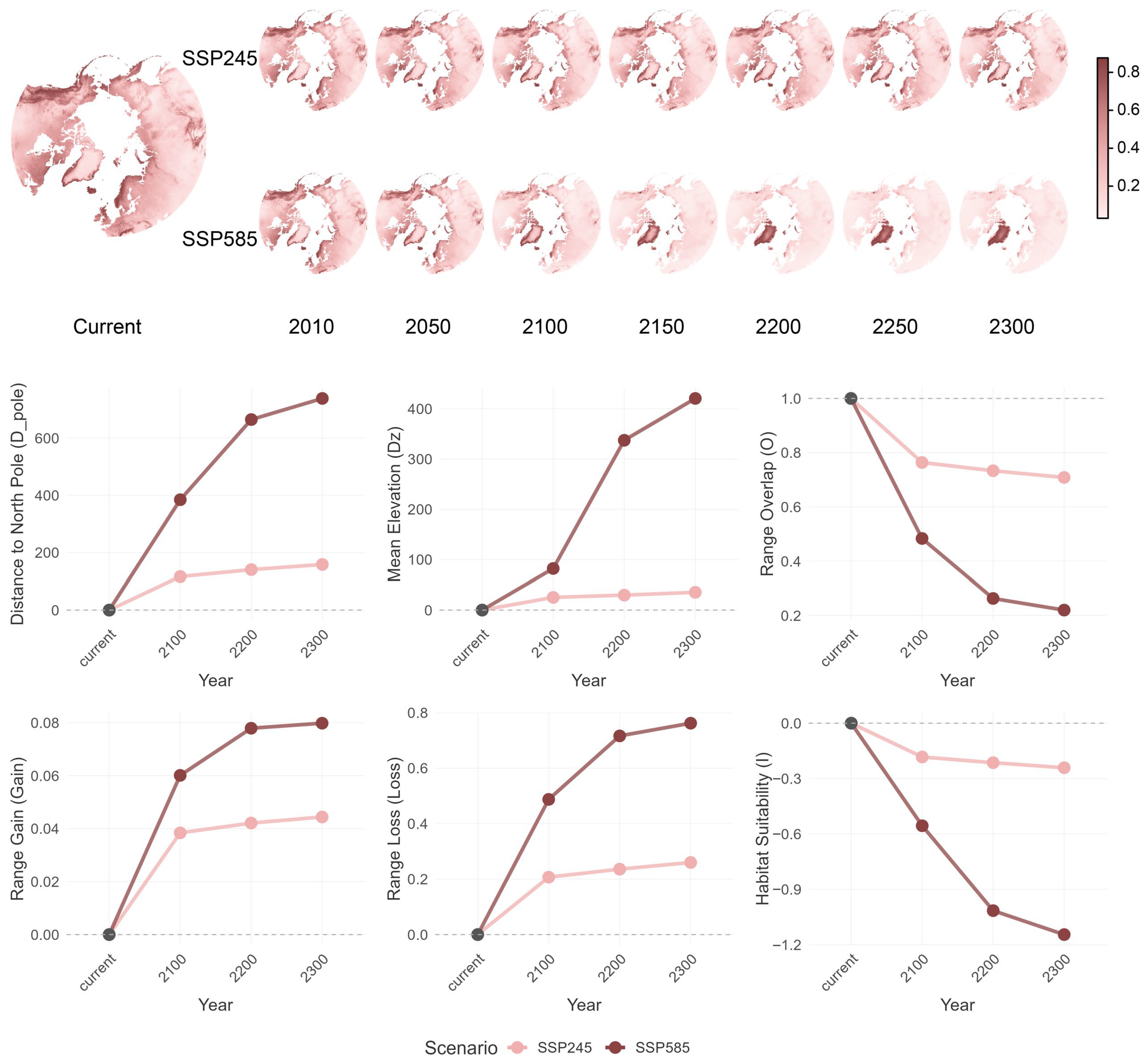
By fitting niche models based on current bioclimatic data layers and occurrence data of Arctic hareand dryasin the MaxEnt platform, we successfully built high-accuracy ecological niches for both focal species (AUC > 0.90). The selected predictors for dryas included Bio_3 (T_max), Bio_9 (CDD_20), Bio_16 (P_cool), and Bio_25 (D_fall); meanwhile, for Arctic hare, they comprised Bio_3 (T_max), Bio_9 (CDD_20), Bio_22 (P_melting), Bio_25 (D_fall), and Bio_33 (TP_syn), demonstrating differences in their ecological requirements. The projected series of species suitability maps and range shift indices conforms to expected Arctic species responses under future climate change (Figure A1 and Figure A2), confirming a primary application scenario for this dataset.
Figure A1.
Range shift maps and shift index curves for Arctic hare (Lepus arcticus). Notes: Upper sections display suitability maps for Arctic hare under current and future climate conditions, derived from bioclimatic variables projected by best-fitted niche model in MaxEnt. Lower sections show time-series curves for range-shifting indices (definitions provided in main text).
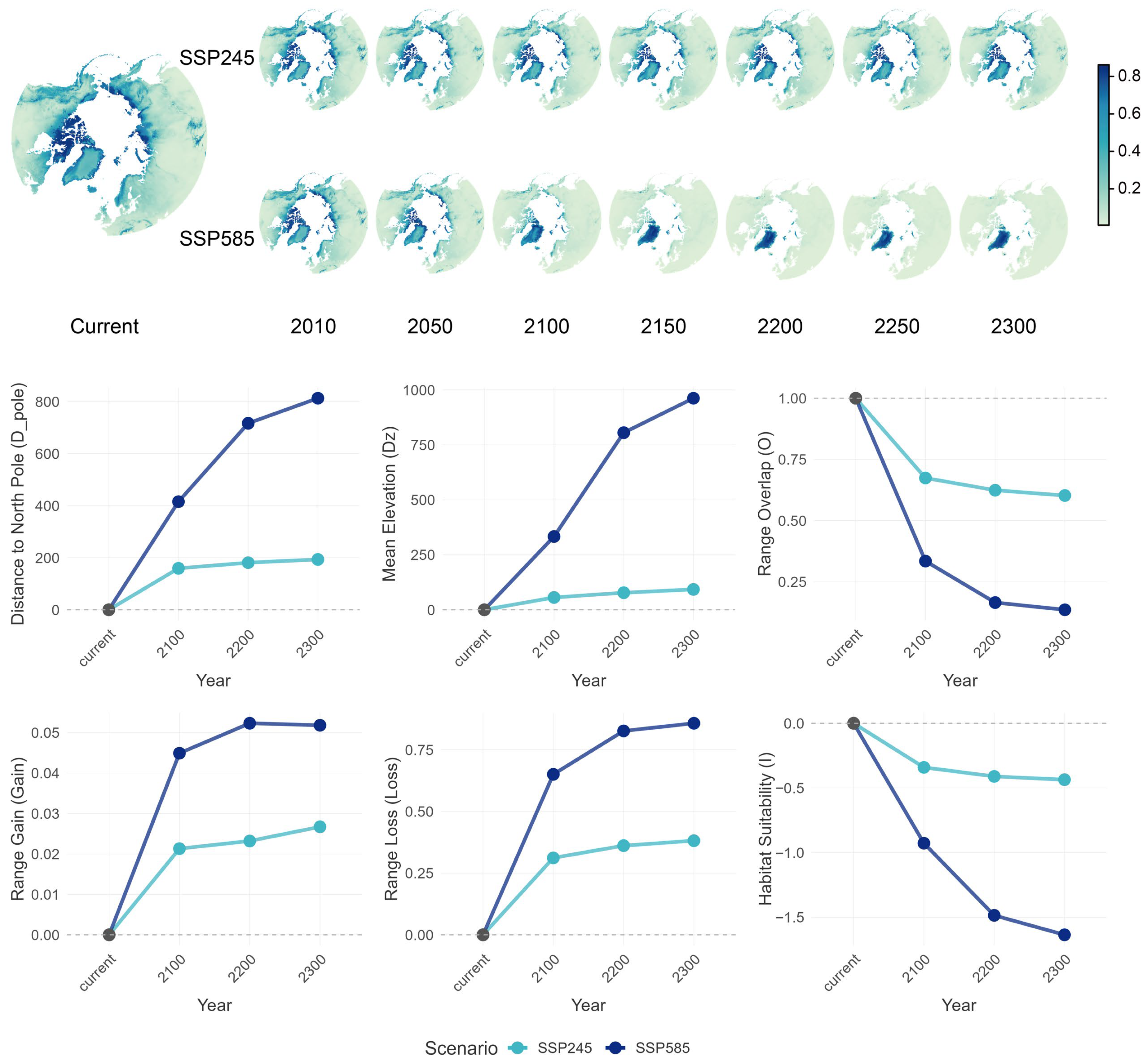
Figure A2.
Range shift maps and shift index curves for Dryas (Dryas octopetala L.). Notes: Upper parts show suitability maps for Dryas under current and future climate conditions based on relevant bioclimatic variables projected from best-fitted niche model in MaxEnt, while lower parts show time-series curves for range-shifting indices (definitions provided in main text).
References
- Chylek, P.; Folland, C.; Klett, J.D.; Wang, M.Y.; Hengartner, N.; Lesins, G.; Dubey, M.K. Annual Mean Arctic Amplification 1970–2020: Observed and Simulated by CMIP6 Climate Models. Geophys. Res. Lett. 2022, 49, e2022GL099371. [Google Scholar] [CrossRef] [Scilit]
- Rantanen, M.; Karpechko, A.Y.; Lipponen, A.; Nordling, K.; Hyvärinen, O.; Ruosteenoja, K.; Vihma, T.; Laaksonen, A. The Arctic has warmed nearly four times faster than the globe since 1979. Commun. Earth Environ. 2022, 3, 168. [Google Scholar] [CrossRef] [Scilit]
- Niskanen, A.K.J.; Niittynen, P.; Aalto, J.; Väre, H.; Luoto, M. Lost at high latitudes: Arctic and endemic plants under threat as climate warms. Divers. Distrib. 2019, 25, 809–821. [Google Scholar] [CrossRef] [Scilit]
- Post, E.; Alley, R.B.; Christensen, T.R.; Macias-Fauria, M.; Forbes, B.C.; Gooseff, M.N.; Iler, A.; Kerby, J.T.; Laidre, K.L.; Mann, M.E.; et al. The polar regions in a 2 °C warmer world. Sci. Adv. 2019, 5, eaaw9883. [Google Scholar] [CrossRef] [Scilit]
- Schaefer, J.A. Increases in graminoids after three decades of change in the High Arctic. Polar Res. 2023, 42, 1–11. [Google Scholar] [CrossRef] [Scilit]
- Myrsky, E.; Mikola, J.; Kaarlejarvi, E.; Olofsson, J.; Sjogersten, S.; Tupek, B.; Mannisto, M.K.; Stark, S. Higher vascular plant abundance associated with decreased ecosystem respiration after 20 years of warming in the forest-tundra ecotone. Funct. Ecol. 2024, 38, 219–232. [Google Scholar] [CrossRef] [Scilit]
- Finne, E.A.; Bjerke, J.W.; Stordal, F.; Tallaksen, L.M. Lichens are more tolerant against winter warming stress than vascular and non-vascular plants: Insights from an alpine field experiment. J. Ecol. 2025, 113, 518–530. [Google Scholar] [CrossRef] [Scilit]
- Quan, Q.; He, N.; Zhang, R.; Wang, J.; Luo, Y.; Ma, F.; Pan, J.; Wang, R.; Liu, C.; Zhang, J.; et al. Plant height as an indicator for alpine carbon sequestration and ecosystem response to warming. Nat. Plants 2024, 10, 890–900. [Google Scholar] [CrossRef] [Scilit]
- Hazlerigg, D.G.; Appenroth, D.; Tomotani, B.M.; West, A.C.; Wood, S.H. Biological timekeeping in polar environments: Lessons from terrestrial vertebrates. J. Exp. Biol. 2023, 226, jeb246308. [Google Scholar] [CrossRef] [Scilit]
- Blix, A.S. Adaptations to polar life in mammals and birds. J. Exp. Biol. 2016, 219, 1093–1105. [Google Scholar] [CrossRef] [Scilit] [PubMed]
- Ruthrauff, D.R.; Patil, V.P.; Hupp, J.W.; Ward, D.H. Life-history attributes of Arctic-breeding birds drive uneven responses to environmental variability across different phases of the reproductive cycle. Ecol. Evol. 2021, 11, 18514–18530. [Google Scholar] [CrossRef] [Scilit] [PubMed]
- Noce, S.; Caporaso, L.; Santini, M. A new global dataset of bioclimatic indicators. Sci. Data 2020, 7, 398. [Google Scholar] [CrossRef] [Scilit]
- Fick, S.E.; Hijmans, R.J. WorldClim 2: New 1-km spatial resolution climate surfaces for global land areas. Int. J. Climatol. 2017, 37, 4302–4315. [Google Scholar] [CrossRef] [Scilit]
- Horodynski, E.M. The Building for the Yearly Cycle: A Bioclimatic and Biophilic Approach Exemplified on the Circumpolar North. Master’s Thesis, Technischen Universität Wien, Wien, Austria, 2021. [Google Scholar]
- Mellard, J.P.; Audoye, P.; Loreau, M. Seasonal patterns in species diversity across biomes. Ecology 2019, 100, e02627. [Google Scholar] [CrossRef] [Scilit]
- Zaninović, K. Limits of warm and cold bioclimatic stress in different climatic regions. Theor. Appl. Climatol. 1992, 45, 65–70. [Google Scholar] [CrossRef] [Scilit]
- Kankaanpää, T.; Skov, K.; Abrego, N.; Lund, M.; Schmidt, N.M.; Roslin, T. Spatiotemporal snowmelt patterns within a high Arctic landscape, with implications for flora and fauna. Arct. Antarct. Alp. Res. 2018, 50, e1415624. [Google Scholar] [CrossRef] [Scilit]
- Heggberget, T.M.; Gaare, E.; Ball, J.P. Reindeer (Rangifer tarandus) and climate change: Importance of winter forage. Rangifer 2002, 22, 13–31. [Google Scholar] [CrossRef] [Scilit]
- Kou, X.; Li, Q.; Liu, S. High-resolution bioclimatic dataset derived from future climate projections for plant species distribution modeling. Ecol. Inform. 2011, 6, 196–204. [Google Scholar]
- Kou, X.; Li, Q.; Beierkuhnlein, C.; Zhao, Y.; Liu, S. A new tool for exploring climate change induced range shifts of conifer species in China. PLoS ONE 2014, 9, e98643. [Google Scholar] [CrossRef] [Scilit]
- Tebaldi, C.; Debeire, K.; Eyring, V.; Fischer, E.; Fyfe, J.; Friedlingstein, P.; Knutti, R.; Lowe, J.; O’Neill, B.; Sanderson, B. Climate model projections from the scenario model intercomparison project (ScenarioMIP) of CMIP6. Earth Syst. Dyn. 2021, 12, 253–293. [Google Scholar] [CrossRef] [Scilit]
- Diaz-Nieto, J.; Wilby, R.L. A comparison of statistical downscaling and climate change factor methods: Impacts on low flows in the River Thames, United Kingdom. Clim. Change 2005, 69, 245–268. [Google Scholar] [CrossRef] [Scilit]
- Yukimoto, S.; Koshiro, T.; Kawai, H.; Oshima, N.; Yoshida, K.; Urakawa, S.; Tsujino, H.; Deushi, M.; Tanaka, T.; Hosaka, M. MRI MRI-ESM2.0 Model Output Prepared for CMIP6 CMIP; Earth System Grid Federation (ESGF): Livermore, CA, USA, 2019. [Google Scholar]
- Boucher, O.; Denvil, S.; Levavasseur, G.; Cozic, A.; Caubel, A.; Foujols, M.-A.; Meurdesoif, Y.; Gastineau, G. IPSL IPSL-CM6A-LR Model Output Prepared for CMIP6 DAMIP; World Data Center for Climate (WDCC): Hamburg, Germany, 2018. [Google Scholar]
- Giorgetta, M.; Jungclaus, J.; Reick, C.; Legutke, S.; Brovkin, V.; Crueger, T.; Esch, M.; Fieg, K.; Glushak, K.; Gayler, V. CMIP5 Simulations of the Max Planck Institute for Meteorology (MPI-M) Based on the MPI-ESM-LR Model: The rcp85 Experiment, Served by ESGF; World Data Center for Climate (WDCC): Hamburg, Germany, 2011. [Google Scholar]
- Pereira, A.R.; Pruitt, W.O. Adaptation of the Thornthwaite scheme for estimating daily reference evapotranspiration. Agric. Water Manag. 2004, 66, 251–257. [Google Scholar] [CrossRef] [Scilit]
- Joosten, J. Between diluvium and deluge: The origin of the Younger Dryas concept. Neth. J. Geosci. 1995, 237–240. [Google Scholar]
- Gray, D.R. Behavioural adaptations to Arctic winter: Shelter seeking by Arctic hare (Lepus arcticus). Arctic 1993, 340–353. [Google Scholar] [CrossRef] [Scilit]
- Elith, J.; Phillips, S.J.; Hastie, T.; Dudik, M.; Chee, Y.E.; Yates, C.J. A statistical explanation of MaxEnt for ecologists. Divers. Distrib. 2011, 17, 43–57. [Google Scholar] [CrossRef] [Scilit]
- Kou, X.; Ge, J.; Wang, Y.; Zhang, C. Validation of the weather generator CLIGEN with daily precipitation data from the Loess Plateau, China. J. Hydrol. 2007, 347, 347–357. [Google Scholar] [CrossRef] [Scilit]

Disclaimer/Publisher’s Note: The statements, opinions and data contained in all publications are solely those of the individual author(s) and contributor(s) and not of MDPI and/or the editor(s). MDPI and/or the editor(s) disclaim responsibility for any injury to people or property resulting from any ideas, methods, instructions or products referred to in the content. |
© 2026 by the authors. Licensee MDPI, Basel, Switzerland. This article is an open access article distributed under the terms and conditions of the Creative Commons Attribution (CC BY) license.