Study on Date–Jimbo–Kashiwara–Miwa Equation with Conformable Derivative Dependent on Time Parameter to Find the Exact Dynamic Wave Solutions

Abstract

In this article, we construct the exact dynamical wave solutions to the Date–Jimbo–Kashiwara–Miwa equation with conformable derivative by using an efficient and well-established approach, namely: the two-variable $\left(G’/G, 1/G\right)$-expansion method. The solutions of the Date–Jimbo–Kashiwara–Miwa equation with conformable derivative play a vital role in many scientific occurrences. The regular dynamical wave solutions of the abovementioned equation imply three different fundamental functions, which are the trigonometric function, the hyperbolic function, and the rational function. These solutions are classified graphically into three categories, such as singular periodic solitary, kink soliton, and anti-kink soliton wave solutions. Furthermore, the effect of the fractional parameter on these solutions is discussed through 2D plots.

1. Introduction

Many phenomena are represented by nonlinear partial differential equations known as quasi linear or nonlinear evolution equations. Almost all of the occurrences in our natural world, especially in the science and engineering sectors, can be simulated by this complicated mathematical equation, which are space- and time-related, nonlinear evolution equations (NLEEs). To explain the natural incidents occurred in many scientific fields—such as the field of engineering, solid-state physics, plasma physics, applied physics, applied mathematics, plasma waves, fluid dynamics, quantum physics, electrodynamics, magneto hydrodynamics and turbulence, biology, fiber optics, chemistry, chemical physics, astrophysics, general theory of relativity, cosmology, medical science, and so on [1,2,3,4,5,6,7,8,9,10,11,12,13,14,15,16,17,18,19,20,21,22,23,24,25,26,27,28,29,30,31,32,33,34,35,36,37,38,39,40,41,42,43,44,45,46,47,48]—we need to look for the exact solutions of the NLEEs. Many researchers have built up various types of methods to obtain the exact solutions for the NLEEs, including the following: the homogeneous balance method [1,2], the first integral method [3,4], the Jacobi elliptic function expansion method [5,6], the exponential function method [7,8], the tanh–function method [9,10], the auxiliary ordinary differential equation method [11], the homotopy analysis method [12], the tanh–coth method [13], the sine–Gordon expansion method [14], the ($G^{\prime }$/$G^2$)-expansion method [15], the unified method [16], the variational iteration method [17], the extended direct algebraic method [18], the exp($-\varphi \left(\xi \right)$)-expansion method [19,20], Lie group method [21], the Hirota’s bilinear method [22,23], the generalized Kudryshov method [24,25,26], the Backlund transform method [27], the Cole–Hopf transformation method [28], the Riccati equation method [29], the $\left(G^{\prime }/G\right)$-expansion method [30,31], the new generalized $(G’/G)$expansion method [32], the modified $(G’/G)$-expansion method [33], and so on.

Inc et al. [34] proposed the two-variable $\left(G’/G, 1/G\right)$-expansion method to solve the Kaup–Kupershmidt equation, while Miah et al. [35] used this technique to investigate different exact traveling wave solutions of some NLEEs. In [36,37,38], many researchers have used this method to solve many other NLEEs. In this paper, we investigate the conformable Date–Jimbo–Kashiwara–Miwa (CDJKM) equation, and we solve it by using the two-variable $\left(G’/G, 1/G\right)$-expansion method. The CDJKM equation moved to (2 + 1)-dimensional Date–Jimbo–Kashiwara–Miwa equation when the fractional derivative $\theta =1$. Many researchers investigated the (2 + 1)-dimensional Date–Jimbo–Kashiwara–Miwa equation [39,40,41,42], but no one used our desired method to solve the CDIKM equation. For the first time, Guo and Lin [44] introduced the CDJKM equation and Kumar et al. [45] successfully investigated the solutions for this equation via the sine–Gordon expansion and the improved Bernoulli sub equation methods. In [45], only one real solution is presented, and the rest of the solutions are complex. Therefore, our purpose here is to present new real wave solutions for the CDJKM equation by using the two-variable $\left(G’/G, 1/G\right)$-expansion method and explain the dynamical behavior of the obtained solutions.

The CDJKM equation has the following form [43,44]:

$$u_{xxxxy}+4u_{xxy}{u}_x+2u_{xxx}{u}_y+6u_{xy}{u}_{xx}-\alpha u_{yyy}-2\beta \frac{\partial }{\partial x}\left(\frac{\partial }{\partial x}\left(\frac{{\partial }^{\theta }u}{\partial t^{\theta }}\right)\right)=0$$

(1)

where $u=u\left(x,y,t\right)$, $\beta$ is a constant, and $0<\theta \le 1$.

The rest of the paper is organized as follows: in Section 2, the construction of the two-variable $\left(G’/G, 1/G\right)$-expansion method is stated. In Section 3, the solutions of the CDJMK equation are investigated via the $\left(G’/G, 1/G\right)$-expansion method. In Section 4, the graphical representation of the obtained solutions is introduced through some 3D and 2D plots. Finally, the conclusion is presented in Section 5.

2. Explanation of the Two-Variable (G’/G, 1/G)-Expansion Method

In this part, we shortly discuss the two-variable $\left(G’/G, 1/G\right)$-expansion method.

Consider an auxiliary non-homogeneous second order linear ordinary differential equation (ODE), as follows:

$$\frac{d^{2}G}{d{\eta }^2}+\lambda G=\mu$$

(2)

where $\lambda$ and $\mu$ are constants. Assume the following two relations:

$$L=\frac{G’\left(\eta \right)}{G\left(\eta \right)}, H=\frac{1}{G\left(\eta \right)}$$

(3)

By using Equations (2) and (3), we obtain two new relations, as follows:

$$L^{\prime }=-L^2+\mu H-\lambda , H^{\prime }=-LH.$$

(4)

Equation (2) has three types of general solutions, depending on $\lambda$, which can be classified as follows:

ConditionI. For $\lambda >0,$ Equation (2) has a general solution in the following form:

$$G\left(\eta \right)=A \sin \left(\sqrt{\lambda }\eta \right)+B \cos \left(\sqrt{\lambda }\eta \right)+\frac{\mu }{\lambda }$$

(5)

Consequently, we have the following:

$$H^2=\frac{\lambda \left(L^2-2\mu H+\lambda \right)}{{\lambda }^2{\rho }_1-{\mu }^2}$$

(6)

where ${\rho }_1=A^2+B^2$ and $A, B$ are two arbitrary constants.

ConditionII. For $\lambda <0,$ Equation (2) has a general solution in the following:

$$G\left(\eta \right)=A \sin \mathrm{h}\left(\sqrt{-\lambda }\eta \right)+B \cos \mathrm{h}\left(\sqrt{-\lambda }\eta \right)+\frac{\mu }{\lambda }$$

(7)

Therefore, we have the following:

$$H^2=\frac{-\lambda \left(L^2-2\mu H+\lambda \right)}{{\lambda }^2{\rho }_2+{\mu }^2}$$

(8)

where ${\rho }_2=A^2-B^2$.

ConditionIII. For $\lambda =0,$ Equation (2) has a general solution in the following form:

$$G\left(\eta \right)=\frac{\mu }{2}{\eta }^2+A\eta +B$$

(9)

Thus, we have the following:

$$H^2=\frac{\left(L^2-2\mu H\right)}{A^2-2\mu B}$$

(10)

Now, consider the following nonlinear partial differential equation:

$$R\left(u, u_x, u_t, u_y, u_t, u_{xx}, u_{xy}, u_{yy}, u_{tt}, u_t^{\theta }, u^2, . . .\right)=0$$

(11)

where $R$ is a polynomial in $u\left(x, y, t\right)$ and it is partial derivatives.

Action 1. Convert the function $u$ of the three independents variables $x, y, \mathrm{and} t$ into a function of single parameter by the following conventional wave transformation rule, as follows:

$$u\left(x, y, t\right)=u\left(\eta \right), \eta =lx+py-c\frac{t^{\theta }}{\theta }$$

(12)

where $l$ (coefficient of spatial variable $x$), $p$ (coefficient of spatial variable $y$), and $c$ (velocity of wave) are nonzero arbitrary constants. Using Equation (12) in Equation (11), we obtain the following converted nonlinear ordinary equation:

$$Q\left(u, u^{\prime }, u^{″}, u^2, \dots \right)=0$$

(13)

where $Q$ is a polynomial in its arguments.

Action 2. Assume the solution of Equation (13), which can be written in terms of $L\left(\eta \right)$ and $H\left(\eta \right)$, has the following form:

$$u\left(\eta \right)={{\displaystyle \sum }}_{j=0}^M{a}_j{L}^j+{{\displaystyle \sum }}_{j=1}^M{b}_j{L}^{j-1}H$$

(14)

where $a_j \left(j=0, 1, 2, \dots , M\right)$, $b_j \left(j=1, 2, \dots , M\right),$ $c, \lambda , \mathrm{and} \mu$ are constants to be determined later. By applying the homogeneous balance rule between the highest order derivative and the highest nonlinear term, the number $M$ can be evaluated.

Action 3. Insert the value of $M$in Equation (14) and substitute Equation (14) into Equation (13) through Equations (4) and (6), we convert the left side of Equation (13) in terms of $L \mathrm{and} H,$ where the degree of $L$ is taken from zero to any positive integer number but the degree of H cannot be greater than one.

Action 4. Comparing the like powers of the polynomial from both sides then we have a system of algebraic equations in $a_{j,} b_{j, } c, \lambda , \mu , A, \mathrm{and} B$. By using any computation software, like Mathematica, we can solve the obtained algebraic system. By inserting these values into Equation (14), we obtain the solution of Equation (13), and after setting the value of $\eta =lx+py-c\frac{t^{\theta }}{\theta }$ in Equation (11), we reach the desirable traveling wave solution of Equation (11). For more details about the proposed method, see [35,36,37,38].

3. Regular Traveling Wave Solutions of the CDJKM Equation

In this section, the two-variable $\left(G’/G, 1/G\right)$-expansion method is applied to solve the CDJKM equation. By using the wave transformation rule given by Equation (11), we convert Equation (1) into a nonlinear ODE, as follows:

$$l^{4}p{u}^{‴}+3l^{3}p{\left(u^{\prime }\right)}^2-\left(\alpha p^3-2l^{2}c\beta \right)u^{\prime }=0$$

(15)

Now after setting $u^{\prime }=U$, we obtain the following:

$$l^{4}p{U}^{″}+3l^{3}p{U}^2-\left(\alpha p^3-2l^{2}c\beta \right)U=0$$

(16)

where the prime indicates the derivative with respect to $\eta$.

By applying the homogeneous balance rule between $U^{″}$ and $U^2$ in Equation (16), we obtain $M=2$. Thus, the general solution takes the following form:

$$U\left(\eta \right)=a_0+a_{1}L\left(\eta \right)+a_2{L}^2\left(\eta \right)+b_{1}H\left(\eta \right)+b_{2}L\left(\eta \right)H\left(\eta \right)$$

(17)

where $a_j \left(j=0, 1, 2, \dots , M\right)$ and $b_{j }\left(j=1, 2, \dots , M\right)$ are constants and the new functions $L\left(\eta \right)$ and $H\left(\eta \right)$ are defined in Equation (4).

Now, Equation (16) have three types of solutions which have the following cases:

ConditionI. For $\lambda >0.$Differentiate Equation (17) two times, and by using Equations (4) and (6), Equation (16) is converted in terms of $L\left(\eta \right) and H\left(\eta \right)$. By comparing the coefficients of the required polynomial from both sides, we obtain a group of algebraic equations in $a_0, a_1,a_2, b_1, b_2, \lambda and c$. After solving this algebraic system, we obtain two different sets of solutions.

Set 1:

$$a_0=-l\lambda , a_1=0, a_2=-l, b_1=l\mu , b_2=\pm \frac{l\sqrt{{\lambda }^2{\rho }_1-{\mu }^2}}{\sqrt{\lambda }} \mathrm{and} \mathrm{c}=\frac{p\left(p^2\alpha +l^4\lambda \right)}{2l^2\beta }$$

(18)

Set 2:

$$a_0=-\frac{2l\lambda }{3}, a_1=0, a_2=-l, b_1=l\mu , b_2=\pm \frac{l\sqrt{{\lambda }^2{\rho }_1-{\mu }^2}}{\sqrt{\lambda }} \mathrm{and} c=\frac{p\left(p^2\alpha -l^4\lambda \right)}{2l^2\beta }$$

(19)

Now, after putting these values into Equation (17), we obtain the solutions of Equation (16). Firstly, inserting the values from Equation (18) into Equation (17), we find the following:

$$\begin{gathered} U\left(\eta \right)=-l\lambda -l\lambda {\left[\frac{A\cos \left(\sqrt{\lambda }\eta \right)-B\sin \left(\sqrt{\lambda }\eta \right)}{A\cos \left(\sqrt{\lambda }\eta \right)+B\sin \left(\sqrt{\lambda }\eta \right)+\frac{\mu }{\lambda }}\right]}^2+\frac{l\mu }{\left[A\cos \left(\sqrt{\lambda }\eta \right)+B\sin \left(\sqrt{\lambda }\eta \right)+\frac{\mu }{\lambda }\right]} \\ \pm l\sqrt{{\lambda }^2{\rho }_1-{\mu }^2}\frac{\left[A\cos \left(\sqrt{\lambda }\eta \right)-B\sin \left(\sqrt{\lambda }\eta \right)\right]}{{\left[A\cos \left(\sqrt{\lambda }\eta \right)+B\sin \left(\sqrt{\lambda }\eta \right)+\frac{\mu }{\lambda }\right]}^2} \end{gathered}$$

(20)

Equation (20) is one of the solutions of Equation (16). After integrating Equation (20), we attain a generalized trigonometric function solution of Equation (15) and if we substitute $\eta =lx+py-\frac{p\left(p^2\alpha +l^4\lambda \right)}{2l^2\beta }\frac{t^{\theta }}{\theta }$ in the obtained integrand equation, we obtain the desired solution of Equation (1).

For a specific solution, we choose $A=0 \mathrm{and} \mu =0 \mathrm{but} B\ne 0$ in Equation (20), as follows:

$$U\left(\eta \right)=-l\lambda {\sec }^2(\sqrt{\lambda }\eta )\pm l\lambda \tan \left(\sqrt{\lambda }\eta \right) \sec \left(\sqrt{\lambda }\eta \right).$$

(21)

Integrating the above equation, we obtain the solution Equation (15), as follows:

$$u\left(x,y,t\right)=-l\sqrt{\lambda }\tan (\sqrt{\lambda }\eta )\pm l\sqrt{\lambda } \sec \left(\sqrt{\lambda }\eta \right)$$

(22)

where $\eta =lx+py-\frac{p\left(p^2\alpha +l^4\lambda \right)}{2l^2\beta }\frac{t^{\theta }}{\theta }$and both $l$ and $\beta$ are nonzero.

Again, by taking $B=0 \mathrm{but} A\ne 0$ in Equation (20), as follows:

$$U\left(\eta \right)=-\frac{A l {\lambda }^2\cos \left(\sqrt{\lambda }\eta \right) \left(\mu -R_1+2A\lambda \cos \left(\sqrt{\lambda }\eta \right) \right)}{{\left(\mu +A\lambda \cos \left(\sqrt{\lambda }\eta \right)\right)}^2}$$

(23)

where $R_1=\sqrt{{\lambda }^2{\rho }_1-{\mu }^2}$. Integrating the above equation, we obtain another solution of Equation (15), as follows:

$$u\left(x,y,t\right)=-A l\sqrt{\lambda }\left[\frac{2\eta \sqrt{\lambda } }{A}+\frac{2\left(-2{\mu }^3+A^2{\lambda }^2 \left(R_1+3\mu \right)\right){\tanh }^{-1}\left(\frac{\left(-A\lambda +\mu \right)\tan \left(\sqrt{\lambda }\eta /2\right)}{R_2}\right) }{A{R}_2^3}+\frac{R_2\lambda \mu \left(R_1+\mu \right)\sin \left(\sqrt{\lambda }\eta \right)}{R_2^3\left(\mu +A\lambda \cos \left(\sqrt{\lambda }\eta \right)\right) }\right]$$

(24)

where $R_2=\sqrt{A^2{\lambda }^2-{\mu }^2}$, $\eta =lx+py-\frac{p\left(p^2\alpha +l^4\lambda \right)}{2l^2\beta }\frac{t^{\theta }}{\theta }$and both $l$ and $\beta$ are nonzero.

Similarly, inserting the values from Equation (19) into Equation (17), we find the following:

$$\begin{gathered} U\left(\eta \right)=-\frac{2l\lambda }{3}-l\lambda {\left[\frac{A\cos \left(\sqrt{\lambda }\eta \right)-B\sin \left(\sqrt{\lambda }\eta \right)}{A\cos \left(\sqrt{\lambda }\eta \right)+B\sin \left(\sqrt{\lambda }\eta \right)+\frac{\mu }{\lambda }}\right]}^2+\frac{l\mu }{\left[A\cos \left(\sqrt{\lambda }\eta \right)+B\sin \left(\sqrt{\lambda }\eta \right)+\frac{\mu }{\lambda }\right]} \\ \pm l\sqrt{{\lambda }^2{\rho }_1-{\mu }^2}\frac{\left[A\cos \left(\sqrt{\lambda }\eta \right)-B\sin \left(\sqrt{\lambda }\eta \right)\right]}{{\left[A\cos \left(\sqrt{\lambda }\eta \right)+B\sin \left(\sqrt{\lambda }\eta \right)+\frac{\mu }{\lambda }\right]}^2} \end{gathered}$$

(25)

Equation (25) is one of the solutions of Equation (16). By integrating Equation (25), we obtain another generalized trigonometric function solution of Equation (15) and if we put $\eta =lx+py-\frac{p\left(p^2\alpha -l^4\lambda \right)}{2l^2\beta }\frac{t^{\theta }}{\theta }$ into the attained integrand equation, we reach the desired solution of Equation (1).

For a particular solution, we choose $A=0 \mathrm{and} \mu =0 \mathrm{but} B\ne 0$ in Equation (25), as follows:

$$U\left(\eta \right)=-\frac{2l\lambda }{3}-l\lambda {\tan }^2(\sqrt{\lambda }\eta )\pm l\lambda \tan \left(\sqrt{\lambda }\eta \right)\sec \left(\sqrt{\lambda }\eta \right).$$

(26)

By integrating Equation (26), we obtain a special solution of Equation (15), as follows:

$$u\left(x,y,t\right)=\frac{l\lambda }{3}\eta -l\sqrt{\lambda }\tan (\sqrt{\lambda }\eta )\pm l\sqrt{\lambda }\sec \left(\sqrt{\lambda }\eta \right),$$

(27)

where $\eta =lx+py-\frac{p\left(p^2\alpha -l^4\lambda \right)}{2l^2\beta }\frac{t^{\theta }}{\theta }$and both $l$ and $\beta$ are nonzero.

Again, for $B=0 \mathrm{and} \mu =0 \mathrm{but} A\ne 0,$ we have the following:

$$U\left(\eta \right)=-\frac{2l\lambda }{3}-l\lambda {\cot }^2(\sqrt{\lambda }\eta )\pm l\lambda \cot \left(\sqrt{\lambda }\eta \right)\cos \mathrm{ec}\left(\sqrt{\lambda }\eta \right).$$

(28)

By integrating Equation (28), we obtain a particular solution of Equation (15), as the following:

$$u\left(x,y,t\right)=\frac{l\lambda }{3}\eta +l\sqrt{\lambda }\cot (\sqrt{\lambda }\eta )\pm l\sqrt{\lambda }\cos \mathrm{ec}\left(\sqrt{\lambda }\eta \right),$$

(29)

where $\eta =lx+py-\frac{p\left(p^2\alpha -l^4\lambda \right)}{2l^2\beta }\frac{t^{\theta }}{\theta }$and both $l$ and $\beta$ are nonzero.

Condition II. For $\lambda <0$.

By the same way, in Condition I, we have also two sets of values of those arbitrary constants, as follows:

Set 1:

$$a_0=-l\lambda , a_1=0, a_2=-l, b_1=l\mu , b_2=\pm \frac{l\sqrt{{\mu }^2+{\lambda }^2{\rho }_2}}{\sqrt{-\lambda }}, c=\frac{p\left(p^2\alpha +l^4\lambda \right)}{2l^2\beta }$$

(30)

Set 2:

$$a_0=-\frac{2l\lambda }{3}, a_1=0, a_2=-l, b_1=l\mu , b_2=\pm \frac{l\sqrt{{\mu }^2+{\lambda }^2{\rho }_2}}{\sqrt{-\lambda }}, c=\frac{p\left(p^2\alpha -l^4\lambda \right)}{2l^2\beta }$$

(31)

After inserting these values into Equation (17), we obtain the solutions of Equation (16). At first, inserting the values from Equation (30) into Equation (17), we find the following:

$$\begin{gathered} U\left(\eta \right)=-l\lambda +l\lambda {\left[\frac{A\cos \mathrm{h}\left(\sqrt{-\lambda }\eta \right)+B\sin \mathrm{h}\left(\sqrt{-\lambda }\eta \right)}{B\cos \mathrm{h}\left(\sqrt{-\lambda }\eta \right)+A\sin \mathrm{h}\left(\sqrt{-\lambda }\eta \right)+\frac{\mu }{\lambda }}\right]}^2 \\ +\frac{l\mu }{\left[B\cos \mathrm{h}\left(\sqrt{-\lambda }\eta \right)+A\sin \mathrm{h}\left(\sqrt{-\lambda }\eta \right)+\frac{\mu }{\lambda }\right]}\pm \\ l\sqrt{{\mu }^2+{\lambda }^2{\rho }_2}\frac{\left[Acosh\left(\sqrt{-\lambda }\eta \right)+Bsinh\left(\sqrt{-\lambda }\eta \right)\right]}{{\left[B \cos \mathrm{h}\left(\sqrt{-\lambda }\eta \right)+A \sin \mathrm{h}\left(\sqrt{-\lambda }\eta \right)+\frac{\mu }{\lambda }\right]}^2} \end{gathered}$$

(32)

Equation (32) is hyperbolic type solution of Equation (16). By integrating Equation (32), we attain a generalized hyperbolic function solution of Equation (15) and if we substitute $\eta =lx+py-\frac{p\left(p^2\alpha +l^4\lambda \right)}{2l^2\beta }\frac{t^{\theta }}{\theta }$ in the obtained integrand equation, we obtain the desired solution of Equation (1).

Now, for a specific solution, we choose $A=0 \mathrm{but} B\ne 0$ in Equation (32), as follows:

$$U\left(\eta \right)=-\frac{B l {\lambda }^2\left(B\lambda +\mu \cos \mathrm{h}\left(\sqrt{-\lambda }\eta \right)-R_{3}s\mathrm{inh}\left(\sqrt{-\lambda }\eta \right) \right)}{{\left(\mu +B\lambda \cos \mathrm{h}\left(\sqrt{-\lambda }\eta \right)\right)}^2}$$

(33)

where $R_3=\sqrt{{\lambda }^2{\rho }_2+{\mu }^2}.$ By integrating Equation (33), we obtain a particular solution of Equation (15), as the following:

$$u\left(x,y,t\right)=\frac{ l\sqrt{-\lambda }\left(R_3+B\lambda s\mathrm{inh}\left(\sqrt{-\lambda }\eta \right) \right)}{\left(\mu +B\lambda \cos \mathrm{h}\left(\sqrt{-\lambda }\eta \right)\right)}$$

(34)

where $\eta =lx+py-\frac{p\left(p^2\alpha +l^4\lambda \right)}{2l^2\beta }\frac{t^{\theta }}{\theta }$and both $l$ and $\beta$ are nonzero.

Again, inserting the values from Equation (31) into Equation (17), we find the following:

$$U\left(\eta \right)=-\frac{2l\lambda }{3}+l\lambda {\left[\frac{A\cos \mathrm{h}\left(\sqrt{-\lambda }\eta \right)+B\sin \mathrm{h}\left(\sqrt{-\lambda }\eta \right)}{A\sin \mathrm{h}\left(\sqrt{-\lambda }\eta \right)+B\cos \mathrm{h}\left(\sqrt{-\lambda }\eta \right)+\frac{\mu }{\lambda }}\right]}^2+\frac{l\mu }{\left[A\sin \mathrm{h}\left(\sqrt{-\lambda }\eta \right)+B\cos \mathrm{h}\left(\sqrt{-\lambda }\eta \right)+\frac{\mu }{\lambda }\right]}\pm l\sqrt{{\mu }^2+{\lambda }^2{\rho }_2}\frac{\left[A\cos \mathrm{h}\left(\sqrt{-\lambda }\eta \right)+B\sin \mathrm{h}\left(\sqrt{-\lambda }\eta \right)\right]}{{\left[A\sin \mathrm{h}\left(\sqrt{-\lambda }\eta \right)+B\cos \mathrm{h}\left(\sqrt{-\lambda }\eta \right)+\frac{\mu }{\lambda }\right]}^2}$$

(35)

Equation (35) is another hyperbolic-type solution of Equation (16). After integrating Equation (35), we have a generalized hyperbolic function solution of Equation (15) and if we substitute $\eta =lx+py-\frac{p\left(p^2\alpha -l^4\lambda \right)}{2l^2\beta }\frac{t^{\theta }}{\theta }$ in the obtained integrand equation, we reach the desired solution of Equation (1).

Now, we take $A=0, \mu =0 \mathrm{but} B\ne 0$ in Equation (35), as follows:

$$U\left(\eta \right)=\frac{ \lambda l{\sec \mathrm{h}}^2\left(\sqrt{-\lambda }\eta \right) \left(-B+\sqrt{{\rho }_2}s\mathrm{inh}\left(\sqrt{-\lambda }\eta \right) \right)}{B}$$

(36)

where $\lambda <0.$ By integrating Equation (36), we obtain a particular solution of Equation (15), as the following:

$$u\left(x,y,t\right)=\frac{ \sqrt{-\lambda } l\sec \mathrm{h}\left(\sqrt{-\lambda }\eta \right) \left(\sqrt{{\rho }_2}+Bs\mathrm{inh}\left(\sqrt{-\lambda }\eta \right) \right)}{B}$$

(37)

where $\eta =lx+py-\frac{p\left(p^2\alpha +l^4\lambda \right)}{2l^2\beta }\frac{t^{\theta }}{\theta }$and both $l$ and $\beta$ are nonzero.

Condition III. For $\lambda =0.$By the same process in the previous two cases, we have only one set of values of the given arbitrary constants, as follows:

Set 1:

$$a_0=0, a_1=0, a_2=-l, b_1=l\mu , b_2=\pm l\sqrt{A^2-2\mu B}, c=\frac{p^3\alpha }{2l^2\beta }$$

(38)

Putting these values from into Equation (17), we find the solution of Equation (16), as follows:

$$U\left(\eta \right)=-l{\left(\frac{\mu \eta +A}{\frac{\mu }{2}{\eta }^2+A\eta +B}\right)}^2+\frac{l\mu }{\frac{\mu }{2}{\eta }^2+A\eta +B}\pm l\sqrt{A^2-2\mu B}\frac{\left(\mu \eta +A\right)}{{\left(\frac{\mu }{2}{\eta }^2+A\eta +B\right)}^2}$$

(39)

Equation (39) is the rational-type solution of Equation (16). After integrating Equation (39), we attain a generalized rational function solution of Equation (15) and if we substitute $\eta =lx+py-\frac{p^3\alpha }{2l^2\beta }\frac{t^{\theta }}{\theta }$ in the obtained integrand equation, we obtain the desired solution of Equation (1).

Setting $B=0, \mu =0$ but $A \ne 0$ in Equation (39), as follows:

$$U\left(\eta \right)=-\frac{2l}{ {\eta }^2}$$

(40)

By integrating Equation (40), we obtain a particular solution of Equation (15), as the following:

$$u\left(x,y,t\right)=\frac{2l}{\eta }$$

(41)

where $\eta =lx+py-\frac{p^3\alpha }{2l^2\beta }\frac{t^{\theta }}{\theta }$and both $l$ and $\beta$ are nonzero.

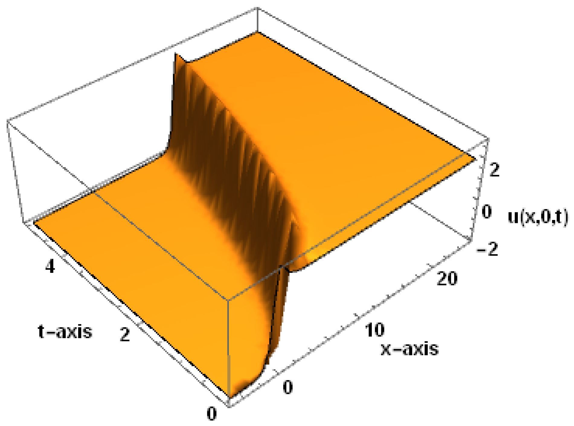
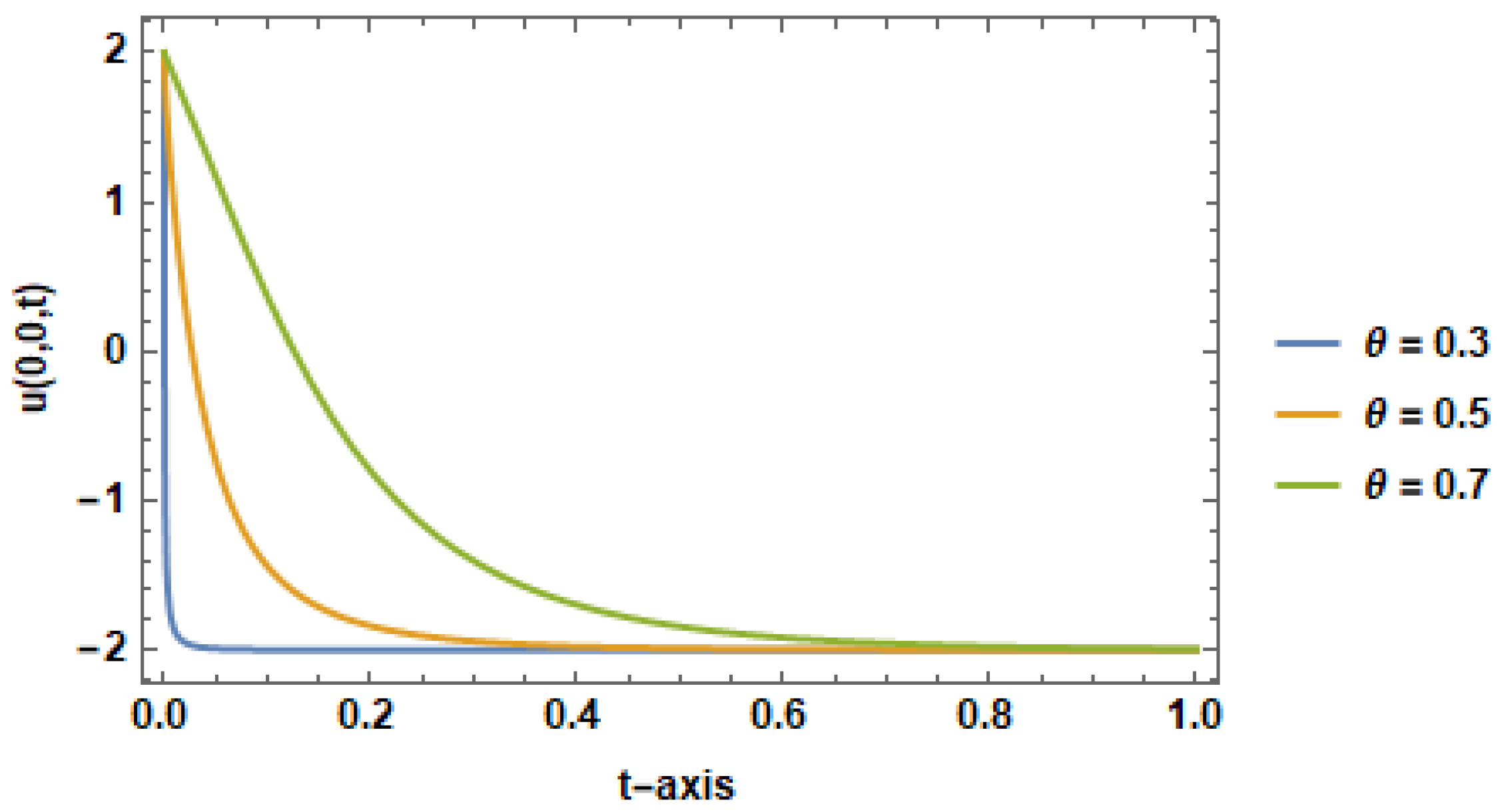
4. Figures and Discussion

In this section, the physical illustration of the obtained wave solutions of the CDJMK equation is investigated. The solutions are trigonometric, hyperbolic, and rational solutions, which are sketched in 3D and 2D shapes in Figure 1, Figure 2, Figure 3, Figure 4, Figure 5 and Figure 6. The 3D figures indicate the singular periodic solitary, kink soliton, and anti-kink soliton wave solutions. In Figure 1, solution (24) indicates the singular periodic solitary wave solution for the values $\alpha =2$, $l=1$, $p=1$, $\lambda =4,\mu =5,$ $\beta =1$, $A=1, \theta =0.5,$ and ${\rho }_1=2$. The corresponding 2D shape for the solution (24) is depicted in Figure 2 for different values of the fractional parameter $\theta$. In Figure 3, the solution given by (34) implies the kink soliton wave solution for the values $\alpha =2$, $l=1$, $p=1$, $\lambda =-4,\mu =4,$ $\beta =1$, $B=-1, \theta =0.5,$ and ${\rho }_2=1$. The corresponding 2D shape for the solution (34) is depicted in Figure 4 for different values of the fractional parameter $\theta .$ In Figure 5, the solution (37) implies an anti-kink shape soliton wave solution when $\alpha =2$, $l=1$, $p=1$, $\lambda =-4,\mu =0,$ $\beta =1$, $B=-1, \theta =0.5,$ and ${\rho }_2=1$. The corresponding 2D shape for the solution (34) is depicted in Figure 6 for different values of the fractional parameter $\theta .$ It is clear that in all 2D figures, for small fractional time derivative, wave progresses are changed significantly. Additionally, we notice that the amplitude of the solution given in Figure 1 and Figure 2 is very high in the medium through which the wave is propagated, thus this singular periodic wave is a schock wave.

5. Conclusions

In this paper, the two-variable$\left(G’/G, 1/G\right)$-expansion method has been applied as a powerful tool to obtain a variety of exact solutions for the CDJMK equation. The obtained solutions are trigonometric, hyperbolic, and rational function solutions. These solutions have different wave structures, such as singular periodic solitary, kink soliton, and anti-kink soliton wave solutions, which have many applications in the modern science and engineering sectors. It is worth mentioning that we attained nine new exact traveling wave solutions by using this eminent method, which are very effective for further investigation into the CDJMK equation. The attained solutions in this article may have momentous effects on future understandings of the natural world, and it is proven that the two-variable $\left(G’/G, 1/G\right)$-expansion method is an adequate, useful, compatible, and important mathematical instrument for obtaining solutions to other NLEEs. The process of the $\left(G’/G, 1/G\right)$-expansion method is easier, more expansive, and more effective than any other well-known methods. In future works, the two-variable $\left(G’/G,1/G\right)$-expansion method can be implemented into different fractional nonlinear systems with variable coefficients; thus, the new exact solutions and their dynamical behaviors can be acquired.

References

1. Wang, M.L.; Zhou, Y.B.; Li, Z.B. Application of a homogeneous balance method to exact solutions of nonlinear equations in mathematical physics. Phys. Lett. A 1996, 216, 67–75. [Google Scholar] [CrossRef]
2. Fan, E.; Zhang, H. A note on the homogeneous balance method. Phys. Lett. A 1998, 246, 403–406. [Google Scholar] [CrossRef]
3. Mahak, N.; Akram, G. Exact solitary wave solutions of the (1+1)-dimensional Fokas-Lenells equation. Optik 2020, 208, 1–9. [Google Scholar] [CrossRef]
4. Rezazadeh, H.; Manafian, J.; Khodadad, F.S.; Nazari, F. Traveling wave solutions for density dependent conformable fractional diffusion-reaction equation by the first integral method and the improved tan ( φ ξ / 2 )-expansion method. Opt. Quantum Electron. 2018, 50, 1–15. [Google Scholar]
5. Lü, D. Jacobi elliptic function solutions for two variant Boussinesq equations. Chaos Soliton Fractals 2005, 24, 1373–1385. [Google Scholar] [CrossRef]
6. Chen, Y.; Wang, Q. Extended Jacobi elliptic function rational expansion method and abundant families of Jacobi elliptic function solutions to (1+1)-dimensional dispersive long wave equation. Chaos Soliton Fractals 2005, 24, 745–757. [Google Scholar] [CrossRef]
7. Bekir, A. Application of the exp-function method for nonlinear differential-difference equations. Appl. Math. Comput. 2010, 215, 4049–4053. [Google Scholar] [CrossRef]
8. He, J.-H.; Wu, X.-H. Exp-function method for nonlinear wave equations. Chaos, Solitons Fractals 2006, 30, 700–708. [Google Scholar] [CrossRef]
9. Fan, E. Extended tanh-function method and its applications to nonlinear equations. Phys. Lett. A 2000, 277, 212–218. [Google Scholar] [CrossRef]
10. Parkes, E.; Duffy, B. An automated tanh-function method for finding solitary wave solutions to non-linear evolution equations. Comput. Phys. Commun. 1996, 98, 288–300. [Google Scholar] [CrossRef]
11. Zhang, Z.Y. Exact traveling wave solutions of the perturbed Klein-Gordon equation with quadratic nonlinearity in (1+1)-dimension. Part I: Without local inductance and dissipation effect. Turk. J. Phys. 2013, 37, 259–267. [Google Scholar] [CrossRef]
12. Domairry, G.; Mohsenzadeh, A.; Famouri, M. The application of homotopy analysis method to solve nonlinear differential equation governing Jeffery–Hamel flow. Commun. Nonlinear Sci. Numer. Simul. 2009, 14, 85–95. [Google Scholar] [CrossRef]
13. Kumar, A.; Pankaj, R.D. Tanh–coth scheme for traveling wave solutions for Nonlinear Wave Interaction model. J. Egypt. Math. Soc. 2015, 23, 282–285. [Google Scholar] [CrossRef] [Green Version]
14. Ali, K.K.; Osman, M.; Abdel-Aty, M. New optical solitary wave solutions of Fokas-Lenells equation in optical fiber via Sine-Gordon expansion method. Alex. Eng. J. 2020, 59, 1191–1196. [Google Scholar] [CrossRef]
15. Ali, M.N.; Osman, M.S.; Husnine, S.M. On the analytical solutions of conformable time-fractional extended Zakharov-Kuznetsov equation through ( G / G 2 )-expansion method and the modified Kudryashov method. SeMA J. 2019, 76, 15–25. [Google Scholar]
16. Abdel-Gawad, H.I.; Osman, M. On shallow water waves in a medium with time-dependent dispersion and nonlinearity coefficients. J. Adv. Res. 2014, 6, 593–599. [Google Scholar] [CrossRef] [PubMed] [Green Version]
17. Abdel-Gawad, H.I.; Osman, M.S. On the Variational Approach for Analyzing the Stability of Solutions of Evolution Equations. Kyungpook Math. J. 2013, 53, 661–680. [Google Scholar] [CrossRef] [Green Version]
18. Gao, W.; Rezazadeh, H.; Pinar, Z.; Baskonus, H.M.; Sarwar, S.; Yel, G. Novel explicit solutions for the nonlinear Zoomeron equation by using newly extended direct algebraic technique. Opt. Quantum Electron. 2020, 52, 1–13. [Google Scholar] [CrossRef]
19. Raza, N.; Aslam, M.R.; Rezazadeh, H. Analytical study of resonant optical solitons with variable coefficients in Kerr and non-Kerr law media. Opt. Quantum Electron. 2019, 51, 59. [Google Scholar] [CrossRef]
20. Raza, N.; Afzal, U.; Butt, A.R.; Rezazadeh, H. Optical solitons in nematic liquid crystals with Kerr and parabolic law nonlinearities. Opt. Quantum Electron. 2019, 51, 107. [Google Scholar] [CrossRef]
21. Jafari, H.; Kadkhoda, N.; Baleanu, D. Fractional Lie group method of the time-fractional Boussinesq equation. Nonlinear Dyn. 2015, 81, 1569–1574. [Google Scholar] [CrossRef]
22. Liu, J.-G.; Eslami, M.; Rezazadeh, H.; Mirzazadeh, M. Rational solutions and lump solutions to a non-isospectral and generalized variable-coefficient Kadomtsev–Petviashvili equation. Nonlinear Dyn. 2018, 95, 1027–1033. [Google Scholar] [CrossRef]
23. Wazwaz, A.M. The Hirota’s bilinear method and the tanh-coth method for multiple-soliton solutions of the Sawada-Kotera-Kadomstsev-Petviashvili equation. Appl. Math. Comput. 2008, 200, 160–166. [Google Scholar]
24. Ali, K.K.; Osman, M.S.; Baskonus, H.M.; Elazabb, N.S.; Ilhan, E. Analytical and numerical study of the HIV-1 infection of CD4 + T-cells conformable fractional mathematical model that causes acquired immunodeficiency syndrome with the effect of antiviral drug therapy. Math. Methods Appl. Sci. 2020. [Google Scholar] [CrossRef]
25. Habib, M.A.; Ali, H.M.S.; Miah, M.M.; Akbar, M.A. The generalized Kudryshov method for new closed form traveling wave solutions to some NLEEs. AIMS Math. 2019, 4, 896–909. [Google Scholar] [CrossRef]
26. Rahman, M.M.; Habib, M.A.; Ali, H.M.S.; Miah, M.M. The generalized Kudryshov method: A renewed mechanism for performing exact solitary wave solutions of some NLEEs. J. Mech. Cont. Math Sci. 2019, 14, 323–339. [Google Scholar]
27. Jianming, L.; Jie, D.; Wenjun, Y. Bäcklund Transformation and New Exact Solutions of the Sharma-Tasso-Olver Equation. Abstr. Appl. Anal. 2011, 2011, 1–8. [Google Scholar] [CrossRef] [Green Version]
28. Sales, A.H.; Gomez, C.A. Application of the Cole-Hopf transformation for finding exact solutions to several forms of the seventh-order KDV equation. Math. Probl. Eng. 2010. [Google Scholar] [CrossRef]
29. Malwe, B.H.; Betchewe, G.; Doka, S.Y.; Kofane, C.T. Travelling wave solutions and soliton solutions for the nonlinear transmission line using the generalized Riccati equation mapping method. Nonlinear Dyn. 2015, 84, 171–177. [Google Scholar] [CrossRef]
30. Wang, M.L.; Li, X.Z.; Zang, J.L. The G’⁄G-expansion method and traveling wave solutions of nonlinear evolution equation in mathematical physics. Phys. Lett. A 2008, 372, 417–423. [Google Scholar] [CrossRef]
31. Hossain, D.; Alam, K.; Akbar, M.A. Abundant wave solutions of the Boussinesq equation and the (2+1)-dimensional extended shallow water wave equation. Ocean Eng. 2018, 165, 69–76. [Google Scholar] [CrossRef]
32. Rani, A.; Hssan, Q.; Ayub, K.; Ahmad, J.; Zulfiqar, A. Soliton solutions of Nonlinear Evolution Equations by Basic (G’/G)-Expansion Method. Math. Model. Eng. Probl. 2020, 7, 242–250. [Google Scholar] [CrossRef]
33. Naher, H.; Abdullah, F.A. The improved G / G -expansion method to the (2+1)-dimensional breaking soliton equation. J. Comput. Anal. Appl. 2014, 16, 220–235. [Google Scholar]
34. Naher, H.; Abdullah, F.A. New generalized and improved G / G -expansion method for nonlinear evolution equations in mathematical physics. Egypt. Math. Soc. 2014, 22, 390–395. [Google Scholar]
35. Inc, M.; Miah, M.; Akher, C.; Ali, S.; Rezazadeh, H.; Akinlar, M.A.; Chu, Y.-M. New exact solutions for the Kaup-Kupershmidt equation. AIMS Math. 2020, 5, 6726–6738. [Google Scholar] [CrossRef]
36. Li, L.X.; Li, E.Q.; Wang, M.L. The ( G / G , 1/ G )-expansion method and its application to traveling wave solutions of the Zakharov equations. Appl. Math.-A J. Chin. Univ. 2010, 25, 454–462. [Google Scholar]
37. Zayed, E.M.E.; Alurrfi, K.A.E. The ( G / G , 1/ G )-expansion method and its applications to two nonlinear Schr o ¨ dinger equations describing the propagation of femtosecond pulses in nonlinear optical fibers. Optik 2016, 127, 1581–1589. [Google Scholar]
38. Chowdhury, M.A.; Miah, M.M.; Ali, H.S.; Chu, Y.-M.; Osman, M. An investigation to the nonlinear (2 + 1)-dimensional soliton equation for discovering explicit and periodic wave solutions. Results Phys. 2021, 23, 104013. [Google Scholar] [CrossRef]
39. Yuan, Y.Q.; Tian, B.; Sun, W.R.; Chai, J.; Liu, L. Wronskian and Grammian solutions for a (2+1)-dimensional Date-Jimbo-Kashiwara-Miwa equation. Comput. Math. Appl. 2017, 74, 873–879. [Google Scholar] [CrossRef]
40. Singh, M.; Gupta, R.K. On Painleve’ analysis, symmetry group and conservation laws of Date-Jimbo-Kashiwara-Miwa equation. Int. J. Appl. Comput. Math. 2018, 4, 88. [Google Scholar] [CrossRef]
41. Wang, S.N.; Hu, J. Grammian solutions for a (2+1)-dimensional integrable coupled modified Date-Jimbo-Kashiwara-Miwa equation. Mod. Phys. Lett. B 2019, 33, 1950119. [Google Scholar] [CrossRef]
42. Ali, K.K.; Mehanna, M.S.; Wazwaz, A.-M. Analytical and numerical treatment to the (2+1)-dimensional Date-Jimbo-Kashiwara-Miwa equation. Nonlinear Eng. 2021, 10, 187–200. [Google Scholar] [CrossRef]
43. Ismael, H.F.; Seadawy, A.; Bulut, H. Rational solutions, and the interaction solutions to the (2 + 1)-dimensional time-dependent Date–Jimbo–Kashiwara–Miwa equation. Int. J. Comput. Math. 2021, 98, 2369–2377. [Google Scholar] [CrossRef]
44. Guo, F.; Lin, J. Interaction solutions between lump and stripe soliton to the (2+1)-dimensional Date-Jimbo-Kashiwara-Miwa equation. Nonlinear Dyn. 2019, 96, 1233–1274. [Google Scholar] [CrossRef]
45. Kumar, A.; Ilhan, E.; Ciancio, A.; Yel, G.; Baskonus, H.M. Extractions of some new travelling wave solutions to the conformable Date-Jimbo-Kashiwara-Miwa equation. AIMS Math. 2021, 6, 4238–4264. [Google Scholar] [CrossRef]
46. Kumar, S.; Kumar, R.; Osman, M.S.; Samet, B. A wavelet based numerical scheme for fractional order SEIR epidemic of measles by using Genocchi polynomials. Numer. Methods Partial. Differ. Equ. 2020, 37, 1250–1268. [Google Scholar] [CrossRef]
47. Osman, M.S.; Abdel-Gawad, H.I. Multi-wave solutions of the (2+1)-dimensional Nizhnik-Novikov-Veselov equations with variable coefficients. Eur. Phys. J. Plus 2015, 130. [Google Scholar] [CrossRef]
48. Abdel-Gawad, H.I.; Tantawy, M.; Osman, M.S. Dynamic of DNA’s possible impact on its damage. Math. Methods Appl. Sci. 2016, 39, 168–176. [Google Scholar] [CrossRef]
Figure 1. The 3D shape of the solution (24) indicates the singular periodic solitary wave solution for α = 2 , β = 1 ,   l = p = 1 , λ = 4 , μ = 5 , A = 1 ,     ρ 1 = 2 ,   and θ = 0.5 .
Fractalfract 06 00004 g001
Figure 2. The 2D shape of the solution (24) for α = 2 , β = 1 ,   l = p = 1 , λ = 4 , μ = 5 , A = 1 ,   and   ρ 1 = 2 .
Fractalfract 06 00004 g002
Figure 3. The 3D shape of the solution (34) implies the kink shape soliton for α = 2 , β = 1 ,   l = p = 1 , λ = 4 , μ = 4 , B = 1 ,     ρ 2 = 1 ,   and θ = 0.5 .
Fractalfract 06 00004 g003
Figure 4. The 2D shape of the solution (34) for α = 2 , β = 1 ,   l = p = 1 , λ = 4 , μ = 4 , B = 1 ,   and   ρ 2 = 1 .
Fractalfract 06 00004 g004
Figure 5. The 3D shape of the solution (37) implies the anti-kink shape soliton for α = 2 , β = 1 ,   l = p = 1 , λ = 4 , μ = 0 , B = 1 ,     ρ 2 = 1 ,   and θ = 0.5 .
Fractalfract 06 00004 g005
Figure 6. The 2D shape of the solution (37) for α = 2 , β = 1 ,   l = p = 1 , λ = 4 , μ = 0 , B = 1 ,   and   ρ 2 = 1 .
Fractalfract 06 00004 g006
Publisher’s Note: MDPI stays neutral with regard to jurisdictional claims in published maps and institutional affiliations.