


Abstract
This study focuses on parameter estimation and reliability analysis for the two-parameter Rayleigh distribution under random censoring. It is shown that directly fitting the standard Rayleigh distribution can lead to substantial estimation errors, especially when the dataset contains a markedly high minimum value. To overcome the limitation of the conventional single-parameter Rayleigh distribution, which lacks a threshold parameter in practical applications, a two-parameter Rayleigh distribution model is proposed. The main research contents include the following: establishing a randomly censored data model; deriving classical inference methods based on maximum likelihood estimation along with several other classical estimation techniques; and constructing a Bayesian estimation framework. We also analyze several reliability and experimental characteristics by deriving their corresponding estimates. A Monte Carlo simulation study is carried out to assess the performance of the proposed estimators. Finally, the practicality and superiority of the two-parameter model are validated using real strength datasets. The results demonstrate that the two-parameter Rayleigh distribution can more accurately describe survival data with threshold characteristics and outperforms the single-parameter model in terms of model fit and reliability estimation.
1. Introduction
Survival analysis constitutes a methodology for examining expected lifetimes or event occurrence times, finding extensive applications across medicine, engineering, and social sciences. Within reliability theory, event occurrence times are also termed lifetime data or failure time data. Modeling and analyzing such lifetime data enables the assessment and prediction of reliability levels for products or systems, facilitating accurate inferences regarding statistical patterns over temporal dimensions. In the fields of reliability theory and survival analysis, parametric lifetime models like the exponential, Weibull, and gamma distributions offer a concise mathematical framework for characterizing patterns of “event occurrence times”. Advances in communications technology and the growing need to analyze underlying failure mechanisms now demand more precise and robust statistical distributions to model failure data.
First proposed in 1880 to describe the results of superimposed random vibrations, the Rayleigh distribution later gained prominence as a widely used lifetime model, driven by practical engineering needs in fields such as wireless communications. Numerous researchers have conducted in-depth studies on it within reliability theory. In practical scenarios, constraints from multiple factors often render obtaining “complete event times” difficult or prohibitively costly. As a direct consequence, a diverse array of censoring strategies are intentionally adopted in the course of lifetime experimental studies. The most conventional methods are Type I and Type II censoring. For instance, partial Bayes estimation has been developed to enhance inference under informative priors [1]. Within a progressively Type-II censored framework, methods have been proposed specifically for estimating parameters of the two-parameter Rayleigh model, improving efficiency in life-testing experiments [2]. Furthermore, robust explicit estimators are derived for the shifted Rayleigh distribution under Type-II censoring [3], addressing estimation stability in the presence of location parameters. These developments illustrate the continued methodological refinement of Rayleigh-based models in reliability analysis.Within such methodological frameworks, either the censoring duration or the quantity of censored samples is commonly set in advance in a deliberate manner. In actual observations, subjects are frequently lost or randomly removed before failure. This phenomenon of random removal at non-termination points is termed random censoring.
With randomly censored data, the authors of [4,5,6,7] extensively investigated various distributions, including the exponential, Rayleigh, and Burr Type XII distributions. In recent research efforts, the studies documented in [8,9] have specifically investigated Bayesian estimation methodologies tailored to generalized exponential and Weibull distributions under the scenario of random censoring. The authors of [10,11] have investigated estimation for both the Maxwell distribution and the generalized inverted exponential distribution in the context of randomly censored data. The authors of [12] further extended the scope of this field by investigating the parameter estimation problem of the exponential distribution with an introduced location parameter under random censoring. Recent research continues to expand into the study of other flexible models. For instance, the authors of [13] employed a combination of classical and Bayesian approaches to establish a comprehensive analytical framework for the randomly censored Kumaraswamy distribution.
For the conventional study of data with random censoring, it is assumed that failure times and censoring times both start from the zero point. However, in practice, most event times possess an inherent threshold, meaning events cannot occur before a minimum time (). Consequently, the assumptions of the standard Rayleigh distribution prove overly idealized and unrealistic in practical applications. For mathematical convenience, the censor time is also set to the same minimum threshold. Introducing a location parameter effectively corrects systematic fitting bias, enhances model flexibility and parameter interpretability, and indirectly improves inference accuracy. The introduction of a location parameter under random censoring is not a trivial extension—it brings new methodological challenges. Specifically, for the observed sample , the support of the distribution becomes data-dependent through the constraint , and the censoring mechanism interacts with the location parameter in ways that complicate both classical and Bayesian inference. Standard estimation procedures developed for the one-parameter case are no longer directly applicable, requiring the development of tailored inferential methods.
This paper addresses these challenges by developing comprehensive classical and Bayesian inference procedures for the two-parameter Rayleigh distribution under random censoring. We derive maximum likelihood estimators with closed-form expressions for , construct Fisher information matrices for asymptotic inference, and develop Gibbs sampling algorithms for Bayesian estimation under generalized entropy loss functions. Through extensive simulations and real data analysis, we demonstrate that the proposed methods not only extend the scope of existing censored-data methodologies but also provide more accurate and reliable estimates when the data exhibit a non-zero minimum lifetime.
The structure of the rest of this paper is set out below. Section 2 first introduces the basic definition of the two-parameter Rayleigh distribution, then constructs the mathematical model under random censoring. It specifies the distribution assumptions for failure and censoring times, along with the corresponding joint likelihood function of the model. Section 3 systematically expounds on classical parameter estimation methods. Section 4 moves on to the Bayesian theoretical framework, elaborating on the specific Bayesian estimation process constructed under the generalized entropy loss function with conjugate inverted-gamma prior distributions, the practical implementation of the Gibbs sampling algorithm for acquiring posterior sampling data, and the systematic construction of highest posterior density credible intervals by means of the Chen--Shao algorithm. Section 5 deals with the derivation and estimation of key reliability characteristics under the random-censoring model, including the mean time to system failure, hazard function, reliability function and expected time on test. Section 6 conducts extensive Monte Carlo simulation study to evaluate and compare the finite-sample performance of all the proposed estimators under various parameter configurations and prior settings. Section 7 provides a practical illustration using a carbon fiber strength dataset; goodness-of-fit tests and graphical comparisons demonstrate the superiority of the two-parameter Rayleigh model over its one-parameter counterpart, and the estimation methods developed in this paper are applied to obtain parameter estimates and reliability indices. Finally, Section 8 summarizes the work and discusses possible directions for future research. All numerical computations and simulations in this paper are performed using the statistical software R (Version 4.5.2).
2. The Model and Its Assumptions
The probability density function (PDF) pertaining to the two-parameter Rayleigh distribution can be expressed as follows:
where denotes the scale parameter and the location parameter, which stands for the minimum lifetime of the studied units. This distribution is denoted by , and its corresponding cumulative distribution function (CDF) is defined as follows:
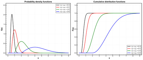
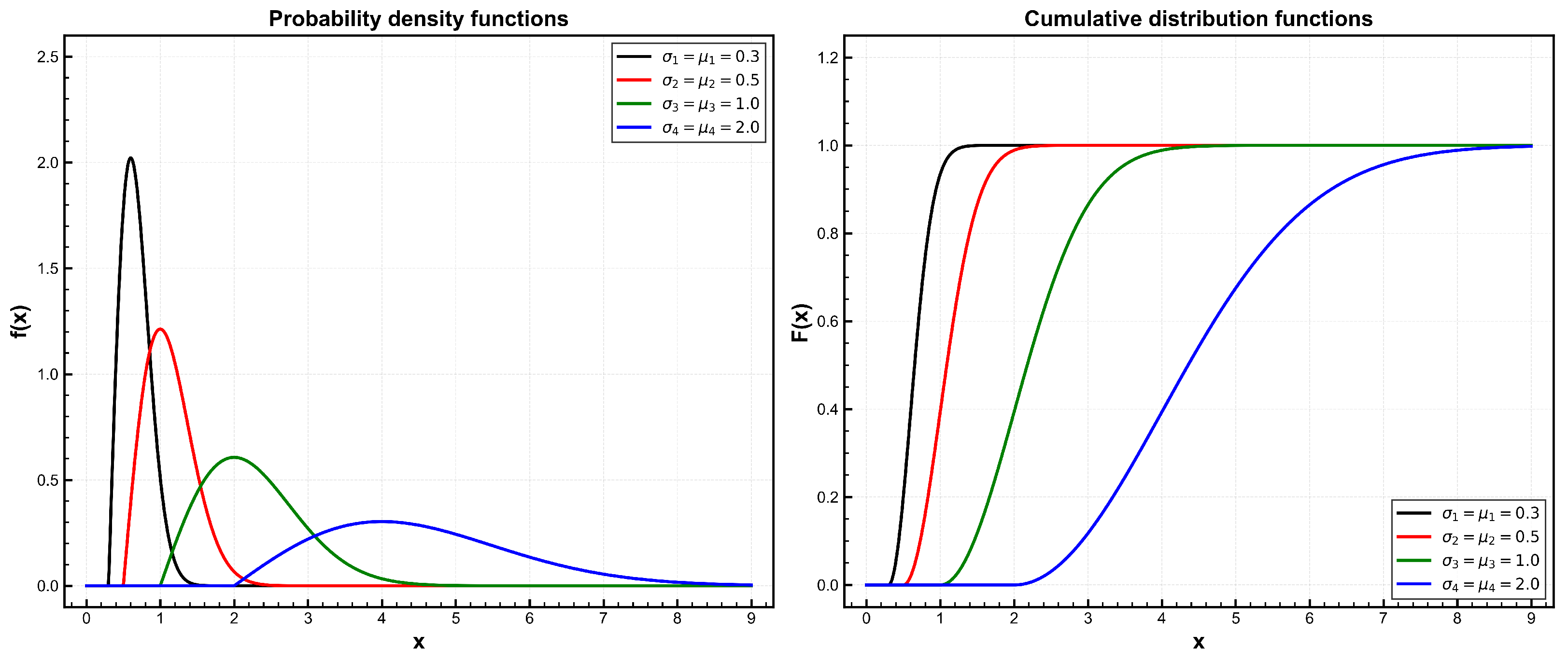
The two-parameter Rayleigh distribution offers greater flexibility than the standard Rayleigh distribution by incorporating a location parameter . This flexibility is particularly important in modeling scenarios where lifetime measurements do not originate from zero. Furthermore, the two-parameter Rayleigh distribution is invariably uni-modal and is characterized by an increasing hazard rate function. This renders it particularly well-suited for modeling the lifetime distributions of components subject to rapid aging over time. The probability density function and cumulative distribution function of this distribution are plotted in Figure 1.
Figure 1.
Left: probability density functions (PDFs) of the two-parameter Rayleigh distribution for (black), (red), (green), and (blue); right: corresponding cumulative distribution functions (CDFs).
Consider a test conducted on n specimens, where their individual lifetimes are denoted by . These random variables follow an independent and identical distribution, with the corresponding PDF and CDF .
Moreover, let represent the random censoring times for the aforementioned specimens, with their probability density function and cumulative distribution function given by and , respectively. For mathematical tractability, we assume that the failure time and the censoring time share the same location parameter . This simplification, which has been commonly adopted in the literature on random censoring (e.g., [12]), enables a clean derivation of the joint likelihood and preserves the two-parameter Rayleigh structure for the marginal distribution of . We further assume that and are mutually independent for each i. It is important to note that in practice, only one of and can be observed for each test unit. Let the actual observed time be denoted as for . In addition, an indicator variable is defined as follows:
Note that is a Bernoulli random variable whose probability mass function is defined as
The probability of failure prior to censoring is derived as follows:
Substituting this result gives the explicit marginal distribution:
Note that the expression for the above probability does not contain . To see that and are independent, consider the transformed variables and . Under the assumptions that and are independent and share the same location parameter , it follows that and are independent and follow exponential distributions. Specifically, and .
A classical result for exponential distributions (see [12]) states that, for two independent exponential variables, U and V, the event is independent of . Applying this result to and , we have that is independent of . Since , and is a one-to-one function of , it follows that and are independent.
Therefore, the joint probability distribution of can be expressed as
where the parameter is defined to simplify subsequent calculations.
The marginal distribution of can be obtained by summing the joint distribution in (2) over :
This is exactly the probability density function of a two-parameter Rayleigh distribution with location parameter and scale parameter , denoted as .
The expected values for and are derived as and , in that order. On this basis, the collection constitutes a random censoring sample, for which the joint probability function is elaborated in (2), and the respective marginal distributions are formulated by the mathematical expressions presented in (1) and (2).
3. Classical Estimation Methods
Maximum likelihood estimation (MLE) is employed to infer the unknown model parameters, where the ensuing analytical procedures are conducted on the basis of a randomly censored sample designated as . The likelihood function associated with this sample is formulated as follows:
Now, the log–likelihood function becomes
The likelihood is an increasing function of and is less than or equal to . Consequently, the MLE of the parameter is exactly given by . Note that is a boundary estimator, as it coincides with the smallest observation, while the true parameter is strictly less than all realizations of . Consequently, this estimator exhibits positive bias in finite samples, with its expectation given in Proposition 1 as . The bias decreases as the sample size n increases, confirming the consistency of .
Taking , . The MLEs corresponding to parameters and can be derived by numerically solving these two associated equations and as
3.1. Variance in the Maximum Likelihood Estimator
Proposition 1.
Let denote independent and identically distributed random variables that share a common probability density function
Then the minimum order statistic follows a two-parameter Rayleigh distribution with location parameter μ and scale parameter , i.e.,
Proof.
The CDF corresponding to (6) is
For the minimum of n independent random variables, we have
Expression (9) coincides with the cumulative distribution function of a two-parameter Rayleigh distribution having location and scale . Differentiating (9) with respect to gives the corresponding probability density function
This density matches precisely the form of a Rayleigh density with parameters and .
Consequently, it follows that , which thereby completes the theoretical proof. □
Since follows , the mean and variance in the are
Note that is a consistent but biased estimator of . By estimating with the sample minimum, the original three-parameter estimation problem reduces to a two-parameter problem involving only and , simplifying subsequent inference.
The second-order partial derivatives, needed for the observed Fisher information matrix, are
It is worth acknowledging that the maximum likelihood estimator of lies on the boundary of the parameter space, which may affect the regularity conditions underlying the Fisher information matrix. However, the MLE of is super-consistent and converges at rate n, which mitigates its impact on the asymptotic distribution of and . Nevertheless, the Fisher information matrix derived below focuses on the scale parameters and , which are interior points, and the resulting asymptotic intervals are commonly used in practice as approximations.
From (1), we have
For the Rayleigh distribution, it can be shown that
Now, the Fisher information matrix for can be derived as
Since the Fisher information matrix is diagonal here, it can be conveniently inverted by simply inverting each element along its main diagonal. The diagonal elements of the inverse information matrix provide the asymptotic variance estimators for the maximum likelihood estimators (MLEs). Specifically, these variance estimates are given by
These variance expressions depend on the unknown parameters and . For practical application, usable estimates of the variances are obtained by replacing and with their corresponding MLEs. The estimated variances for the estimators and are subsequently derived as follows:
3.2. Asymptotic Confidence Intervals
Given that follows a distribution, the two-sided equal-tailed confidence interval of for the parameter can be readily deduced in accordance with the method presented in reference [12]. Let
Then, the confidence interval (CI) of is
where denotes the upper critical value of Snedecor’s F-distribution with numerator and denominator degrees of freedom equal to 2 and , respectively. Herein, serves as the confidence coefficient, with the parameter satisfying the constraint that .
This interval construction assumes that is sufficient and that the data are exactly follow the two-parameter Rayleigh distribution. Under model misspecification, the actual coverage probability may differ from the nominal level. In such cases, bootstrap methods offer a more robust alternative for interval estimation of .
For the scale parameters and , the asymptotic sampling distribution associated with the MLEs follows a bivariate normal distribution denoted as . On this basis, we are able to derive the CI for the parameters by means of the normal approximation method. The two-sided CI corresponding to and can be expressed as
Here, refers to the upper th quantile of the standard normal distribution. It should be noted that these confidence intervals are based on asymptotic normal approximations, which may not be accurate for small or moderately sized samples, especially under heavy censoring. In practice, alternative methods such as bootstrap confidence intervals could be considered to potentially improve coverage accuracy in such scenarios.
In Section 6, we carry out a Monte Carlo simulation experiment to calculate the upper and lower confidence bounds of the parameters as well as the average lengths of their confidence intervals by using simulated samples, and further obtain the corresponding coverage probabilities for these intervals accordingly.
3.3. Method of Moments
Upon equating sample moments with the corresponding population moments, the relevant estimates of the model parameters are obtainable via this moment-matching approach. For the random variables D and Y, we define their sample counterparts based on the observed data as follows: , , and population moments , , . By equating the respective moments to one another, we thus obtain
We can derive the moment estimators corresponding to each parameter as
It can be observed that these moment estimators provide unique solutions for , , and since the sample moments satisfy and in practice. This indicates that the parameters are identifiable from the chosen moments.
3.4. Least-Squares Estimates
denote the order statistics from the marginal distribution of Y, where Y obeys a two-parameter Rayleigh distribution with location parameter and scale parameter . The parameter is defined as . The cumulative distribution function (CDF) corresponding to the random variable Y is expressed as
The expected value of is approximately
The least-squares estimates of the parameters , , and can be obtained by minimizing the following objective function
To account for the heterogeneity in the variances of , we consider the weighted least-squares method. The variance in is approximately
Taking the weights as , the weighted least-squares estimates are acquired through the minimization of
The minimization is carried out for , , and , where .
4. Bayesian Estimation
We proceed to develop a Bayesian inferential framework for the unknown parameters associated with the two-parameter Rayleigh distribution, where the whole analytical process is based on randomly censored data. On this basis, we derive the Bayes estimators for the aforementioned parameters under the generalized entropy loss function (GELF), as well as the associated highest posterior density (HPD)-credible intervals corresponding to each parameter. We then advance the Bayesian inference method for and with randomly censored data as the research basis; specifically, we impose the prior assumption that and , respectively, follow conjugate inverse gamma distributions with hyperparameters and , and the corresponding PDF are expressed as
For the location parameter , we introduce the subsequent improper uniform prior distribution
The parameters , , and are assumed to be independent priori.
The joint posterior distribution is
where .
This joint posterior density function does not admit an explicit closed form. Therefore, to compute the Bayes estimates, one may employ a numerical integration procedure based on the posterior distribution given in (17) under an appropriate loss function. Alternatively, the importance sampling algorithm can be employed to acquire simulation-consistent Bayesian estimators and construct the corresponding HPD-credible intervals, in accordance with the methodological approach introduced by [14].
To implement the Gibbs sampling procedure, we employ a technique analogous to that described by [15]. Setting , we take the posterior as
It follows that the joint posterior distribution can be written in the form of
where,
We note here that and correspond to inverse gamma density functions with a common scale parameter but different shape parameters and , respectively.
The density function is a valid proper density function. Its cumulative distribution function (CDF) can be derived as
This CDF is readily invertible, allowing for straightforward generation of random samples for via the probability integral transform. Specifically, for a uniform random variate , we can obtain a sample of by solving
Since the prior for is now defined on the finite interval , it is a proper prior. Together with the proper priors for and , the joint posterior distribution is guaranteed to be proper, ensuring the validity of Bayesian inference even for small sample sizes. This invertibility facilitates the implementation of the Gibbs sampling procedure.
4.1. Bayes Estimates Under GELF
For Bayesian estimation, we employ the generalized entropy loss function (GELF). Although this loss function was introduced earlier [16], it remains relevant in modern reliability analysis, as demonstrated in recent Bayesian studies on lifetime distributions under various censoring schemes [13,17]. The generalized entropy loss function is defined as follows:
Here, is an estimate of . For , underestimation incurs a more severe penalty than overestimation, whereas for , the situation is reversed, with overestimation being penalized more heavily. In particular, corresponds to the entropy loss function (ELF), corresponds to the squared error loss function (SELF), and corresponds to the precautionary loss function (PLF). These values represent different degrees of asymmetry and allow us to comprehensively assess the impact of the loss function on Bayesian estimates.
Within the Bayesian estimation framework, we select the value that minimizes the risk function . Deriving the Bayes estimator of involves computing the derivative of with respect to and equating the derived expression to zero. The Bayes estimator for and its related risk function are formulated as
We can also characterize Bayesian estimation of and under the GELF.
Although the improper uniform prior is used for the location parameter , the resulting joint posterior distribution remains proper. This can be seen by noting that the likelihood function in (3) contains the factor , which is bounded on the interval since . The exponential term is also bounded on this interval. Hence, the likelihood, viewed as a function of , is bounded on the truncated support .
Moreover, the constraint imposed by the observed data truncates the support of to the finite interval . Over this compact set, the bounded likelihood combined with the proper inverse gamma priors for and ensures that the joint posterior is integrable. More formally,
because:
- is bounded in on ;
- and are proper inverse gamma densities;
- The improper prior integrates to a finite constant over the finite interval .
Consequently, the joint posterior is well-defined and valid for Bayesian inference.
4.2. Gibbs Sampling Procedure
The Gibbs sampling algorithm (Algorithm 1), which is used to generate samples from the joint posterior distribution , is implemented as follows:
| Algorithm 1 Gibbs Sampling for Bayesian Estimation under GELF. |
Require: Initial values ; hyperparameters ; total iterations M; burn-in period B; loss function parameter
|
When no prior information is available, we can employ non-informative prior distributions for the relevant parameters. For the scale parameters and , this corresponds to setting in the inverted gamma priors. For the location parameter , we retain the improper uniform prior . Under these non-informative priors, the posterior distribution is dominated by the likelihood.
Convergence of the Gibbs sampler was assessed using trace plots and the Gelman–Rubin diagnostic. We ran three parallel chains with over-dispersed starting values, each for M = 20,000 iterations, discarding the first iterations as burn-in. In all cases, values were below 1.1, indicating that convergence was achieved. The effective sample sizes (ESSs) for all parameters exceeded 1000, ensuring reliable posterior inference.
4.3. HPD-Credible Intervals and Chen–Shao Algorithm
A highest posterior density (HPD) credible interval is defined to be an interval that fulfills the two subsequent criteria: it contains a posterior probability mass of , and the posterior density at every interior point within the interval exceeds that at all exterior points outside the interval. As a result, the HPD interval is the shortest credible interval achievable for a specified probability level of . Based on these basic properties, ref. [14] proposed a computational procedure for deriving the HPD-credible interval corresponding to the parameter .
The Chen–Shao algorithm [14] is given in Algorithm 2.
| Algorithm 2 Finding the HPD-credible interval. |
Require: MCMC total iterations M, burn-in period B, significance level
|
The same procedure can be applied to obtain HPD-credible intervals for and . Specifically, after obtaining the posterior samples and from the Gibbs sampling algorithm, we sort each set of samples in ascending order and apply Steps 2–3 of Algorithm 2 to find the shortest intervals that contain the desired posterior probability. This yields the HPD-credible intervals for and , respectively.
5. Reliability and Experimental Characteristics Estimation
Within the present analytical framework, the two-parameter Rayleigh distribution parameterized by is employed to model lifetime data, while its reliability metrics and experimental behavior are examined using the corresponding estimators derived under a randomly censored sampling scheme.
A key practical consideration is whether a life test can be finished within a predefined time interval. As experimental costs depend directly on the test duration, this information is key to selecting a suitable sampling strategy and determining the sample size for life test specimens.
In random censoring model, the observed time follows a two-parameter Rayleigh distribution , where . The completion time of the experiment is determined by the maximum observed value, i.e., .
The cumulative distribution function of is
The expected time on test (ETT) is defined as the expectation of
For the Rayleigh distribution, this integral lacks a straightforward closed-form expression yet can be solved via numerical methods. In practice, the observed time on test (OBTT), which is itself, serves as a natural estimator of ETT.
For the complete data (no censoring) scenario, the test time is determined by the maximum failure time , and its expected value is
where are the posterior samples obtained through Gibbs sampling, and is computed using Equation (24).
Since the expected time on test does not have a closed-form expression for the Rayleigh distribution, both and require numerical integration. For each parameter set , we compute the integral in Equation (24) using adaptive numerical integration methods. In the Bayesian framework, this computation is performed for each posterior sample , and the results are then combined according to Table 1.
Table 1.
Maximum likelihood estimates and Bayesian estimates under GELF of reliability and experimental characteristics.
For the numerical computation of the expected time on test (ETT), we employed adaptive numerical integration as implemented in the R integrate function. The integration was performed over the interval , which was verified to capture the essential support of the distribution. The relative tolerance was set to (for estimation) and (for true value computation), with subdivisions up to 1000 to ensure accuracy. Based on our implementation, the computational cost of a single ETT evaluation is approximately 0.002 s on a standard desktop computer. In the simulation study with 10 parameter combinations, three sample sizes (), and replications per configuration, the total time for ETT estimation was approximately 0.2 min, which was negligible compared to the overall computational burden.
6. Simulation Studies
A Monte Carlo simulation experiment is carried out to assess and compare the performance of the various estimators proposed previously. Specifically, to facilitate a direct comparison between classical and Bayesian inference methods, we generate randomly censored samples across a range of values for parameters , , and . For each generated sample, we calculate the MLEs along with their respective confidence intervals. Besides the Bayes estimators derived under the generalized entropy loss function, along with the associated HPD-credible intervals corresponding to such estimators.
Before detailing the simulation procedure, we clarify the selection of hyperparameters for informative priors. They are chosen so that the prior means equal the true parameter values (i.e., and ), ensuring that the prior information is centered correctly. This allows for a meaningful evaluation of the Bayesian estimators’ performance when prior information is accurate.
We now outline the simulation procedure step-by-step as Algorithm 3.
| Algorithm 3 Monte Carlo simulation procedure. |
|
To compare the performance of the Bayesian estimation method and the classical estimation method, we try different parameter values and hyperparameter values, with the primary simulation results shown in Table 2, Table 3, Table 4, Table 5, Table 6 and Table 7.
Table 2.
MLEs for the parameters with different sample sizes.
Table 3.
Expected time on test (ETT) estimates under different methods.
Table 4.
Bayesian estimates under the SELF for the parameters.
Table 5.
Least-squares (LS) and weighted least-squares (WLS) estimates for the parameters.
Table 6.
Bayesian estimates under the non-informative prior for the parameters.
Table 7.
Interval estimation results with different sample sizes.
Based on the comprehensive analysis of the results presented in the aforementioned tables, it can be concluded that
- Maximum likelihood estimation: MLE exhibits systematic bias that decreases with increasing sample size. The bias is more pronounced in small samples, while both bias and MSE improve significantly as sample size increases, confirming the consistency property of MLE but also highlighting its limitations in small-sample scenarios.
- Least-squares and weighted least-squares: Both LS and WLS methods provide reasonable parameter estimates across all sample sizes. For small samples (), LS and WLS show notable bias, particularly for the scale parameters and , with MSE values considerably larger than those of MLE and Bayesian methods. However, as sample size increases to and , the performance of both methods improves substantially, with bias and MSE decreasing markedly. WLS generally yields slightly lower MSE than LS for most parameter combinations, particularly for larger parameter values, confirming the benefit of incorporating variance heterogeneity in the estimation procedure.
- Expected time on test (ETT): The ETT estimates exhibit similar patterns to the parameter estimates, with bias and MSE decreasing as sample size increases. For , the ETT estimates show considerable bias, especially for combinations with larger parameter values. However, the bias is substantially reduced for and , with MSE decreasing by approximately 50% to 70% compared to the small sample case, indicating that reliable ETT estimation requires moderate to large sample sizes. The numerical integration procedure proved to be both accurate and computationally efficient, with negligible impact on overall simulation time.
- Comparison of Bayesian methods: The SELF estimator outperforms both MLE and non-informative priors across all sample sizes, with its advantage being most pronounced in small samples. Although this advantage diminishes as sample size increases, it remains present, indicating that informative priors provide crucial stability when data are scarce.
- Effect of prior information: Non-informative priors perform reasonably well but yield larger MSEs than SELF, with the difference being more substantial in small samples. As sample size increases, the gap narrows considerably. This demonstrates that the advantage of Bayesian methods stems primarily from the informative prior structure, and this benefit is most prominent when sample information is limited.
- Interval estimation: The asymptotic confidence intervals for , , and show coverage probabilities that improve with increasing sample size. For , the coverage probabilities are below the nominal 95% level for all parameters, particularly for . As sample size increases to and , coverage probabilities approach the nominal level for and show improvement for and , although some undercoverage remains. Interval lengths decrease consistently with increasing sample size, as expected. These results suggest that caution is warranted when interpreting confidence intervals in small samples, especially for the scale parameters.
- Sample size effects: The most dramatic improvement across all estimators occurs between small and moderate sample sizes, with diminishing returns thereafter. This suggests that a moderate sample size provides a reasonable balance between estimation accuracy and experimental cost in practical applications.
- Practical recommendations: Based on the systematic comparison across sample sizes, we recommend prioritizing Bayesian methods such as SELF for small samples; for moderate samples, SELF remains the preferred choice while non-informative priors and LS/WLS methods serve as viable alternatives; for large samples, all methods are acceptable, though Bayesian methods still offer some efficiency gains. For ETT estimation, moderate to large sample sizes () are recommended to achieve reliable results. The interval estimation method for becomes reliable for , but caution is advised when interpreting and intervals, particularly in small samples.
To assess the impact of the loss function parameter on the Bayesian estimates, we compare the results obtained under three different loss functions: SELF (), ELF (), and PLF (). Table 6 presents the parameter estimates for selected parameter combinations with sample size .
The results in Table 8 show that the parameter estimates are relatively stable across different loss functions. The differences between SELF, ELF, and PLF are generally small, with slightly larger variations observed for PLF in some cases (e.g., for in the (5,5,3) combination). This indicates that the Bayesian estimation procedure is robust to the choice of the loss function parameter within a reasonable range.
Table 8.
Sensitivity analysis for different loss functions ().
To provide a structured comparison, Table 9 presents the relative efficiency (RE = MSE_SELF/MSE_MLE) for selected parameter combinations. Values less than 1 indicate that SELF outperforms MLE.
Table 9.
Relative efficiency for selected parameter combinations.
The results show that all RE values are below 1, confirming the consistent superiority of Bayesian methods across all scenarios. The improvement is most pronounced for and estimation, with RE values as low as 0.04, and becomes more evident as sample size increases.
7. Real Data Example Analysis
To further validate the practical applicability of the proposed methodological framework, an illustrative empirical analysis is conducted herein by utilizing a carbon fiber strength dataset first published in the work of [15]. This dataset documents the strength values of individual carbon fibers as well as impregnated 1000-carbon fiber tows, with the full set of experimental data tabulated in Table 10. In line with the goodness-of-fit verification tests and the scaled total time on test (TTT) transformation method put forward by [15], the Rayleigh distribution is verified to be a suitable probabilistic model for characterizing the statistical properties of this carbon fiber strength dataset.
Table 10.
Strength data.
This analysis aims to show the superior precision of the location-scale Rayleigh model over the standard scale-only version. We consider model fitting for the dataset using: (i) a two-parameter Rayleigh model (, ) and (ii) a one-parameter Rayleigh model (), with parameters estimated by maximum likelihood. The goodness of fit for these models is then evaluated based on several metrics: negative log–likelihood, Akaike Information Criterion (AIC), Bayesian Information Criterion (BIC), the Kolmogorov–Smirnov (K–S) statistic, and the empirical cumulative distribution function (ECDF).
For the K-S test, the null hypothesis is that the observed randomly censored data follow the specified Rayleigh distribution. A small p-value (typically ) leads to the rejection of , suggesting that the distributional assumption may not be appropriate.
The formula for calculating AIC is as follows:
where k denotes the number of parameters incorporated into the statistical model, and L represents the maximum likelihood value associated with the estimated model.
The BIC is mathematically expressed as
where k and L retain their definitions from the AIC formula, and n refers to the total number of observations in the dataset (Table 11 and Table 12).
Table 11.
Parameter estimates.
Table 12.
Fitting summary statistics for the model.
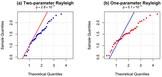
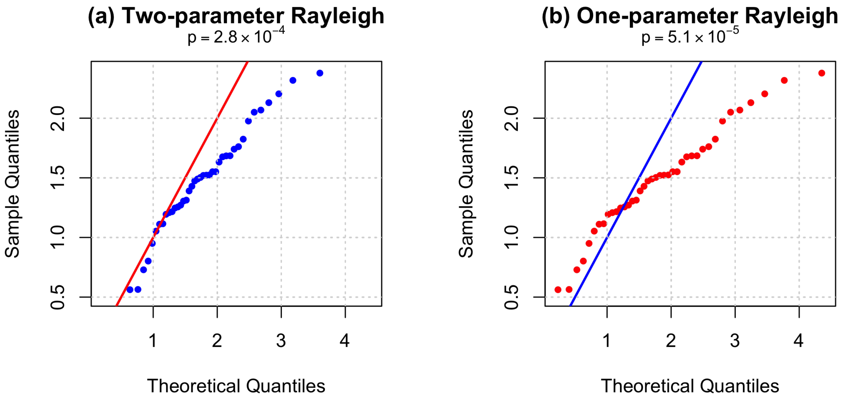
It should be noted, however, that although the two-parameter Rayleigh distribution provides a better fit than its one-parameter counterpart, the Kolmogorov–Smirnov test yields p-values below 0.05 for both models, indicating that neither fully captures the empirical distribution of the carbon fiber strength data at conventional significance levels. This suggests that while the two-parameter model offers a substantial improvement, there may still be room for further refinement, such as considering more flexible distributions or mixture models. Q-Q plots are provided in Figure 2, which visually confirm the improved fit of the two-parameter model. Although both models show significant deviation from the 45-degree line (K-S test ), indicating imperfect fit, the two-parameter model demonstrates noticeably better alignment, particularly in the upper tail. This superior fit is consistent with its lower AIC and BIC values in Table 12, confirming that the inclusion of a location parameter improves model performance even when the overall fit is not ideal.
Figure 2.
Q-Q plots for (a) two-parameter and (b) one-parameter Rayleigh distributions based on failure times.
Based on all goodness-of-fit criteria, we find that the two-parameter Rayleigh distribution achieves substantially lower values of negative log–likelihood, AIC, and BIC compared to the one-parameter Rayleigh distribution. Therefore, the two-parameter Rayleigh distribution exhibits markedly superior fitting performance to the one-parameter Rayleigh distribution.
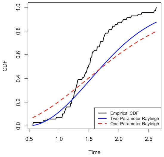
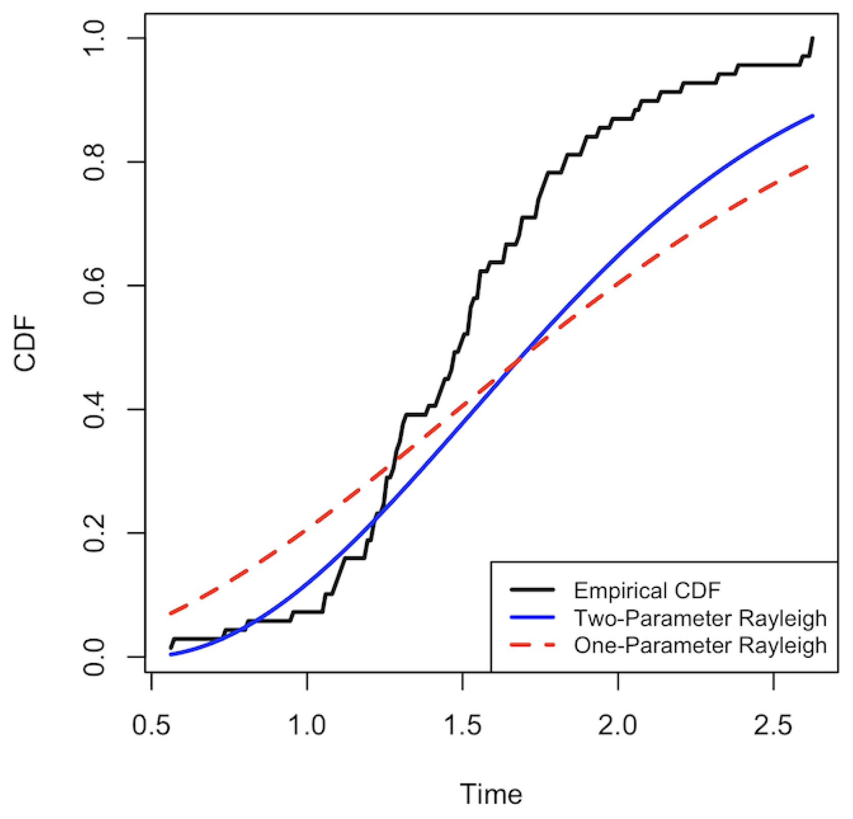
For the graphical comparison, we present the cumulative distribution curves and examine their respective behaviors. As shown in Figure 3, the CDF curve of the two-parameter Rayleigh distribution lies closer to the empirical CDF than that of the one-parameter model. Consequently, we conclude that fitting this real dataset with the two-parameter Rayleigh distribution yields a considerably better fit than the one-parameter Rayleigh distribution, which only includes a scale parameter.
Figure 3.
CDF curves for the strength data. ECDF of the strength data (black), fitted CDFs from the two-parameter (red) and one-parameter (blue) Rayleigh distributions.
8. Conclusions
Randomly censored data are commonly encountered in both survival analysis and reliability theory. Numerous statistical distributions have been extensively utilized in prior research to develop estimation procedures under this data framework. This study introduces location parameter modeling into the analysis of randomly censored data following the Rayleigh distribution, thereby establishing a novel analytical framework for lifetime processes characterized by monotonically increasing failure rates. The inclusion of a location parameter is expected to influence estimates derived from data. The core objective of this study is to integrate this location parameter into models for both lifetime and censoring time distributions.
This study investigates a diverse set of estimation approaches for the location and scale parameters within the framework of the two-parameter Rayleigh distribution. A number of classical estimation methods are explored herein. In addition, Bayesian estimators corresponding to the parameters, as well as their CIs and HPD-credible intervals, are constructed under multiple loss functions. Given the theoretical challenges associated with comparing different estimation methods, a Monte Carlo simulation study is conducted to assess the performance of the various parameter estimators and their associated reliability characteristics. Comparisons among these estimators are mainly based on two key metrics: bias and mean squared error. Owing to the integration of supplementary prior information, Bayesian estimators can generate more accurate results than maximum likelihood estimators (MLEs) in certain cases, especially when the parameter values are large and the sample sizes are small. To demonstrate the practical applicability of the estimation methodologies proposed in this study, a real-world case analysis is presented using carbon fiber strength data. The empirical results show that the fitting performance of the two-parameter Rayleigh distribution is significantly superior to that of its one-parameter counterpart.
Future research could relax the assumption that failure and censoring times share the same location parameter, allowing these two processes to have different location parameters. Furthermore, the modeling framework of the two-parameter Rayleigh distribution could be extended to more complex survival analysis scenarios. For instance, covariates could be introduced to establish regression models, thereby analyzing the influence of various factors on lifetime distributions. Alternatively, the distribution could be integrated with structures such as competing risks or frailty models to handle more complex failure mechanisms and heterogeneous data.
Author Contributions
Conceptualization, L.Z.; Methodology, L.Z. and Z.Z.; Software, L.Z., Z.Z. and M.L.; Validation, Z.Z.; Formal analysis, L.Z.; Investigation, L.Z.; Resources, M.L.; Data curation, M.L.; Writing—original draft, L.Z.; Writing—review & editing, W.G.; Visualization, M.L.; Supervision, W.G.; Project administration, W.G. All authors have read and agreed to the published version of the manuscript.
Funding
This research was supported by Project 202610004010 which was supported by National Training Program of Innovation and Entrepreneurship for Undergraduates. Wenhao’s work was partially supported by the Science and Technology Research and Development Project of China State Railway Group Company, Ltd. (No. N2023Z020).
Data Availability Statement
The original contributions presented in this study are included in the article. Further inquiries can be directed to the corresponding author.
Conflicts of Interest
The authors declare that this study received funding from the Science and Technology Research and Development Project of China State Railway Group Company, Ltd. (No. N2023Z020). The funder was not involved in the study design, collection, analysis, interpretation of data, the writing of this article or the decision to submit it for publication.
Notation
The following notations are used throughout this paper.
| Symbol | Description |
| Location parameter (minimum lifetime) | |
| Scale parameter for failure time distribution | |
| Scale parameter for censoring time distribution | |
| Significance level (e.g., in confidence intervals) | |
| Censoring indicator ( if failure observed, 0 otherwise) | |
| Observed time, | |
| Number of failures, | |
References
- Banerjee, P.; Bhunia, S.; Seal, B. Partial Bayes Estimation in Two-Parameter Rayleigh Distribution. Am. J. Math. Manag. Sci. 2024, 43, 123–140. [Google Scholar] [CrossRef] [Scilit]
- Dey, T.; Dey, S.; Kundu, D. On Progressively Type-II Censored Two-Parameter Rayleigh Distribution. Commun. Stat.-Simul. Comput. 2016, 45, 438–455. [Google Scholar] [CrossRef] [Scilit]
- Luo, L.; Ma, Z.; Wang, M. Robust explicit estimators of the shifted Rayleigh distribution under Type II censoring. J. Reliab. Eng. Qual. Manag. 2025, 17, 117–130. [Google Scholar] [CrossRef] [Scilit]
- Ghitany, M.E. A compound Rayleigh survival model and its application to randomly censored data. Stat. Pap. 2001, 42, 437–450. [Google Scholar] [CrossRef] [Scilit]
- Ghitany, M.E.; Al-Awadhi, S. Maximum likelihood estimation of Burr XII distribution parameters under random censoring. J. Appl. Stat. 2002, 29, 955–965. [Google Scholar] [CrossRef] [Scilit]
- Friesl, M.; Hurt, J. On Bayesian estimation in an exponential distribution under random censorship. Kybernetika 2007, 43, 45–60. [Google Scholar]
- Abu-Taleb, A.A.; Smadi, M.M.; Alawneh, A.J. Bayes estimation of the lifetime parameters for the exponential distribution. J. Math. Stat. 2007, 3, 106–108. [Google Scholar] [CrossRef] [Scilit]
- Danish, M.Y.; Aslam, M. Bayesian estimation for randomly censored generalized exponential distribution under asymmetric loss functions. J. Appl. Stat. 2013, 40, 1106–1119. [Google Scholar] [CrossRef] [Scilit]
- Danish, M.Y.; Aslam, M. Bayesian inference for the randomly censored Weibull distribution. J. Stat. Comput. Simul. 2014, 84, 215–230. [Google Scholar] [CrossRef] [Scilit]
- Krishna, H.; Vivekanand, K.K. Estimation in Maxwell distribution with randomly censored data. J. Stat. Comput. Simul. 2015, 85, 3560–3578. [Google Scholar] [CrossRef] [Scilit]
- Garg, R.; Dube, M.; Kumar, K.; Krishna, H. On randomly censored generalized inverted exponential distribution. Am. J. Math. Manag. Sci. 2016, 35, 361–379. [Google Scholar] [CrossRef] [Scilit]
- Krishna, H.; Goel, N. Classical and Bayesian inference in two parameter exponential distribution with randomly censored data. Comput. Stat. 2018, 33, 249–275. [Google Scholar] [CrossRef] [Scilit]
- Chaturvedi, A. Randomly Censored Kumaraswamy Distribution. J. Stat. Theory Appl. 2024, 23, 1–25. [Google Scholar] [CrossRef] [Scilit]
- Chen, M.H.; Shao, Q.M. Monte Carlo estimation of Bayesian credible and HPD intervals. J. Comput. Graph. Stat. 1999, 8, 69–92. [Google Scholar] [CrossRef] [Scilit]
- Dey, S.; Dey, T.; Kundu, D. Two-parameter Rayleigh distribution: Different methods of estimation. Am. J. Math. Manag. Sci. 2014, 33, 55–74. [Google Scholar] [CrossRef] [Scilit]
- Calabria, R.; Pulcini, G. Point estimation under asymmetric loss functions for left-truncated exponential samples. Commun. Stat.-Methods 1996, 25, 585–600. [Google Scholar] [CrossRef] [Scilit]
- Kumari, A.; Kumar, K.; Kumar, I.B. Bayesian and Classical Inference in Maxwell Distribution Under Adaptive Progressively Type-II Censored Data. Int. J. Syst. Assur. Eng. Manag. 2023, 15, 1015–1036. [Google Scholar] [CrossRef] [Scilit]

Disclaimer/Publisher’s Note: The statements, opinions and data contained in all publications are solely those of the individual author(s) and contributor(s) and not of MDPI and/or the editor(s). MDPI and/or the editor(s) disclaim responsibility for any injury to people or property resulting from any ideas, methods, instructions or products referred to in the content. |
© 2026 by the authors. Licensee MDPI, Basel, Switzerland. This article is an open access article distributed under the terms and conditions of the Creative Commons Attribution (CC BY) license.