


Abstract
The isotropic Cauchy distribution is a member of the central -stable family that plays a role in the set of heavy-tailed distributions similar to that of the Gaussian density among finite second-moment laws. Given a sequence of n observations, we are interested in characterizing the performance of Likelihood Ratio Tests, where two hypotheses are plausible for the observed quantities: either isotropic Cauchy or isotropic Gaussian. Under various setups, we show that the probability of error of such detectors is not always exponentially decaying with n, with the leading term in the exponent shown to be logarithmic instead, and we determine the constants in that leading term. Perhaps surprisingly, the optimal Bayesian probabilities of error are found to exhibit different asymptotic behaviors.
1. Introduction
Detecting the underlying sampling distribution of an empirical set of n observations is a challenging and fundamental question in statistics. It falls under the family of hypothesis testing problems whenever deciding on a possibility among a given number of choices. In the binary scenario (p vs. q), it is well known that Likelihood Ratio Test (LRT) detectors are optimal for multiple setups. Under a Neyman–Pearson criterion or under a Bayesian risk formulation, the performance of such detectors is expected to be exponentially decaying with n, with the exponent being a Kullback–Leibler (KL) distance between pertinent laws. This is the case in a discrete scenario [1] (Th. 11.8.3 & Th. 11.9.1), where a well-known proof is based on the method of types. Extensions to continuous setups do exist under certain conditions [2,3].
One interesting quest is to analyze this decision problem while testing for:
- The Cauchy distribution: representative of the family of “heavy-tailed” -stable distributions versus;
- The Gaussian distribution: a central model among finite-variance probability laws.
Note that both models are limiting distributions of Independent and Identically Distributed (IID) sums of Random Variables (RV)s by the results of the generalized Central-Limit Theorem [4] and are therefore supported by strong theoretical evidence whenever the observations are the result of the accumulation of a large number of random independent events. While the Gaussian model has been dominant in the literature, with both theoretical and empirical justifications, recent studies suggested the non-suitability of the Gaussian models and proposed heavy-tailed ones including the -stable family in a multitude of scenarios: interference modeling in digital communication [5,6], radar clutter data [7], internet traffic modeling [8], and financial data [9] among many other examples that can be found in [10,11]. In the multivariate case, random feature models are used to better understand several complex behaviors of neural networks [12,13,14]. In [15], the authors consider the problem of classification features in high dimensions by assuming a heavy-tailed data model according to a superstatistical construction [16]: the feature vector is assumed to be distributed according to , where is multivariate Gaussian with IID components, and Z is a positive RV. This defines a dependent statistical model for the observed data and has been found suitable in many other instances [17,18].
Among the isotropic (we will use “circular” interchangeably with “isotropic” in this document) multivariate -stable densities that follow the superstatistical construction [19] (p. 78 Definition 2.5.1), the isotropic Cauchy is the only distribution that has a closed-form Probability Density Function (PDF). With a view towards developing a suitable working framework with tractable results, we tackle in this work the problem of testing the n-dimensional isotropic Cauchy distribution hypothesis (heavy-tailed dependent features) versus the n-dimensional isotropic Gaussian one (independent features). More specifically, given a sample of n observations sampled from a rotationally invariant density, we want to characterize the error limits of the LRT devices detecting whether the observations are circular Gaussian, with PDF denoted , or circular Cauchy, with PDF . We note that the proposed setup is substantially different from the standard one regarding two main aspects:
- First, circular Cauchy vectors are statistically dependent (correlated) (whenever the usual notion of correlation is not well defined, such as for Cauchy variables, for example; we use the term “correlated” in this document to refer to statistical dependence) and not independent, as is the case for a Gaussian vector.This can be readily seen through multiplying two Cauchy PDFs, for example, and noting that the joint law is not an exclusive function of the norm. This indicates that a Cauchy vector with independent components is not circular.
- Second, the relative entropy is infinite, as shown in Appendix A.
Correspondingly, the results are found to deviate from the norm regarding two aspects:
- First, we show that the probability of error is not exponentially small with n. Namely, we prove that, under a Neyman–Pearson formulation and in the first order of the exponent, the leading term is linear for the error of the first kind () but only logarithmic for that of the second kind (). A similar logarithmic behavior of the exponent of the leading term is shown for the Bayesian error. Whenever possible, we determine the multiplicative constants of the provided asymptotic expressions.
- Second, we observe that the two types of Bayesian errors do not possess the same asymptotic rate, which is at odds with the general assumption of a similar asymptotic behavior under IID statistics (see [1] (Th. 11.9.1]) for the discrete case). We postulate that this is due to the fact that the observations are correlated, and we support our observation by providing in Appendix B illustrative examples in which one of the two hypotheses is correlated.
The rest of this paper is organized as follows: we present the problem and the main results in the form of two theorems in Section 2. Derivation of the results use technical lemmas and are detailed in Section 3. Finally, Section 4 concludes the paper.
Notations
We adopt the following conventions. For two asymptotically positive functions, if for every , for n large enough. We also write if there exist and such that and for n large enough (this is sometimes written using the Knuth notation as ). Functions and are said to be “asymptotically equivalent” if ; we write .
2. Problem Formulation and Main Results
We consider the binary hypothesis testing problem where, given a (large) number of observations, we need to decide between the two hypotheses:
where circular denotes a zero-mean multivariate isotropic Gaussian vector with covariance matrix , being the identity matrix. In contrast, circular represents an isotropic Cauchy vector with parameter , which can be written under the form , where is a zero-mean Gaussian vector with IID components each with variance , and A is Lévy-distributed with a zero location parameter and a scale parameter equal to [19] (p. 78 Definition 2.5.1). We note that the components of the isotropic Cauchy vector are dependent.
Whether under a Bayesian risk formulation or a Neyman–Pearson criterion, the optimal device is known to be an LRT:
for some appropriately chosen . We note that as increases, both and increase.
Our objective is twofold. First, we study the optimal Bayesian device and characterize its overall probability of error at large values of n via computing the asymptotic behavior of the probabilities of error of type I and II, as captured by and , respectively. More specifically, if and denote the prior probabilities of and , respectively, in Theorem 1, we show that as , the probability of error of the optimal device is
Second, we adopt the Neyman–Pearson criterion and answer the following question: let , for some . What is the asymptotic behavior of of the optimal device as ? We show in Theorem 2 that
We also answer the same question for the inverted problem: if , we show in Theorem 2 that
For mathematical convenience and without loss of generality, we scale our observation vector by and we denote the constant by . The resulting equivalent problem is:
The PDFs and are given by
where .
We state our main results in the form of Theorems 1 and 2. We also provide in Appendix D precise numerical computations that align with the results of Theorems 1 and 2.
In a Bayesian setting, the probability of error is determined in the following theorem:
Theorem 1.
Consider a sequence of n observations and a binary decision problem with two hypotheses for their distribution: either circular (IID) Gaussian with prior probability or circular (correlated) Cauchy with prior probability .
Let , and . For the Maximum A Posteriori (MAP) detector, optimal under a Bayesian formulation,
Note that the optimal error probabilities and , the ones that minimize the Bayesian probability of error , exhibit asymptotic behaviors that are not symmetric. That symmetry is a known property of the optimal Bayesian detector under IID observations: In a discrete binary hypothesis testing setup, whenever are IID according to p with prior probability or q with prior probability , then both the type I and II error probabilities under the optimal test are asymptotically of the form , where is the Chernoff information [1]. This is not true in general under correlated settings as in Theorem 1. We provide additional examples in Appendix B, which also show that there are no guarantees under the correlated setup for to become infinitesimally small as the number of observations n increases.
Theorem 2.
Consider a sequence of n observations and a binary decision problem with two hypotheses for their distribution: either circular (IID) Gaussian or circular (correlated) Cauchy . Let , and consider an .
Let be the standard Gaussian Q-function (the function is defined as ) and be its inverse function. Under a Neyman–Pearson criterion, the optimal LRT detector is such that
- Case 1: whenever , , where .
- Case 2: whenever ,for some .
The results of Theorem 2 also depart from the standard results of the Chernoff–Stein lemma [1] (Thm. 11.8.3). That lemma states that under IID observations, setting the type I error probability to be no worse than , the type II error probability is asymptotically of the form , and hence exponentially decaying with n with a constant rate equal to the KL divergence between p and q, the two alternatives of the testing problem. In Theorem 2, Case 1 shows a polynomial decay and not an exponential one. We believe that this is due to having a correlated hypothesis. We prove in Appendix A that , thus suggesting an asymptotic expression of the type II error probability of the form , where , represent the joint probability distributions under n observations. This provides a generalization of the result of the Chernoff–Stein lemma under IID statistics.
The remainder of this document is dedicated to deriving the main results stated in Theorems 1 and 2.
3. Technical Proofs
3.1. Preliminaries
Define the left-hand side of Equation (1) as :
Whenever is greater or equal to , the LRT Equation (1) decides on the Gaussian hypothesis. As such, when computing and , the larger the value of is, the larger these probabilities.
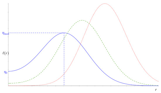
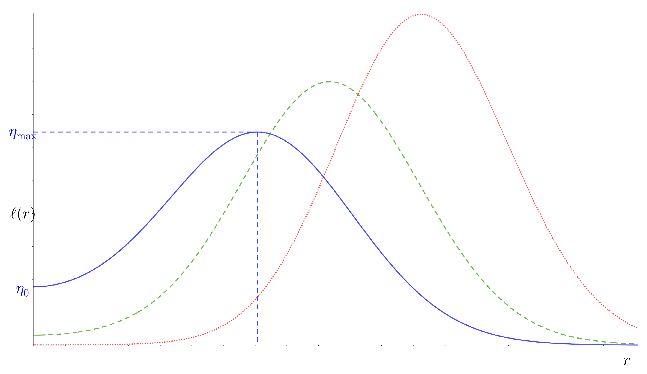
Characterizing the LRT problem (1) is naturally governed by the variations of and by the solution(s) of . Given a value of , has a peak and takes the general form depicted in Figure 1 whenever . Since we are interested in the asymptotic regime where n is very large, we assume that n is large enough for this condition to be true for any given value of . Under this regime, satisfies the following properties illustrated in Figure 1:
Figure 1.
for , with (solid blue), (dashed green), and (pointed red).
- Asymptotically, as .
- Its y-intercept, which we denote by , is equal to
- It peaks at , reaching a value of :
Using Stirling’s approximation, one can show:
and since is constant,
3.2. Operating Regime (OR)
Denote by
where the approximation is due to Equation (6), and let and denote the Lambert W function of branches 0 and , respectively. As can be seen in Figure 1, there are three regimes based on the value of the threshold in Equation (1): , , and . As it will turn out to be the case, the only “Operating Regime” (OR) for the problem at hand is the second one: , for which has two solutions,
We next compute and under the OR. We first compute :
where we used the change of variable to write the last equality. As for , we have:
where Equation (12) is due to the change of variable .
In order to determine the asymptotic behavior of both and at large values of n, it is imperative to first analyze the growth rate of the intersection points under the OR. We identify three cases:
- (i)
- : This includes, for example, the case of fixed. Equation (7) implies that and [20] (pp. 350–351)which giveswhereNote that in this case, since .
- (ii)
- (iii)
- , which implies . Whenever , the following approximations hold [20] (p. 350):
- For the remainder of this paper, we refer to the preceding three cases of the OR by (R-i), (R-ii), and (R-iii).
3.3. The Bayesian Detection Problem: Proofs
We start first by stating a technical lemma.
Lemma 1.
Whenever , the following hold:
where is the standard Gaussian Q-function.
Proof.
The detector is operating under Regime (R-i). Using the expression of in Equation (11), it is shown in Equation (A25) in Appendix C that:
which gives
where we used Equation (5) in order to write Equation (22). Equation (19) is due to Taylor’s approximation of the upper incomplete Gamma function around , and we used the fact that to write Equation (20). Equation (21) is due to Equation (14) and to the fact that
This concludes the first part of the proof. When it comes to , its expression is given by Equation (12):
where, in order to write the last equation, we used Stirling’s approximation
and the fact that:
as given by Equations (13) and (14). Equation (23) is due to applying the Laplace approximation method [21] around . This concludes the proof of the lemma. □
- Proof of Theorem 1 (Stated in Section 2)
Proof.
Since the MAP detector is an LRT Equation (1) for , for n large enough and fixed, the detector Equation (1) will be operating under Regime (R-i), and hence, the expressions of and of Lemma 1 do apply. Replacing by its asymptotic behavior as characterized by Equation (5) yields the required expression for . The same applies to after using the following approximation [22]:
This concludes the proof of Theorem 1. □
3.4. The Neyman–Pearson Formulation: Proofs
When it comes to the Neyman–Pearson criteria, we first estalish the following lemma:
Lemma 2.
For n large enough, the optimal Neyman–Pearson LRT detectors operate:
- under Regime (R-i) whenever ,
- under Regime (R-ii) whenever .
Proof.
Since increases with , in order for to be equal to as n grows to infinity, then must increase “as fast as ” with n, for otherwise, would go to zero, as implied by our analysis in Lemma 1 and our observations in Section 3. Moreover, since Equation (5), and , then by inspection, one can see that necessarily , which corresponds to Regime (R-i).
Similarly, is decreasing with and for a fixed . In order for to be equal to , must decrease with n. We prove next that Regime (R-iii) (and a fortiori ) is not possible, for otherwise, . In fact, Equation (A24) in Appendix C gives a lowerbound on :
where the limit result is due to Stirling’s identity and to the asymptotic behavior of and under Regime (R-iii) according to Equations (17) and (18). Furthermore, we show that must be under Regime (R-ii) by ruling out Regime (R-i) as well. Indeed, under case (R-i), the condition of Lemma 1 is satisfied, and hence,
where we used the fact that Equation (5). This rules out the Regime (R-i), thus proving our assertion. □
- Proof of Theorem 2 (Stated in Section 2)
Proof.
Let . We begin with the proof of Case 1. Whenever , the results of Lemma 2 imply that Regime (R-i) is the operating regime. Therefore, we use the result of Lemma 1 to write the expression of :
where is the inverse Q-function. Using the expression of as given in Lemma 1, we obtain:
where the last relation follows from Equations (5) and (26). This completes the proof of Case 1.
We move now to proving Case 2 of the theorem. As shown in Lemma 2, Regime (R-ii) is the OR, and therefore, the expression given by Lemma 1 does not hold. We proceed by writing as given by Equation (12):
where , can be a judiciously chosen function of the different parameters in Equation (29). Equation (29) is due to Stirling’s approximation, to the approximation in Equation (25), and to the fact that
given the asymptotic behavior of and under case (R-ii) as given by Equations (15) and (16), and where , . Equation (28) is due to the following identities:
and for every , there exits a such that:
Finally, we provide a lowerbound on :
for some . Equation (30) is due to the fact that for , and Equation (31) is justified in a similar manner as done for Equation (29). □
4. Conclusions
It is known that, in a discrete setup and under IID observations, the optimal Bayesian error probability is attained with type I and II error probabilities exponentially decaying with the number of observations n and both having the same exponent equal to the Chernoff information. Moreover, that of the error of the second kind goes to zero when according to , where p and q are the probability laws under the two different hypotheses. In some cases, a similar observation can be inferred whenever p and q are continuous [2]. Though the results presented in this paper are for a specific problem on hypothesis testing between two isotropic probability laws, they are rather interesting on their own and are “non-standard” when compared to the IID “Gaussian”-centric case. Our findings suggest new insights on the hypothesis testing problem:
- Under a Bayesian setup, the type I and II error probabilities that give the fastest decay of exhibit different asymptotic behaviors in general.
- Under a Neyman–Pearson setup, in a generalization to the IID case, the leading term in the exponent might be possibly governed by the behavior of as a function of n whenever the relative entropy is finite. This extension is currently being investigated by the authors. Note that, under the IID case, we have , which recovers the standard result of the IID setup.
- In general, is not linear in n. When is circular (IID) and is , we show in Appendix A that , which corroborates the previous point as per the results of Theorem 2 for .
- Whenever is not finite, the term in the exponent is not linear: it was found in this setup to be of the form for some .
Author Contributions
Conceptualization, all authors; methodology, all authors; formal analysis, all authors; numerical evaluations, J.F.; writing—original draft preparation, J.F.; writing—review and editing, all authors; funding acquisition, J.F. and I.A.-F. All authors have read and agreed to the published version of the manuscript.
Funding
This research received funding from the Maroun Semaan Faculty of Engineering and Architecture at the American University of Beirut.
Institutional Review Board Statement
Not applicable.
Data Availability Statement
No new data were created or analyzed in this study. Data sharing is not applicable to this article.
Conflicts of Interest
The authors declare no conflicts of interest.
Abbreviations
The following abbreviations are used in this manuscript:
| LRT | Likelihood Ratio Tests |
| KL | Kullback–Leibler |
| IID | Independent and Identically Distributed |
| RV | Random Variable |
| Probability Density Function | |
| MAP | Maximum A Posteriori |
| OR | Operating Regime |
| ML | Maximum Likelihood |
Appendix A. The KL Divergence
We characterize in this appendix the behavior at large values of n of the relative entropy between an IID n-dimensional zero-mean and variance Gaussian distribution and an isotropic n-dimensional Cauchy distribution with a scale parameter . Our main result shows that . However, before proceeding with the proof, we highlight the important fact that is infinite. Since both and only depend on , we abuse the notation in what follows and write and instead to highlight this dependency without renaming the functions.
where, in order to write the last equality, we used the fact that and that as , as given by Equation (2).
Back to computing , we assume and we write:
where
where , , are a partition of on the respective disjoint sets: , , and for some and . Note that as , and R is a constant to be chosen large enough as determined hereafter.
We first consider and show that it is . For that matter, it is enough to show that the integrand is . Indeed, for , we have:
where we used the fact that on to write Equation (A3) and Stirling’s approximation of the Gamma function to write Equation (A4).
Regarding , we have:
which is true for . Equation (A6) is justified by the fact that for and with R large enough. Equation (A7) is due to integration by parts.
Finally, considering , we obtain:
where, again, we used Stirling’s approximation of the Gamma function in order to write Equation (A12). Equation (A10) is due to the fact that around , and Equation (A11) is justified by the fact that the term whenever . A similar upperbound can be readily obtained by replacing by in Equation (A9); upperbounding ; and by replacing by in Equation (A11). This implies that , which in turn implies by virtue of Equations (A5) and (A8) that
Appendix C. Asymptotics of
In this appendix, we show the following technical result
Furthermore, under Regime (R-i), we prove that
To show Equation (A24), we use the expression of as given by Equation (11) and the fact that for , and we write:
where the last equation is due to the definition of the upper incomplete Gamma function. To further show Equation (A25), we note that under Regime (R-i), the following holds:
where in order to write Equation (A27), we used the fact that behaves according to Equation (13) under Regime (R-i). Equation (A26) holds true since is non-increasing for .
Appendix D. Numerical Simulations
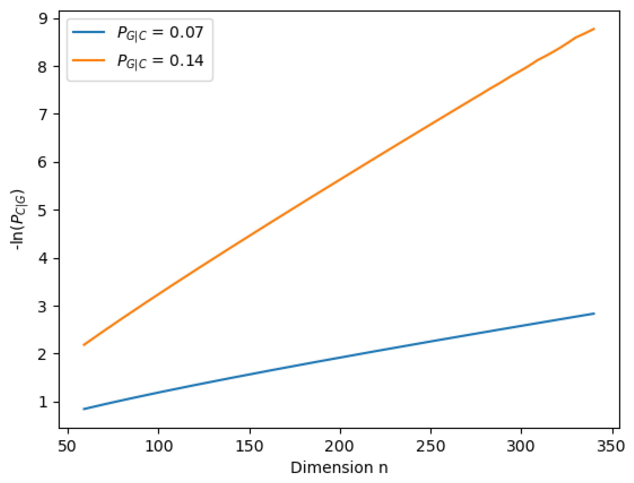
We compute the performance of the LRT defined in Equation (1) by evaluating the different quantities studied in Theorems 1 and Equation (2). For the results presented hereafter, we use and dimension . Figure A1 depicts the behavior of the Bayesian probability of error function of n for different values of the a priori. Figure A1 shows a rather fast convergence of the approximate expression presented in Theorem 1 to the numerically evaluated (3). In Figure A2, we consider Case 1 in Theorem 2 and plot the numerically evaluated error of the second kind versus n, in addition to the approximate expression for different values of . Again, the fast convergence of the approximation is observed. Finally, we depict in Figure A3 as a function of n. A linear behavior is noticed, as predicted by the result of Case 2 in Theorem 2.
Figure A1.
vs. n for . Solid line: numerical computations. Dashed line: approximate expression.
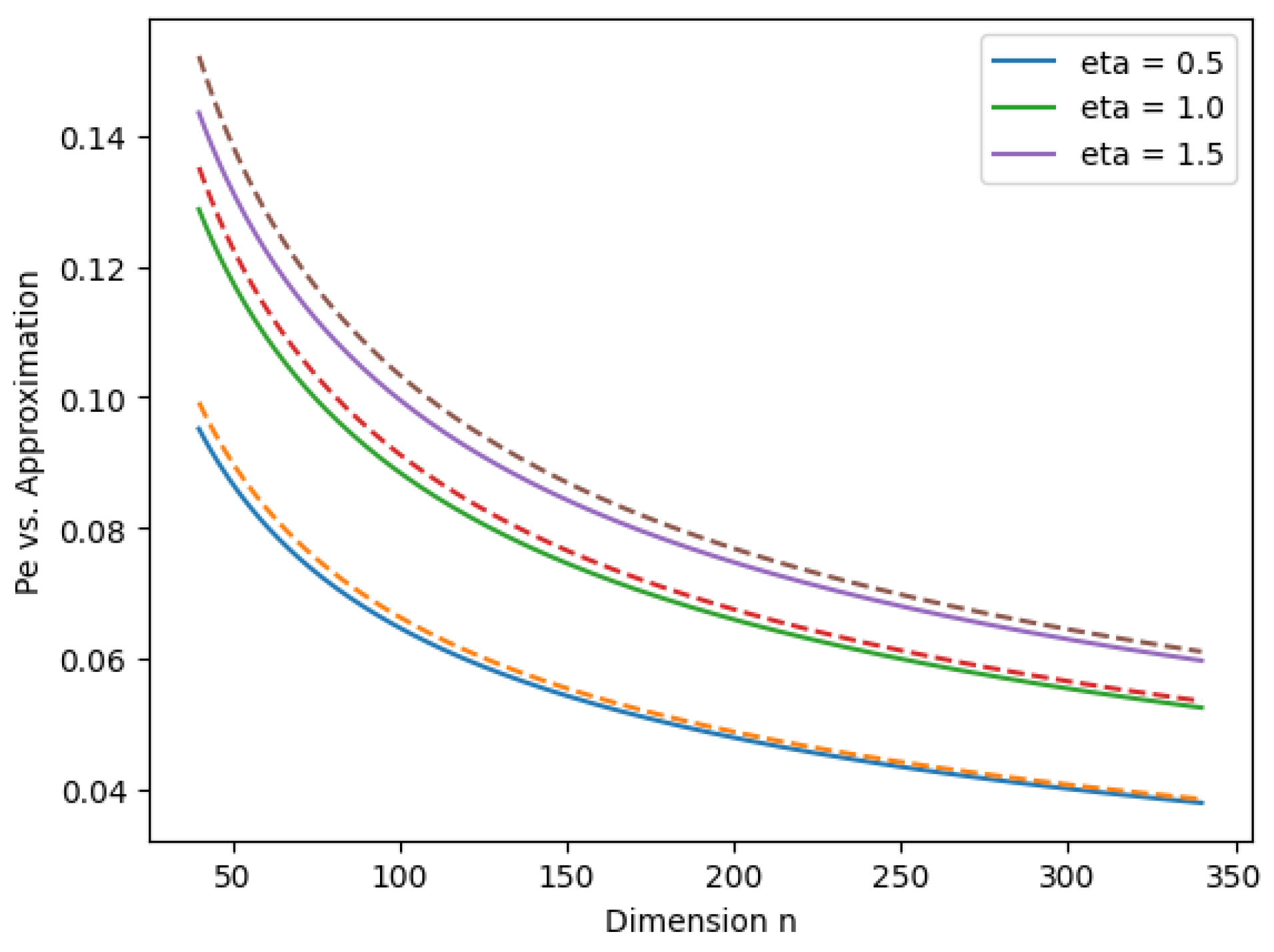
Figure A2.
vs. n for . Solid line: numerical computations. Dashed line: approximate expression.
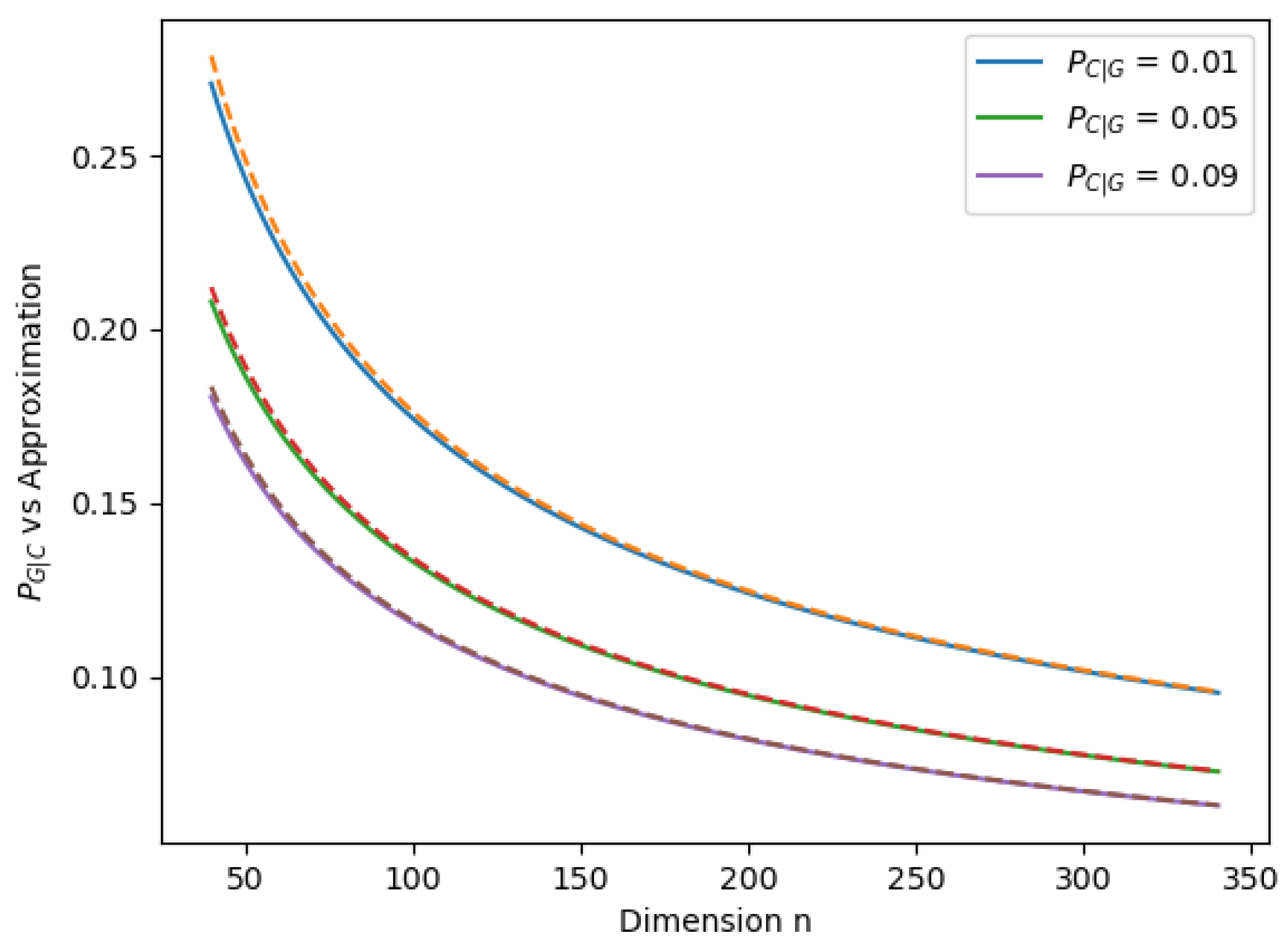
Figure A3.
vs. n for .
References
- Cover, T.M.; Thomas, J.A. Elements of Information Theory, 2nd ed.; John Wiley & Sons: Hoboken, NJ, USA, 2006. [Google Scholar]
- Tusnády, G. On asymptotically optimal tests. Ann. Stat. 1977, 5, 385–393. [Google Scholar] [CrossRef] [Scilit]
- Csiszar, I. The method of types [information theory]. IEEE Trans. Inf. Theory 1998, 44, 2505–2523. [Google Scholar] [CrossRef] [Scilit]
- Gnedenko, B.V.; Kolmogorov, A.N. Limit Distributions for Sums of Independent Random Variables; Addison-Wesley Publishing Company: Reading, MA, USA, 1968. [Google Scholar]
- Nassar, M.; Gulati, K.; Sujeeth, A.; Aghasadeghi, N.; Evans, B.; Tinsley, K. Mitigating near-field interference in laptop embedded wireless transceivers. In Proceedings of the IEEE International Conference on Acoustics, Speech and Signal Processing, Las Vegas, NV, USA, 30 March–4 April 2008; pp. 1405–1408. [Google Scholar] [CrossRef] [Scilit]
- Win, M.; Pinto, P.; Shepp, L. A mathematical theory of network interference and its applications. Proc. IEEE 2009, 97, 205–230. [Google Scholar] [CrossRef] [Scilit]
- Tsihrintzis, G.; Tsakalides, P.; Nikias, C. Signal detection in severely heavy-tailed radar clutter. In Proceedings of the Conference Record of The Twenty-Ninth Asilomar Conference on Signals, Systems and Computers, Pacific Grove, CA, USA, 30 October–1 November 1995; Volume 2, pp. 865–869. [Google Scholar] [CrossRef] [Scilit]
- Crovella, M.E.; Taqqu, M.S.; Bestavros, A. Heavy-tailed probability distributions in the World Wide Web. Pract. Guide Heavy Tails 1998, 1, 3–26. [Google Scholar]
- Nolan, J.P. Multivariate elliptically contoured stable distributions: Theory and estimation. Comput. Stat. 2013, 28, 2067–2089. [Google Scholar] [CrossRef] [Scilit]
- Nolan, J.P. Maximum Likelihood Estimation and Diagnostics for Stable Distributions. In Lévy Processes: Theory and Applications; Birkhäuser Boston: Boston, MA, USA, 2001; pp. 379–400. [Google Scholar] [CrossRef] [Scilit]
- Kuruoglu, E.; Zerubia, J. Modeling SAR images with a generalization of the Rayleigh distribution. IEEE Trans. Image Process. 2004, 13, 527–533. [Google Scholar] [CrossRef] [Scilit] [PubMed]
- Rahimi, A.; Recht, B. Random Features for Large-Scale Kernel Machines. In Proceedings of the 20th International Conference on Neural Information Processing Systems (NIPS’07), Vancouver, BC, Canada, 3–6 December 2007; Curran Associates Inc.: Red Hook, NY, USA, 2007; pp. 1177–1184. [Google Scholar]
- Mei, S.; Montanari, A. The Generalization Error of Random Features Regression: Precise Asymptotics and the Double Descent Curve. Commun. Pure Appl. Math. 2019, 75, 667–766. [Google Scholar] [CrossRef] [Scilit]
- Gerace, F.; Loureiro, B.; Krzakala, F.; Mézard, M.; Zdeborová, L. Generalisation error in learning with random features and the hidden manifold model. J. Stat. Mech. Theory Exp. 2021, 2021, 124013. [Google Scholar] [CrossRef] [Scilit]
- Adomaityte, U.; Sicuro, G.; Vivo, P. Classification of Heavy-tailed Features in High Dimensions: A Superstatistical Approach. In Proceedings of the 37th International Conference on Neural Information Processing Systems (NIPS ’23), New Orleans, LA, USA, 10–16 December 2023; Curran Associates Inc.: Red Hook, NY, USA, 2023; pp. 43880–43893. [Google Scholar]
- Beck, C. Superstatistics: Theory and Applications. Contin. Mech. Thermodyn. 2003, 16, 293–304. [Google Scholar] [CrossRef] [Scilit]
- Wainwright, M.J.; Simoncelli, E. Scale Mixtures of Gaussians and the Statistics of Natural Images. In Proceedings of the Advances in Neural Information Processing Systems, Denver, CO, USA, 29 November–4 December 1999; Solla, S., Leen, T., Müller, K., Eds.; MIT Press: Cambridge, MA, USA, 1999; Volume 12. [Google Scholar]
- Adomaityte, U.; Defilippis, L.; Loureiro, B.; Sicuro, G. High-dimensional robust regression under heavy-tailed data: Asymptotics and Universality. arXiv 2023, arXiv:2309.16476. [Google Scholar] [CrossRef] [Scilit]
- Samoradnitsky, G.; Taqqu, M.S. Stable Non-Gaussian Random Processes: Stochastic Models with Infinite Variance; Chapman and Hall: New York, NY, USA, 1994. [Google Scholar]
- Corless, R.M.; Gonnet, G.H.; Hare, D.E.G.; Jeffrey, D.J.; Knuth, D.E. On the LambertW function. Adv. Comput. Math. 1996, 5, 329–359. [Google Scholar] [CrossRef] [Scilit]
- Butler, R.W. Saddlepoint Approximations with Applications; Cambridge Series in Statistical and Probabilistic Mathematics; Cambridge University Press: Cambridge, UK, 2007. [Google Scholar] [CrossRef] [Scilit]
- Borjesson, P.; Sundberg, C.E. Simple Approximations of the Error Function Q(x) for Communications Applications. IEEE Trans. Commun. 1979, 27, 639–643. [Google Scholar] [CrossRef] [Scilit]
- Hisakado, M.; Kitsukawa, K.; Mori, S. Correlated Binomial Models and Correlation Structures. J. Phys. Gen. Phys. 2006, 39, 15365. [Google Scholar] [CrossRef] [Scilit]
- Nicola, V.; Goyal, A. Modeling of correlated failures and community error recovery in multiversion software. IEEE Trans. Softw. Eng. 1990, 16, 350–359. [Google Scholar] [CrossRef] [Scilit]
- Spencer, J.H.; Florescu, L. Asymptopia; American Mathematical Society: Providence, RI, USA, 2014. [Google Scholar]
Disclaimer/Publisher’s Note: The statements, opinions and data contained in all publications are solely those of the individual author(s) and contributor(s) and not of MDPI and/or the editor(s). MDPI and/or the editor(s) disclaim responsibility for any injury to people or property resulting from any ideas, methods, instructions or products referred to in the content. |
© 2024 by the authors. Licensee MDPI, Basel, Switzerland. This article is an open access article distributed under the terms and conditions of the Creative Commons Attribution (CC BY) license (https://creativecommons.org/licenses/by/4.0/).