Coal Quality Analysis Based on Laser-Induced Breakdown Spectroscopy

Abstract

The study presents a novel approach that integrates laser-induced breakdown spectroscopy (LIBS) data with machine learning algorithms for the rapid evaluation of coal quality. The developed framework enables the determination of three critical parameters: Ash Content (A_ad), Carbon Content (C_d), Sulfur Content (S_tad). The experimental implementation utilized an optimized dataset to construct and evaluate the predictive model. The LIBS prototype system enables spectral data acquisition under controlled experimental conditions. Data preprocessing is carried out by systematically removing background interference and substrate effects using adaptive filtering techniques. Characteristic emission peaks corresponding to target elements are identified through multivariate analysis, and Partial Least Squares Regression (PLSR) serves as the core algorithm for analysis. Systematic iterative optimization of multivariate preprocessing parameters and adaptive peak selection strategies yields substantial improvements in both predictive accuracy and computational efficiency, with determination coefficients (R² > 0.90) demonstrated for all target analytes. This enhanced accuracy validates the viability of LIBS as a robust alternative to conventional analytical methods for coal composition analysis. The LIBS demonstrates substantial advantages in coal quality assessment, thereby enhancing the overall efficiency of both coal extraction and quality evaluation processes.

1. Introduction

Since the First Industrial Revolution, coal has served as an indispensable energy source and continues to occupy a crucial position in the global energy structure. Although the development of new energy alternatives has influenced coal consumption, its central role in the energy mix remains irreplaceable. Therefore, rapid and efficient methods for coal quality assessment have become a pressing need.

LIBS is a technique that focuses high-energy pulsed lasers onto the surface of a sample. The laser ablation generates high-temperature plasma, causing atoms and ions in the sample to be heated and ionized, leading to the formation of highly excited states and the creation of micro-scale ablation pits on the surface. As these excited species relax from higher to lower energy levels, they emit photons. Because each element has a distinct atomic structure, the resulting emission spectra contain distinct spectral lines characteristic of the elements present. By collecting and analyzing the plasma spectra, it is theoretically possible to determine the elemental composition of a sample.

With advances in artificial intelligence, laser, and optical technologies, LIBS has been applied across diverse fields. In the biomedical domain, Rania M Abdelazeem et al. effectively distinguished normal serum samples from inflammatory serum samples by depositing serum samples onto ashless filter paper and inducing plasma emission through exposure to a high-power Nd:YAG laser source, followed by spectral information collection and analysis [1]. David Pokrajac et al. employed principal component analysis as a dimensionality reduction method (K-nearest neighbors, classification and regression trees, neural networks, support vector machines, adaptive local hyperplanes, and linear discriminant classification) to achieve high-precision automated classification of complex protein samples from LIBS data [2]. Jonathan Diedrich et al. employed LIBS to identify pathogenic E. coli strains, experimentally demonstrating the technique’s potential for distinguishing pathogenic strains from common environmental strains [3]. Additionally, LIBS enables quantitative analysis of trace metal accumulation in teeth [4]. The integration of LIBS with machine learning for diagnosing and staging multiple myeloma offers a rapid, minimally invasive, cost-effective, and robust approach for human malignant tumor diagnosis and staging [5]. In environmental science, Melinda Darby-Dale et al. compared LIBS with PLS regression combined with lasso modeling for analyzing geological samples [6]. Alexander Potnov et al. applied LIBS to characterize emissions from nitroaromatic compounds (NC) and polycyclic aromatic hydrocarbons (PAH) in ambient air samples. Their study demonstrated the potential to distinguish one chemical category from another, and under optimal conditions, even identify specific compounds using LIBS [7]. Bruno Bousquet et al. developed a mobile LIBS-based system specifically for in situ analysis of contaminated soils, describing the creation of a portable LIBS system dedicated to in situ analysis of heavy metal-contaminated soils [8]. In deep space exploration, LIBS technology can analyze mineral elements on unknown planets. For instance, LIBS has been employed for the analysis and study of Martian elements and minerals [9,10,11]. Due to its non-destructive nature, LIBS is also utilized in archaeology, cultural heritage identification, and conservation [12,13]. LIBS technology offers novel physical approaches for chemical element analysis [14,15,16,17]. LIBS has been successfully applied for detecting trace elements such as chromium, lead, and copper in soil [18,19,20,21]. The feasibility of using LIBS to detect sulfur, ash content, and carbon levels in coal has also been successfully validated [22].

This study proposes a novel approach for coal quality detection that integrates LIBS with machine learning. This approach is operable, fast, safe, environmentally friendly, and highly flexible. It utilizes plasma spectra excited by high-energy lasers to determine the elements present in coal [23,24]. As a non-destructive technique, it ensures repeatability while significantly reducing experimental costs. In recent years, with the advancement of artificial intelligence, the integration of machine learning algorithms with spectral data has substantially enhanced the intelligence and accuracy of material analysis in engineering applications [25,26,27].

Significant variations in sulfur content (S_tad), ash content (A_ad), and carbon content (C_d) among different coal types lead to corresponding differences in combustion efficiency and pollutant emissions. High sulfur content increases the risk of low-temperature corrosion and spontaneous combustion of coal dust, while also directly determining the amount of sulfur dioxide (SO₂) released during combustion. Accurate sulfur detection, therefore, enables more effective control of the combustion process to mitigate sulfur oxide emissions. Ash is a detrimental component of coal, as it adversely affects both utilization and combustion efficiency [28]. When coal is used as a power fuel, the higher the ash content, the lower the content of combustible substances in coal. Thus, the ash content is related to multiple factors, which can be roughly classified into three categories: (1) primary minerals, i.e., the inorganic matters inherent in the plants forming coal; (2) secondary minerals, i.e., the minerals entering the coal seam during the coal formation process; (3) extraneous minerals, i.e., rock and gangue debris mixed in during coal mining. The components include, but are not limited to, SiO₂, Al₂O₃, Fe₂O₃, CaO, MgO, SO₃, K₂O, Na₂O, etc., and may also contain trace heavy metals and harmful elements (e.g., As, Hg, Pb, etc.). Combustion of these components releases toxic gases (e.g., arsenic trioxide, mercury vapor, etc.), polluting the environment [29,30]. Additionally, the carbon content also affects the ash proportion: the higher the carbon content, the lower the ash content after complete combustion of coal. Ash content strongly influences coal combustion efficiency. Coals with higher ash content are more difficult to ignite, burn less stably, and experience greater heat loss due to incomplete combustion. In industrial applications, the excessive ash content also impacts the service life of furnace chambers. Conversely, higher carbon content enhances combustibility, reduces combustion losses, and releases greater heat, thereby improving overall combustion efficiency [31].

Sulfur, ash, and carbon contents are key indicators of coal quality [32]. Traditional methods for determining sulfur content include gravimetric techniques (e.g., Eschka method) and coulometric titration. For instance, the gravimetric method involves mixing the coal sample with Eschka reagent and igniting it at 850 °C, converting sulfur into sulfate, which precipitates as barium sulfate. The sulfur content is then calculated by weighing the precipitate, a process that typically requires 4–6 h. Similarly, ash content is traditionally measured by igniting a coal sample in a muffle furnace at 550 °C until a constant weight is achieved, with the remaining residue quantified as ash. Carbon content is commonly determined using the two-stage furnace method, in which the furnace temperatures are set to 850 °C and 500 °C. Following pyrolysis with silver permanganate, interfering substances such as chlorine and nitrogen are removed, and the carbon content is calculated from the amount of carbon dioxide produced. All of these traditional methods for determining sulfur, ash, and carbon contents are based on combustion processes, which are time-consuming, labor-intensive, and destructive, making them unsuitable for the real-time and rapid analysis required by the modern coal industry applications.

In this study, a novel method is developed for rapid and online analysis of key quality indicators in coal—namely, ash, carbon, and sulfur contents—based on LIBS [33,34]. Conventional coal quality assessment methods are typically laboratory-dependent, time-consuming, and labor-intensive, making them inadequate for meeting the modern coal industry’s demand for real-time quality monitoring and efficient sorting. In contrast, LIBS offers remarkable advantages, including minimal sample preparation, high analysis speed, multi-element detection capability, and strong potential for online applications, rendering it an attractive candidate technique for this purpose. However, the intrinsic complexity and heterogeneity of coal introduce challenges such as spectral interference, matrix effects, and measurement instability, which hinder the analytical performance of LIBS in coal analysis. Therefore, the primary objective of this work is to establish a robust analytical model through algorithm optimization, thereby significantly enhancing the accuracy and reliability of ash, carbon, and sulfur content determination in coal. The anticipated outcomes are expected to provide powerful technical support for rapid coal quality evaluation, combustion efficiency optimization, and emission control, thus contributing to the advancement of clean and efficient coal utilization.

2. Experimental Setup

The principle of LIBS is illustrated in Figure 1.

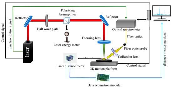
Figure 1. Schematic diagram of a typical LIBS system.

The core of the LIBS system employed in this experiment comprises a Beamtech Nd:YAG laser operating at a wavelength of 1064 nm, with a pulse width of 8 ns and a maximum energy of 200 mJ. The laser generates a pulsed beam whose output energy is modulated through a combination of a half-wave plate and a polarizing beam splitter. Utilizing two mirrors and a focusing lens (f = 150 mm, ϕ = 25.4 mm) to focus the laser beam onto the surface of the sample under test, inducing plasma generation. The resulting plasma luminescence signal is captured by another collection lens with a focal length of 15 mm and transmitted through a multimode fiber to the AVANTES fiber spectrometer (spectral range 181–769 nm, resolution approximately 0.15 nm). The laser distance meter (Figure 1), combined with a data acquisition card, provides the focal length information for the sample to adjust the focusing position of the pulsed laser after the lens. The Z-axis of the three-dimensional translation stage received the feedback signal from a laser distance meter to ensure precise focusing. During measurements, coal samples were placed on the translation stage for cyclic scanning. Under computer control, the X- and Y-axes of the stage guided the laser to irradiate the sample in a 5 × 5 matrix. A fixed number of laser pulses was applied at each sampling point, and the averaged spectrum of the coal sample was obtained by accumulating repeated shots. Simultaneously with laser emission, the internal clock synchronously outputs pulses as a timing reference. This pulse output triggers the spectrometer’s time-delayed acquisition, achieving precise synchronization between the laser pulse and spectral collection.

Based on the above analysis, this study proposes a direct measurement method utilizing LIBS. We hypothesize that LIBS technology can directly and simultaneously detect the characteristic spectral signal intensities of carbon and sulfur in coal. Furthermore, since ash is a mixture of various elements and non-combustible substances in coal, we hypothesize that a correlation can be established between ash content and the various elements present in coal. Based on this, we establish a predictive model for ash content to enable accurate prediction. To validate these hypotheses, this experiment will collect spectral signals from coal using LIBS. A partial least squares regression algorithm will be employed to establish regression models for carbon, sulfur, and ash content, enabling analysis of these components.

3. Materials and Methods

3.1. Sample Preparation

The samples used in this study were obtained from the reserve stock of a thermal power plant, with a total of 83 true value samples. The true values of sulfur, ash content, and carbon content from these samples were used as the reference data for modeling. Table 1 presents the true values of the samples used for modeling.

Table 1. True values of sulfur, ash, and carbon contents in the coal samples.

No.	Aad (wt.%)	Cd (mg/kg)	Stad (mg/kg)	No.	Aad (wt.%)	Cd (mg/kg)	Stad (mg/kg)
1	25.62	62.67	0.79	43	25.63	62.47	0.64
2	25.49	62.42	0.70	44	25.20	61.98	0.60
3	25.44	64.30	0.86	45	27.40	60.24	0.63
4	23.94	65.20	0.62	46	29.66	59.78	1.09
5	26.07	63.95	0.70	47	28.66	60.72	1.02
6	27.27	63.71	0.71	48	26.64	61.59	1.06
7	25.92	62.79	0.66	49	24.82	64.94	0.62
8	27.64	62.36	0.72	50	25.92	63.67	0.90
9	30.04	59.27	0.69	51	25.74	63.34	0.86
10	28.71	61.30	0.70	52	29.72	60.36	0.86
11	29.19	60.74	0.53	53	27.02	62.51	0.84
12	32.64	62.92	0.86	54	26.76	62.13	0.94
13	29.83	64.06	0.65	55	29.66	59.09	0.78
14	29.34	59.29	0.70	56	30.41	58.78	0.82
15	33.48	55.37	0.66	57	32.68	56.85	0.98
16	28.40	61.32	0.82	58	33.86	56.60	1.03
17	30.64	57.61	0.60	59	31.51	57.63	0.82
18	27.00	62.75	0.75	60	32.09	56.72	0.90
19	24.82	63.25	0.74	61	29.71	58.60	1.10
20	27.22	62.29	0.92	62	29.72	58.63	1.00
21	28.88	60.92	0.67	63	27.36	61.60	0.74
22	29.17	60.09	0.58	64	24.23	62.53	1.12
23	29.79	62.13	0.66	65	27.77	61.63	0.74
24	27.14	62.58	0.64	66	31.43	58.10	1.10
25	28.88	60.31	0.62	67	29.97	60.00	0.94
26	29.44	60.94	0.62	68	28.85	60.55	0.72
27	29.14	59.37	0.72	69	32.02	58.46	1.12
28	27.86	62.41	0.73	70	30.78	61.56	0.98
29	27.02	63.45	0.59	71	29.86	60.39	0.96
30	25.52	65.03	0.64	72	26.90	62.42	0.84
31	26.20	63.60	0.50	73	27.84	61.29	1.02
32	29.16	60.89	0.70	74	27.60	63.14	0.87
33	24.32	63.87	0.60	75	30.62	58.60	0.98
34	23.10	66.04	0.74	76	28.92	60.20	0.88
35	27.36	63.40	0.52	77	27.36	63.08	0.66
36	22.92	64.37	0.58	78	29.77	58.93	0.88
37	21.26	64.59	0.63	79	33.10	56.42	1.03
38	21.20	65.73	0.54	80	26.10	62.53	0.78
39	23.80	64.41	0.52	81	28.21	61.51	0.86
40	24.29	63.02	0.58	82	25.90	62.74	0.82
41	23.54	63.89	0.58	83	29.50	58.24	0.84
42	23.64	62.17	0.58

The feasibility of LIBS-based online coal quality analysis has been well established, and equipment for various measurement methods, including coal block analysis, coal powder analysis, and pellet sample preparation, has been developed [35,36]. Currently, pellet sample preparation remains the most suitable approach for LIBS-based online coal quality assessment. In this work, since it is necessary to focus a high-energy pulsed laser onto the sample surface, standard samples with uniform heights were required. A total of 83 true-value samples, each containing the same mass of coal powder, were placed into molds and pressed under identical pressure to form standard pellets. These samples exhibit uniform height, eliminating the need for focus adjustments when changing samples. This uniformity ensures experimental rigor by controlling sample height as a consistent variable. Figure 2 illustrates the standard sample prepared by compressing the powder into a solid pellet using molds.

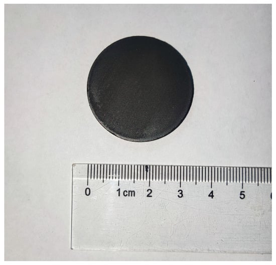
Figure 2. Standard coal sample prepared for LIBS analysis.

The prepared standard samples were placed into the LIBS prototype, and a 5 × 5 × 5 point pattern was set (each sample consisted of five rows and five columns, with each point measured five times); the distance between each point is 3 mm. In this experiment, each sample underwent the sample preparation process shown in the figure above. A total of 83 samples were involved, and LIBS spectral data were collected from 83 standard samples. Since the ablation craters are on the micron scale, the depth of the ablation craters is negligible.

3.2. Spectral Preprocessing

The spectra obtained directly from the LIBS prototype are referred to as raw spectra. Due to the presence of noise in these spectra, they cannot be used directly for modeling. Prior to model development, the raw spectra must be preprocessed to minimize interfering factors and ensure the accuracy and reliability of the predictive model.

3.2.1. Background Spectrum Removal

Before standardizing and normalizing the raw spectra, it is necessary to remove background light from data affected by other light sources during collection. The background correction process can be expressed by the following equation:

$$I=I_{raw}-I_{background}$$

(1)

Here, $I$ represents the background-corrected spectral intensity, $I_{raw}$ is the measured spectral data affected by background light, and $I_{background}$ is the background spectral data. Since no additional light sources are present in the sample chamber of the LIBS prototype used in this experiment, the background spectral data is set to zero, $I_{background}=0$. Therefore, the background-corrected data is equivalent to the collected raw spectral data, i.e., $I=I_{raw}$.

3.2.2. Data Cleaning

The coal spectral data collected in this experiment are stored as one-dimensional matrices of size 1 × 4094, with 125 spectra acquired for each sample. In the first step, the mean spectrum is calculated by averaging the 125 spectra column-wise at each wavelength, yielding an average spectral intensity vector of size 1 × 4094. In the second step, the deviation of each individual spectrum from the mean spectrum is computed, followed by the calculation of the sum of squares of these deviations. In the third step, spectra that exceed a threshold are excluded, where the threshold is defined as 1.1 times the sum of squares. The formulas for these steps are expressed as follows:

$${avg}_j={\displaystyle \frac{1}{125}}\sum _{i=1}^{125}{I}_{i,j}$$

(2)

here, $i$ and $j$ represent the measurement number and the number of specific wavelengths, respectively. The final result is

$$V=\left[{avg}_1,{avg}_2,{avg}_3\cdots {avg}_{4094}\right]$$

(3)

where $V$ represents the calculated average value vector.

$$A_i=\sum _{j=1}^{4094}{(I_{i,j}-{avj}_j)}^2$$

(4)

In the above equation, $A_i$ represents the sum of squares of the difference between the $i$-th measurement and the average value.

$$C_{threshold}=1.1\times \left({\displaystyle \frac{1}{150}}\sum _{i=1}^{150}{A}_i\right)$$

(5)

where $C_{threshold}$ represents the threshold value required for the selection process.

If the $i$-th data point in $A_i$ exceeds $C_{threshold}$, the corresponding $i$-th row of the spectral matrix $I_{i,j}$ will be excluded.

3.2.3. Normalized De-Basing

Due to significant variations in the characteristic spectral line intensities across different wavelengths corresponding to various elements within the full LIBS spectrum, the disparate scales (dimensionality) of the data adversely impact model performance. To enhance computational efficiency and eliminate factors detrimental to model iterative calculations, data normalization is required. The normalization formula is as follows:

$$I_{normalized}={\displaystyle \frac{I-I_{min}}{I_{max}-I_{min}}}$$

(6)

where $I_{normalized}$ represents the normalized spectral intensity, $I$ is the spectral intensity value after data cleaning, $I_{min}$ is the minimum spectral intensity within each dataset, and $I_{max}$ is the maximum spectral intensity within each dataset.

Low-frequency signals, such as noise generated by the instrument, environmental light scattering, and sample matrix effects (e.g., fluorescence, scattering), are often present in the baseline of spectral data. These signals can obscure the characteristic peaks of the target analytes (e.g., elemental spectral lines or molecular absorption peaks) and overwhelm the weak peaks of trace components. In the experiment, baseline removal is employed to improve the signal-to-noise ratio, making the target peaks more prominent and revealing weak peaks that were previously submerged, thus facilitating the identification of key elemental features. Baseline removal in this study is performed using a sliding window method. This approach involves sequentially extracting each specific wavelength within the wavelength range of the spectrometer, from small to large. For each specific wavelength, a left and right window range is set, and the minimum spectral intensity within that range is identified. The spectral intensities corresponding to all individual wavelengths within the window range are then subtracted by this minimum value to achieve baseline removal. The changes in the spectral data before and after baseline removal are shown in Figure 3.

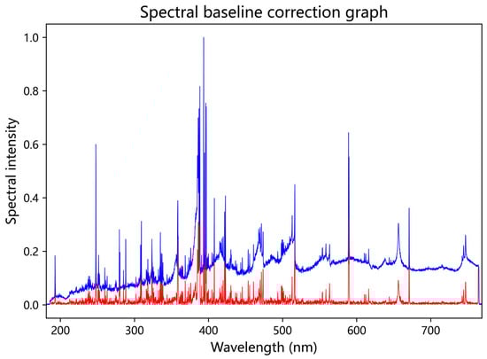
Figure 3. Comparison of before and after basal correction. The blue curve represents the unprocessed spectrum, while the red curve shows the LIBS spectrum after baseline correction.

3.3. Partial Least Squares Regression (PLSR)

PLSR is a statistical multivariate data analysis method that is particularly effective in situations where multicollinearity exists between the dependent and independent variables. It excels in handling high-dimensional data and small sample problems. The core of PLSR is a black-box algorithm based on latent linear relationships for prediction. It establishes a linear relationship model between the independent and dependent variables through both dimensionality reduction and regression methods. Unlike traditional multiple linear regression, PLSR does not directly fit the original variables but instead extracts a set of new composite variables called “latent variables,” which maximize the covariance between the independent and dependent variables, thus avoiding the instability of the model caused by multicollinearity. First introduced in 1983 by S. Wold, C. Albano, and others, PLSR has rapidly developed in theory, methodology, and applications over recent decades [37]. As a multivariate linear regression analysis technique, it has been widely used in fields such as chemistry, environmental science, biomedicine, and finance [38]. Relevant literature indicates that PLSR combined with hyperspectral data is effective for estimating soil organic matter content. This evidence demonstrates that integrating PLSR with spectral data is a viable analytical approach.

3.4. Evaluation Parameters

The evaluation parameters for PLSR include the coefficient of determination (R²), root mean square error of the test set (RMSEP), and root mean square error of cross-validation (RMSECV), which are defined as follows:

$$R^2=1-{\displaystyle \frac{\sum _i^n{(y_i-{\widehat{y}}_i)}^2}{\sum _i^n{(y_i-{\overline{y}}_i)}^2}}$$

(7)

$$RMSEP=\sqrt{{\displaystyle \frac{\sum _i^m{(y_i-{\widehat{y}}_i)}^2}{m}}}$$

(8)

$$RMSECV=\sqrt{{\displaystyle \frac{\sum _i^n{(y_i-{\widehat{y}}_i)}^2}{n-1}}}$$

(9)

where $y_i$ and ${\widehat{y}}_i$ represent the reference values and predicted values, respectively, ${\overline{y}}_i$ is the mean reference value, $m$ denotes the number of coal samples in the test set, and $n$ represents the number of coal samples in the training set.

4. Results

In this experiment, 67 processed full-spectrum datasets are used as the training set for the PLSR model, and 16 datasets are used as the test set. According to baseline correction theory, an excessively small window value may remove useful spectral information. Based on empirical evaluation, a window value of 16 is selected. The number of latent variables (n_components) is a core parameter of the PLSR model, and the size of latent variables directly affects the complexity, prediction accuracy, and generalization ability of the established model. The core goal of the PLSR experiment is to achieve the maximum prediction accuracy with the fewest components, and cross-validation was preferentially adopted to select the optimal number of latent variables.

Figure 4 illustrates the determination of the optimal number of latent variables for the PLSR model of ash content in coal samples, obtained by comparing the root mean square errors (RMSE) of cross-validation with those of the training set. The resulting optimal latent variable number for the ash model was 5. Similarly, Figure 5 and Figure 6 present the selection of latent variables for the PLSR models of sulfur and carbon in coal samples, respectively. The optimal numbers of latent variables determined for sulfur and carbon were 6 and 5. Figure 4, Figure 5 and Figure 6 show the determination of the optimal number of latent variables for ash, sulfur, and carbon prediction, with the results summarized in Table 2. Based on a comprehensive evaluation, a latent variable count of five (L = 5) is ultimately selected for all models.

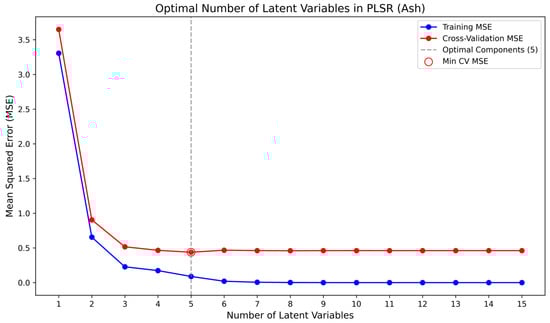
Figure 4. Optimal selection diagram of latent variables for ash content.

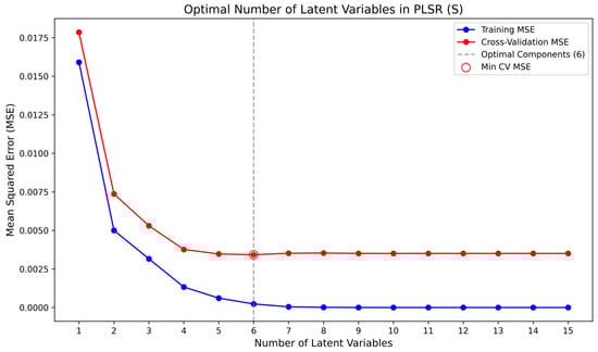
Figure 5. Optimal Selection Diagram of Latent Variables for Sulfur Component.

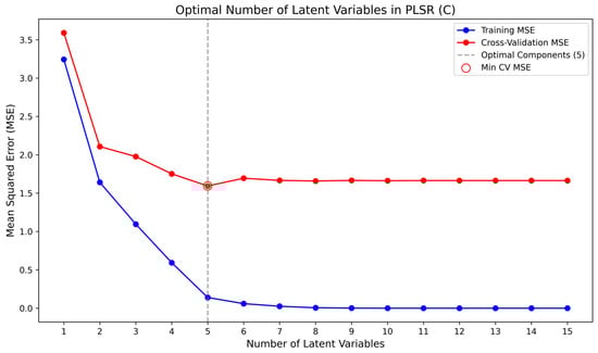
Figure 6. Optimal Selection Diagram of Latent Variables for Carbon Component.

Table 2. Optimal Selection of Latent Variables in PLSR Model.

Element	n_Components
Aad	5
Cd	6
Stad	5

Following the selection of relevant parameters, models were constructed to predict the ash content, sulfur content, and carbon content in coal samples. To enhance model generalizability, the actual measured values of ash content, sulfur content, and spectral data were sorted in ascending order. A subset of spectral data points was then systematically sampled from this sorted sequence to form the test set. This subset was selected to approximately cover the low, medium, and high ranges of the actual measurement values, ensuring it broadly represents the distribution of the entire dataset. The remaining data constituted the training set. The performance plots generated by the resulting models are presented below (Figure 7, Figure 8 and Figure 9).

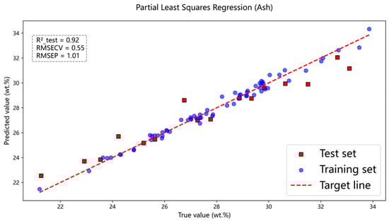
Figure 7. Full-spectrum modeling effect of ash content.

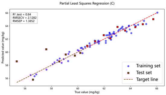
Figure 8. Spectral modeling effect of carbon content composition.

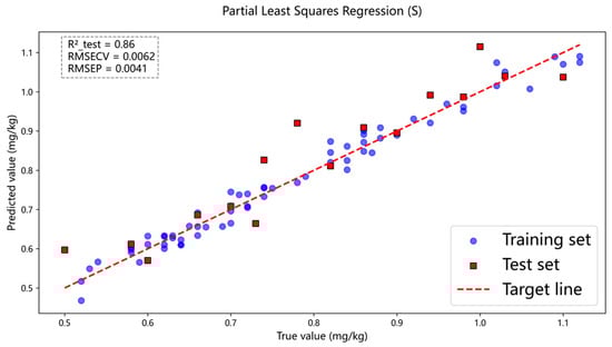
Figure 9. Spectral modeling effect diagram of sulfur content.

Figure 7 presents the prediction results of ash content in coal samples using the full-spectrum data, where the PLSR model achieved $R^2=0.92$, $RMSECV=0.55$ and $RMSEP=1.01$. Figure 8 and Figure 9 show the prediction results for carbon and sulfur, respectively. For carbon, the PLSR model yielded $R^2=0.84$, $RMSECV=2.1282$ and $RMSEP=1.3852$, and for sulfur, the corresponding values were $R^2=0.86$, $RMSECV=0.0062$ and $RMSEP=0.0041$. Here, $R^2$ denotes the coefficient of determination for the test set, while $RMSECV$ and $RMSEP$ represent the root mean square error for cross-validation and the test set, respectively. In comparison, the prediction accuracy for carbon in coal was relatively lower. This may be attributed to the fact that carbon constitutes the most abundant element in coal, resulting in the strongest self-absorption effect. Due to the influence of this self-absorption effect, analyzing the carbon spectrum becomes challenging.

4.1. Selection of Spectral Peaks in LIBS Data

To further enhance model performance, this study builds upon the fundamental principles of LIBS. Within the full-spectrum data, peak identification algorithms are employed to isolate and retain exclusively the peak data, discarding all non-peak information. As distinct elements possess unique atomic structures, their corresponding excited ionic spectra exhibit characteristic differences. These elemental fingerprints are preserved within the retained peak data. However, potential instrumental limitations of the LIBS prototype, including spectrometer wavelength shifts, nonlinear grating dispersion, detector pixel misalignment, and insufficient spectral resolution, may cause the acquired spectral peaks to deviate from the reference wavelengths reported in the NIST database. Consequently, the entire set of peak data is directly utilized for modeling and analysis, and its effectiveness is compared with that of models constructed using the full spectrum.

Following the establishment of underlying principles, the next step involves peak detection in the spectroscopic data. In LIBS data analysis, peak finding constitutes a fundamental step in processing, underpinning the entire workflow from raw spectral interpretation to elemental quantification. This process serves as the critical bridge converting LIBS spectral data into elemental information. Models utilize characteristic peaks for both qualitative identification and analysis. The positions of identified peaks at specific wavelengths form the basis of qualitative models, while the intensity of these peaks is used to detect the content of the substances they contain. Furthermore, peak finding facilitates dimensionality reduction by eliminating a portion of non-relevant spectral data. The core objective of the peak finding algorithm is to identify local maxima (peaks) within the data sequence. The selection of peak significance is controlled by implementing a threshold filter; in this experiment, a peak intensity threshold of 0.01 was applied. Figure 10 shows the peak-finding effect diagram of the full spectral data.

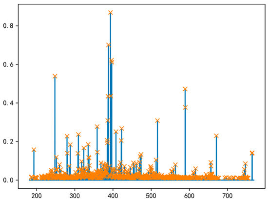
Figure 10. Peak effect diagram. Yellow markers indicate the identified spectral peaks.

Figure 11 shows the data visualization after removing non-peak data, with characteristic peak spectral lines for C and S labeled in the figure. The characteristic spectral lines for ash, sulfur, and carbon are listed in Table 3.

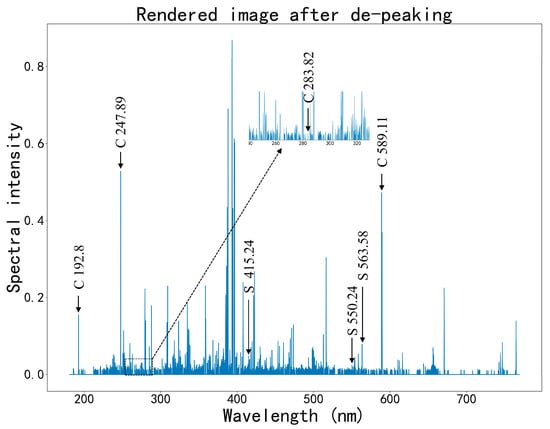
Figure 11. Effect diagram after removing non-peak data and retaining only peak data.

Table 3. Selected characteristic wavelengths for ash, sulfur, and carbon.

Element	Wavelength (nm)
Ash	K 310.46, Ti 308.37, Zn 212.52, Na 280.97, Si 288.16, Ca 393.50, Ca 396.88, Fe 344.12, Na 313.14, Mg 299.28, CN 387.17, Si 390.70, Si 251.65, N 742.59, Fe 407.90, Fe 404.68, Ti 338.47, Ti 338.92, Ti 430.75, Ti 512.98, Li 670.92, H 656.35, O 616.28, O 764.96, Fe 610.41, N 744.46, N 747.00
C	192.8, 247.89, 283.82, 589.11
S	415.24, 550.24, 563.58

4.2. Comparison of Predicted Carbon and Sulfur Contents

Models are trained using the peak-identified data, with non-peak data points set to zero. This procedure ensures that spectral regions lacking elemental fingerprint information are excluded from subsequent algorithmic computations. The selected peaks from the processed data are applied to the established model. Principal component analysis (PCA) is employed to reduce the dimensionality of the spectral peaks and to extract the principal components that contribute most significantly to the data variance. Based on the variance contribution rates of each principal component, we further implemented feature selection to eliminate peak variables with negligible explanatory impact on the model, thereby optimizing its structure and performance. The results indicate that the coefficient of determination (R²) for sulfur concentration has increased. Specifically, Figure 12 shows the sulfur concentration prediction results obtained using the peak dataset as modeling input and applying the PCA dimensionality reduction algorithm, while Figure 13 presents the corresponding prediction results for carbon concentration.

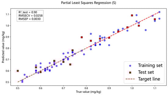
Figure 12. In the PLSR model, peak data were used as both the training and test sets, and the sulfur content prediction results were obtained by combining the PCA algorithm.

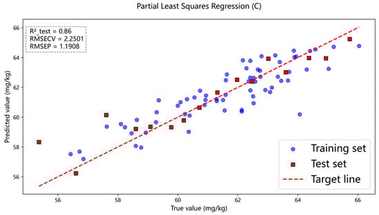
Figure 13. In the PLSR model, peak data were used as both the training and test sets, and the carbon content prediction results were obtained by combining the PCA algorithm.

As shown in Figure 12 and Figure 13, after the peak-finding operation, the coefficient of determination (R²) for sulfur increases from the original value of 0.86 to 0.90, and the coefficient of determination (R²) for carbon increases from the original value of 0.84 to 0.86. A comparative summary of these effects is presented in Table 4.

Table 4. Comparison of modeling effects before and after peak search.

Element Assessment	Stad	S After Optimization	Cd	C After Optimization
$R^2$	0.86	0.90	0.84	0.86
RMSECV	0.0062	0.00258	2.1282	2.2501
RMSEP	0.0041	0.0030	1.3852	1.1908

4.3. Handling of Ash Content

Given the numerous factors influencing ash content, manual selection of elements for ash prediction is complex and inefficient. Therefore, this experiment adopted variable recombination combined with the variable importance in the projection (VIP) index for modeling ash prediction. The VIP index is a key indicator in the PLSR model to measure the relative contribution of independent variables to explaining dependent variables.

Figure 14A shows the ash content prediction results after variable reorganization. The coefficient of determination (R²) for the test set reached 0.9058 after variable reorganization. Although this is lower than 0.92, it resolves the issue of manually selecting latent variables for each training session. Figure 14B illustrates the relative contributions of independent variables selected through the VIP index. Figure 14C depicts the optimal latent variables automatically matched by the model. This process automatically selects the best latent variables for different datasets based on changes in the RMSECV during cross-validation prior to model training. The figure indicates that the optimal latent variables are obtained when the RMSECV is 0.0998, and this approach improves the performance of the constructed model. Figure 14D demonstrates the predictive performance of the PLSR model on both the test and training datasets, visually comparing the prediction outcomes for these two sets within the model. The above model realizes the optimal selection through automated latent variable selection.

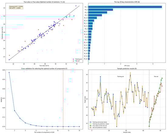
Figure 14. The final effect after reorganizing the gray-scale variables. (A). presents the ash content prediction results after variable recoding. (B). displays the relative contribution of independent variables selected via the VIP index. (C). illustrates the optimal latent variables automatically matched by the model, with the red line indicating the optimal latent variable position. (D). demonstrates the predictive performance of the PLSR model on the test and training datasets through a visual comparison of the prediction results across both datasets.

5. Conclusions

This study combines LIBS spectral data from the prototype system with PLSR modeling to predict coal composition. First, coal samples were pressed into standard coal specimens for experimental use. Data acquisition was performed on the coal samples via the LIBS system. The collected data underwent processing before being utilized for modeling. The processed full spectral data were applied to the PLSR model, yielding R² values of 0.92, 0.84, and 0.86 for ash content, carbon content, and sulfur content, respectively. Peak detection technology was employed to eliminate non-peak data. To further optimize the models, PLSR was combined with PCA, improving the R² values for sulfur and carbon content to 0.90 and 0.86, respectively, surpassing the initial results. For ash content, variable re-organization was employed to construct a prediction model yielding an R² value of 0.9058. Although slightly lower than the initial 0.92, integrating latent variable prediction algorithms into the model eliminated the need for manual latent variable input with each new data addition. Experimental results validate the feasibility of the LIBS-PLSR integrated approach for coal quality analysis, enabling real-time coal quality monitoring during mining operations. Compared to conventional methods, this technology offers higher detection efficiency and enhanced sample reusability. Furthermore, resource consumption for predicting coal composition via this model is significantly lower than that of conventional techniques. Future research should focus on model optimization to achieve optimal prediction for specific elemental components.

References

- Abdelazeem, R.M.; Salam, Z.A.; Harith, M.A. Differentiating between normal and inflammatory blood serum samples using spectrochemical analytical techniques and chemometrics. Anal. Bioanal. Chem. 2025, 417, 2133–2142. [Google Scholar] [CrossRef]
- Pokrajac, D.; Lazarevic, A.; Kecman, V.; Marcano, A.; Markushin, Y.; Vance, T.; Reljin, N.; McDaniel, S.; Melikechi, N. Automatic Classification of Laser-Induced Breakdown Spectroscopy (LIBS) Data of Protein Biomarker Solutions. Appl. Spectrosc. 2014, 68, 1067–1075. [Google Scholar] [CrossRef]
- Diedrich, J.; Rehse, S.J.; Palchaudhuri, S. Pathogenic Escherichia coli strain discrimination using laser-induced breakdown spectroscopy. J. Appl. Phys. 2007, 102, 6184. [Google Scholar] [CrossRef]
- Samek, O.; Beddows, D.C.S.; Telle, H.H.; Morris, G.W.; Liska, M.; Kaiser, J. Quantitative analysis of trace metal accumulation in teeth using Laser-Induced Breakdown Spectroscopy. Appl. Phys. A 1999, 69, S179–S182. [Google Scholar] [CrossRef]
- Chen, X.; Zhang, Y.; Li, X.; Yang, Z.; Liu, A.; Yu, X. Diagnosis and staging of multiple myeloma using serum-based laser-induced breakdown spectroscopy combined with machine learning methods. Biomed. Opt. Express 2021, 12, 3584–3596. [Google Scholar] [CrossRef] [PubMed]
- Dyar, M.D.; Carmosino, M.L.; Breves, E.A.; Ozanne, M.V.; Clegg, S.M.; Wiens, R.C. Comparison of partial least squares and lasso regression techniques as applied to laser-induced breakdown spectroscopy of geological samples. Spectrochim. Acta Part B At. Spectrosc. 2012, 70, 51–67. [Google Scholar] [CrossRef]
- Portnov, A.; Rosenwaks, S.; Bar, I. Emission following laser-induced breakdown spectroscopy of organic compounds in ambient air. Appl. Opt. 2003, 42, 2835–2842. [Google Scholar] [CrossRef]
- Bousquet, B.; Travaillé, G.; Ismaël, A.; Canioni, L.; Michel-Le Pierrès, K.; Brasseur, E.; Roy, S.; le Hecho, I.; Larregieu, M.; Tellier, S.; et al. Development of a mobile system based on laser-induced breakdown spectroscopy and dedicated to in situ analysis of polluted soils. Spectrochim. Acta Part B At. Spectrosc. 2008, 63, 1085–1090. [Google Scholar] [CrossRef]
- Arp, Z.A.; Cremers, D.A.; Wiens, R.C.; Wayne, D.M.; Sallé, B.A.; Maurice, S. Analysis of water ice and water ice/soil mixtures using laser-induced breakdown spectroscopy: Application to Mars polar exploration. Appl. Spectrosc. 2004, 58, 897–909. [Google Scholar] [CrossRef]
- Lanza, N.L.; Wiens, R.C.; Clegg, S.M.; Ollila, A.M.; Humphries, S.D.; Newsom, H.E.; Barefield, J.E. Calibrating the ChemCam laser-induced breakdown spectroscopy instrument for carbonate minerals on Mars. Appl. Opt. 2010, 49, C211–C217. [Google Scholar] [CrossRef]
- Sallé, B.; Lacour, J.L.; Vors, E.; Fichet, P.; Maurice, S.; Cremers, D.A.; Wiens, R.C. Laser-Induced Breakdown Spectroscopy for Mars surface analysis: Capabilities at stand-off distances and detection of chlorine and sulfur elements. Spectrochim. Acta Part B At. Spectrosc. 2004, 59, 1413–1422. [Google Scholar] [CrossRef]
- Tzortzakis, S.; Anglos, D.; Gray, D. Ultraviolet laser filaments for remote laser-induced breakdown spectroscopy (LIBS) analysis: Applications in cultural heritage monitoring. Opt. Lett. 2006, 31, 1139–1141. [Google Scholar] [CrossRef] [PubMed]
- Giakoumaki, A.; Melessanaki, K.; Anglos, D. Laser-induced breakdown spectroscopy (LIBS) in archaeological science-applications and prospects. Anal. Bioanal. Chem. 2007, 387, 749–760. [Google Scholar] [CrossRef] [PubMed]
- Fortes, F.J.; Ctvrtnícková, T.; Mateo, M.P.; Cabalín, L.M.; Nicolas, G.; Laserna, J.J. Spectrochemical study for the in situ detection of oil spill residues using laser-induced breakdown spectroscopy. Anal. Chim. Acta 2010, 683, 52–57. [Google Scholar] [CrossRef] [PubMed]
- Myakalwar, A.K.; Sreedhar, S.; Barman, I.; Dingari, N.C.; Rao, S.V.; Kiran, P.P.; Tewari, S.P.; Kumar, G.M. Laser-induced breakdown spectroscopy-based investigation and classification of pharmaceutical tablets using multivariate chemometric analysis. Talanta 2011, 87, 53–59. [Google Scholar] [CrossRef]
- Zhang, T.L.; Wu, S.; Tang, H.S.; Wang, K.; Duan, Y.X.; Li, H. Progress of Chemometrics in Laser-induced Breakdown Spectroscopy Analysis. Chin. J. Anal. Chem. 2015, 43, 939–948. [Google Scholar] [CrossRef]
- Parmar, D.; Srivastava, R.; Baruah, P.K. Laser induced breakdown spectroscopy: A robust technique for the detection of trace metals in water. Mater. Today 2023, 77, 234–239. [Google Scholar] [CrossRef]
- Ciucci, A.; Palleschi, V.; Rastelli, S.; Barbini, R.; Colao, F.; Fantoni, R.; Palucci, A.; Ribezzo, S.; van der Steen, H.J.L. Trace pollutants analysis in soil by a time-resolved laser-induced breakdown spectroscopy technique. Appl. Phys. B 1996, 63, 185–190. [Google Scholar] [CrossRef]
- Bousquet, B.; Sirven, J.B.; Canioni, L. Towards quantitative laser-induced breakdown spectroscopy analysis of soil sample. Spectrochim. Acta Part B At. Spectrosc. 2007, 62, 1582–1589. [Google Scholar] [CrossRef]
- Martin, M.Z.; Wullschleger, S.D.; Garten, C.T.; Palumbo, A.V. Laser-induced breakdown spectroscopy for the environmental determination of total carbon and nitrogen in soils. Appl. Opt. 2003, 42, 2072–2077. [Google Scholar] [CrossRef]
- Eppler, A.S.; Cremers, D.A.; Hickmott, D.D.; Ferris, M.J.; Koskelo, A.C. Matrix Effects in the Detection of Pb and Ba in Soils Using Laser-Induced Breakdown Spectroscopy. Appl. Spectrosc. 1996, 50, 1175–1181. [Google Scholar] [CrossRef]
- Legnaioli, S.; Campanella, B.; Pagnotta, S.; Poggialini, F.; Palleschi, V. Determination of Ash Content of coal by Laser-Induced Breakdown Spectroscopy. Spectrochim. Acta Part B At. Spectrosc. 2019, 155, 123–126. [Google Scholar] [CrossRef]
- Qian, Y.; Zhong, S.; He, Y.; Whiddon, R.; Wang, Z.H.; Cen, K.F. Effects of Laser Wavelength on Properties of Coal LIBS Spectrum. Spectrosc. Spectr. Anal. 2017, 37, 1890–1895. [Google Scholar]
- Kim, C.K.; In, J.H.; Lee, S.H.; Jeong, S. Independence of elemental intensity ratio on plasma property during laser-induced breakdown spectroscopy. Opt. Lett. 2013, 38, 3032–3035. [Google Scholar] [CrossRef]
- Agrawal, N.; Govil, H. A deep residual convolutional neural network for mineral classification. Adv. Space Res. 2023, 71, 3186–3202. [Google Scholar] [CrossRef]
- Guan, F.Y.; Liu, Y.C.; Niu, X.C.; Huang, W.H.; Li, W.; Zheng, P.C.; Zhang, D.; Xu, G.; Guo, L.B. AI-enabled universal image-spectrum fusion spectroscopy based on self-supervised plasma modeling. Adv. Photonics Nexus 2024, 3, 127–139. [Google Scholar] [CrossRef]
- Azmat, F.; Chen, Y.F.; Stocks, N. Analysis of Spectrum Occupancy Using Machine Learning Algorithms. IEEE Trans. Veh. Technol. 2016, 65, 6853–6860. [Google Scholar] [CrossRef]
- Kurose, R.; Ikeda, M.; Makino, H. Combustion characteristics of high ash coal in a pulverized coal combustion. Fuel 2001, 80, 1447–1455. [Google Scholar] [CrossRef]
- Selçuk, N.; Gogebakan, Y.; Gogebakan, Z. Partitioning behavior of trace elements during pilot-scale fluidized bed combustion of high ash content lignite. J. Hazard. Mater. 2006, 137, 1698–1703. [Google Scholar] [CrossRef]
- Lee, M.G.; Yi, G.; Ahn, B.J.; Roddick, F. Conversion of Coal Fly Ash into Zeolite and Heavy Metal Removal Characteristics of the Products. Korean J. Chem. Eng 2000, 17, 325–331. [Google Scholar] [CrossRef]
- Haykiri-Açma, H.; Ersoy-Meriçboyu, A.; Küçükbayrak, S. Combustion reactivity of different rank coals. Energy Convers. Manag. 2002, 43, 0196–8904. [Google Scholar] [CrossRef]
- Levine, D.G.; Schlosberg, R.H.; Silbernagel, B.G. Understanding the chemistry and physics of coal structure (A Review). Proc. Natl. Acad. Sci. USA 1982, 79, 3365–3370. [Google Scholar] [CrossRef]
- Liu, K.; He, C.; Zhu, C.W.; Chen, J.; Zhan, K.P.; Li, X.Y. A review of laser-induced breakdown spectroscopy for coal analysis. Trends Anal. Chem. 2021, 143, 116357. [Google Scholar] [CrossRef]
- Jin, H.Y.; Hao, X.J.; Yang, Y.W. Laser-induced breakdown spectroscopy combined with principal component analysis-based support vector machine for rapid classification of coal from different mining areas. Optik 2023, 286, 170990. [Google Scholar] [CrossRef]
- Yao, S.C.; Xu, J.L.; Dong, X.; Zhang, B.; Zheng, J.P.; Lu, J.D. Optimization of laser-induced breakdown spectroscopy for coal powder analysis with different particle flow diameters. Spectrochim. Acta Part B At. Spectrosc. 2015, 110, 146–150. [Google Scholar] [CrossRef]
- Yan, C.H.; Qi, J.; Ma, J.X.; Tang, H.S.; Zhang, T.L.; Li, H. Determination of carbon and sulfur content in coal by laser induced breakdown spectroscopy combined with kernel-based extreme learning machine. Chemom. Intell. Lab. Syst. 2017, 167, 226–231. [Google Scholar] [CrossRef]
- Wold, S.; Ruhe, A.; Wold, H.; Dunn, I.W.J. The Collinearity Problem in Linear Regression. The Partial Least Squares (PLS) Approach to Generalized Inverses. SIAM J. Sci. Comput. 1984, 5, 735–743. [Google Scholar] [CrossRef]
- Liu, J.M.; Wu, D.; Fu, C.L.; Hai, R.; Yu, X.; Sun, L.Y.; Ding, H.B. Improvement of quantitative analysis of molybdenum element using PLS-based approaches for laser-induced breakdown spectroscopy in various pressure environments. Plasma Sci. Technol. 2019, 21, 034017. [Google Scholar] [CrossRef]
Disclaimer/Publisher’s Note: The statements, opinions and data contained in all publications are solely those of the individual author(s) and contributor(s) and not of MDPI and/or the editor(s). MDPI and/or the editor(s) disclaim responsibility for any injury to people or property resulting from any ideas, methods, instructions or products referred to in the content. |
© 2025 by the authors. Licensee MDPI, Basel, Switzerland. This article is an open access article distributed under the terms and conditions of the Creative Commons Attribution (CC BY) license (https://creativecommons.org/licenses/by/4.0/).