Abstract
The growing demand for renewable energy has amplified the need for efficient and reliable wind turbine technologies, where understanding aerodynamic performance and aeroelastic behavior plays a critical role. In this study, a high-fidelity computational fluid dynamics (CFD) model was developed to analyze the aerodynamic loads and structural responses of a 2 kW horizontal-axis wind turbine, while an artificial neural network (ANN) was trained using CFD-generated data to predict power output and aeroelastic characteristics. The work combines ANN predictions and CFD simulations to determine the feasibility of machine learning as a surrogate model, which is much less expensive in terms of computational costs and time, with no negative effects on the accuracy. Findings indicate ANN predictions are closely comparable to CFD results with under 5–7% deviation at optimal blade pitch angles, which was shown to be very reliable in capturing nonlinear aerodynamic trends at different wind speeds and blade pitch angles. In addition, the obtained result emphasizes the example of the trade-off between aerodynamic efficiency and structural safety, where the largest power coefficient (0.42) was achieved at pitch and the tip deflections were reduced by almost 60% as the pitch was raised to . Such results substantiate the usefulness of ANN-based methods in the rapid aerodynamic and aeroelastic simulation of wind turbines and provide a prospective direction for effectively designed wind power generation and optimization.
1. Introduction
Throughout the world, the energy demand is growing rapidly as society develops. However, dependence on fossil fuels and other traditional sources is also the main cause of serious environmental problems such as pollution and global warming. Therefore, the need to switch to renewable energy has become a necessity, and it is critical. Wind power is one of the alternatives, and it is particularly compelling when it comes to decreasing CO2 emissions and reliance on fossil fuels. Generation of energy using wind turbines is among the most successful ways to obtain energy from the surroundings [1], similar to electricity generation using hydro turbines [2]. Evidence-based results provided by the World Wind Energy Association (WWEA) show that installed wind power capacity has grown steadily worldwide over the past twenty years. According to the latest data, the wind power sector added 97.3 gigawatts of new capacity in 2021 alone, indicating a rapid growth rate in the sector [3].
As the amount of electricity generated by wind turbines increases with the size of the swept area of the rotor, their overall size gradually increases, making them more competitive in the energy market. This trend is coupled with the requirement of reducing rotor mass to improve the cost-effectiveness of energy use. As a result, rotor blades become thinner, lighter, and more flexible, which inevitably leads to aeroelastic deformations [4]. Such deformations generate vibration stresses that impact the work of the turbine. Moreover, the problems of instability are aggravated by the flexibility of the blade, which reduces its service life [5]. These occurrences are particularly widespread since wind turbines are used when the environmental conditions are more severe, like during severe storms and high wind velocities. These wind turbines are usually damaged by the wind when it is violent [6,7]. Chou et al. [5] explored the causes of blade damage caused by Typhoon Jangmi and pointed out that the damage was mainly due to the frequency of the blade rotation, the resonance effect, and the poor strength of the blade material. Kariman et al. [6] studied the stroke angle variation and winglet addition of the Hunter tidal turbine to evaluate the changes in turbine performance. The study found that the turbine performance was optimal when the minimum stroke angle was set to 30°, with a power coefficient reaching a maximum of 0.035, an improvement of 89% compared to the baseline 0° condition. In addition, performance improved further when the maximum stroke angle increased to 80°, with an efficiency increase of 6.1%; however, performance decreased by 19% when the maximum stroke angle increased to 100°. Furthermore, Chen et al. [7] noted that the 2013 super typhoon Usagi caused an increase in blade fatigue load due to the effect of torque changes on wind speed. In addition, due to the sudden change in wind direction during typhoons, the emergency stop position of the turbine relative to the local wind direction is also a key parameter for blade fracture. Furthermore, Li et al. [8] emphasized that the combination of very high wind speeds, severe turbulence, and abrupt variations in the wind field under typhoon conditions is the dominant factor causing rotor-system failures. This observation underlines the need for a deeper understanding of rotor blade aeroelastic coupling if progressively larger wind turbines are to be designed as practical and economically viable renewable energy generation facilities [9].
Continued expansion of rotor diameter and rated power has rendered issues of mechanical flexibility essential. To investigate this phenomenon, Ahlstrom [4] used flexible blade models to evaluate variations in power output. This configuration study systematically modulates the mass-to-stiffness ratio, providing simple, non-intrusive evidence of the effects of blade bending and twisting on a turbine suitable for utility-scale deployment. It was found that changes in blade flexibility can substantially affect power output. Bazilevs et al. [10] developed a numerical model to simulate wind turbine blades. In their model, blade deformation can be automatically incorporated into the aerodynamic calculations. Their outcome revealed that the torque generated by the flexible blades had oscillations of low amplitude and high frequency, while the torque generated by the rigid blades was free of such fluctuations. Yu and Kwon [9] tested the aeroelastic response of the NREL 5MW wind turbine using an integrated CFD-CSD technique. It was discovered that aeroelastic deformation of the blades results in a large reduction in the aerodynamic loads of the blades. Additionally, the torsional deformation alters the unsteady dynamic load behaviors. Blade vibration velocities should be incorporated into the blade element-momentum (BEM) hypothesis, according to Dai et al. [11]. They conducted simulations under the assumption of a constant free stream wind, accounting for wind shear and tower shadow effects. They discovered that when blade vibration was taken into account, the fluctuation amplitudes and average values of the blade loads changed significantly. The vibration of the entire blade is represented in their analysis by a fictitious angular velocity of blade vibration, which most likely does not accurately reflect the actual local vibration situation at various blade sections. In complementary efforts, Mo et al. [12] presented a comprehensive trimmed rotor analysis based on the combination of blade element momentum (BEM) and multi-body system (MBS) methods. Their coupled calculations resolved both external and inertial loads on a blade and, subsequently, coupled structural and aerodynamic models. The visualized correlation between blade flap–edge response and local change in aerodynamic lift and drag further confirmed the critical need for aeroelastic feedback in high-fidelity predictive models.
Computational fluid dynamics (CFD) is still the best method for investigating the aerodynamic behavior and efficiency of wind turbines, but it is not free from disadvantages. Numerical solutions are not as accurate as analytical ones; they are unstable, and the complex nonlinear flow and complex blade morphology make the calculation too expensive and time-consuming [13]. The new hope is in computational approaches based on software, and this is considered a potential solution [14]. Within this context, traditional CFD techniques can be combined with machine learning techniques to generate faster and more efficient forecasting and analysis tools. Such synergy compresses the design timeline, whereby the refinement of blade shapes, rotor layouts, and operational settings can be maximized for maximum lift/drag ratios. In order to translate the empirical or simulated input–output pairs into aerodynamic predictions, a number of algorithms are available, such as artificial neural networks (ANNs) [15], adaptive neuro-fuzzy inference systems (ANFISs) [16], support vector machines (SVMs) [17], and proper orthogonal decomposition (POD) [18], which all invoke their unique approximating schemes.
In recent years, engineers and environmental scientists have started to rely more and more on advanced machine learning methods to address the multidimensional challenges that they face. Of these, artificial neural networks (ANN) have been shown to be effective in mapping input flow descriptors to important performance outputs of turbines, yielding accurate interpolated curves for power and torque for a set of conditions. Based on these successes, considering the temporal characteristic inherent in large wind farms, long short-term memory (LSTM) networks have been integrated into distributed control structures to predict the future power output up to the horizon by considering propagation uncertainties related to rotor shadow and stratified atmospheric stability. The wake development and the calculated power, due to the presence of turbines, require the resolution of the coupled dynamics of the incoming flow, the rotor-induced loads, and the slowly developing wake patterns—a nonlinear process. When large and representative datasets accumulate, machine learning techniques can acquire and encode these implicit dependencies, thereby enabling fast inference. If the training sets are derived from high-resolution CFD runs, which include turbulence and rotor models, the apprentice network is able to estimate real-time total farm power and evolving wake contours in order to maximize operational predictability and control.
Within the past few years, engineers and environmental scientists have turned increasingly to advanced machine learning strategies to confront the multidimensional challenges that arise in their fields. Among these, artificial neural networks (ANN) have proven effective for linking incoming flow descriptors to the crucial performance outputs of turbines, providing precise, interpolated curves for both power and torque across a range of conditions. In this context, Ribeiro et al. [19] explored incorporating a CFD-based optimization strategy for the specific airfoil sections of the wind turbine blades using ANNs for the optimization process. The research showed that the use of ANNs as surrogate models together with single- and multi-objective genetic algorithms for optimization yielded substantial computational time savings of nearly 50% during the optimization process. This method enabled faster and more efficient optimization of the airfoil sections of wind turbine blades. Sun et al. [20] developed a wake power model using ANNs for estimating power generated by the turbine, which depended on wind speed, wind direction, and yaw angle. Siavash et al. [13] discussed the design of ducts with controlled shielding angles in wind tunnel tests to improve the efficiency of wind turbines beyond the Betz–Joukowski limit. They showed that an ANN model trained on experimental data outperformed a regression model in predicting turbine power output and rotor speed, thus facilitating performance control and optimization. Sheidaei and Taghinezhad [14] discussed the performance of ducted wind turbines and changing wind speeds. They also advocated the use of ANNs for predicting turbine power output. They demonstrated that a multilayer perceptron (MLP) network had a far greater performance over a radial basis function (RBF) network, with a mean square error (MSE) of 0.000103, indicating that the model was more accurate in depicting the turbine power curve. Nikolić et al. [15] used a hybrid approach with an adaptive ANN to study the influence of the duct on the performance of a wind turbine. The trained datasets were gathered from analytical and mathematical models. With the increased sophistication of ducted wind turbines in comparison to traditional models, it is crucial that their efficiency be attained through advanced algorithms, thus the need for ANN-based simulations. Hjort and Larsen [16] created turbine designs using a blending of empirical data and CFD simulations, which can be further enhanced through ANN models. Their work demonstrates the accuracy and efficiency of ANN-based simulations in predicting the performance of wind turbine systems.
In the literature, it is found that although CFD is the standard in the investigation of wind turbine aerodynamics and aeroelasticity, it has a high computational cost, which restricts rapid optimization and large-scale applications. Recent developments of machine learning, especially artificial neural networks (ANNs), are evident and have great potential as surrogate models for aerodynamic performance prediction, and, therefore, their application to couple aerodynamic and structural response of wind turbine blades is limited. Published research employs hybrid CFD-ANN methods for modeling wind turbines, but these studies often focus on predicting aerodynamic performance or estimating power. Few studies have developed surrogate models to address the strong coupling between predicting aerodynamic performance and predicting aeroelastic deformation performance. In this regard, a comprehensive ANN-CFD framework is clearly needed to estimate structural dynamic deformation, capture aerodynamic outputs, and reduce computational complexity. Therefore, this research addresses this gap by combining ANN and CFD approaches for the prediction of aerodynamic efficiency and aeroelastic behavior, which offer a novel hybrid framework for prediction with a reduction in the simulating time and cost of up to 50% with deviations as low as 5–7%. Based on the aforementioned problem regarding the twin issues of computational performance and structural reliability, the present work is an important step towards accelerating the design of wind turbines and making renewable energy safer and more affordable.
2. Model Statement
This paper seeks to study the aerodynamics and structural dynamics of a wind turbine blade. Figure 1 shows the flow of the incoming wind interacting with the turbine blades and creating aerodynamic loading. The blades are elastically deforming. To this end, the wind turbine (estimated to work in low wind speed zones) is designed to be proposed to comprise three blades that are 3.5 m long and capable of generating 2 kW of power. The development of the blade profile was conducted based on the blade element momentum (BEM) technique, in which the blade span was subdivided into 20 elements. The chord length and twist angle distributions of every element were computed to obtain the best blade geometry and aerodynamic performance [21].
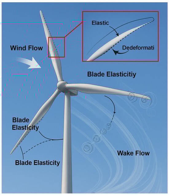
Figure 1.
Coupled aerodynamic–structural behavior of wind turbine blades.
The S809 airfoil profile was chosen for modeling the turbine blades. The detailed blade design methodology was outlined in earlier published papers by Alkhabbaz et al. [22]. A summary of the remaining design parameters is provided in Table 1. An iterative approach is applied to solve the BEM, utilizing Equations (1)–(4) to determine the optimal blade profile:

Table 1.
The design parameters of proposed 2 kW wind turbine.
The twist angle () indicates the variation between the actual flow angle and the intended design angle of attack at each blade section. Figure 2 depicts the obtained blade profile in terms of chord length and twist angle distributions.
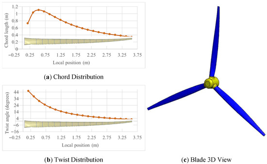
Figure 2.
Geometric characteristics of the wind turbine blade.
3. Modeling of Wind Turbine
3.1. Flow Domain and Boundary Conditions
The radius of the turbine rotor (R) was a doped as a characteristic length to create the flow domain. It has two subdomains: one stationary region, which models the overall flow field, and a rotating one, containing the turbine blades. The sliding mesh technique is used to model the rotation of the blades. The extension of the computational domain is made just large enough to reduce the effects of the wake and the echo of the boundary: it extends 3R upstream of the rotor plane, 9R downstream, and 6R laterally, as shown in Figure 3.
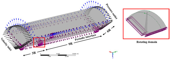
Figure 3.
Flow field with rotating domain and boundary conditions.
The upstream boundary has a uniform velocity inlet, and the downstream end of the domain has a static pressure outlet. The non-slip wall condition was set for the turbine blade. In order to take advantage of the symmetry of a three-blade rotor, only a sector of the domain is modeled, and periodic boundary conditions are applied along the circumferential side [23]. Such methodology greatly minimizes the expense of computation and accuracy in the assessment of aerodynamic loads and the development of wakes. The rotating domain, indicated in the inset, encloses the rotor, and it is attached to the fixed flow field through the sliding mesh interface. This setup ensures accurate resolution of the unsteady flow structures induced by blade rotation and wake evolution.
3.2. Numerical Scheme and Mesh Topology
The aerodynamic performance of the wind turbine blade was numerically investigated using the ANSYS-CFX (2023-R1) commercial solver. The governing incompressible Navier–Stokes equations were resolved through the finite volume method with pressure–velocity coupling to ensure conservation of mass. A semi-implicit algorithm in combination with a second-order upwind discretization scheme was employed to achieve numerical stability and accuracy in capturing flow gradients. Although the Navier–Stokes equations theoretically provide a complete description of turbulent flows, resolving all flow scales in a complex three-dimensional domain at high Reynolds numbers remains computationally prohibitive with current resources. To address turbulence modeling, the shear stress transport (SST) k–ω model with an inlet turbulence intensity of 0.05 was adopted, as it provides reliable predictions of boundary-layer behavior, particularly in regions with strong gradients and flow separation [24,25,26,27]. This model is well-suited for capturing unsteady flow features and turbulence structures around the rotor blades and the surrounding domain, owing to its effective dissipation representation in the transport equations [28].
Mesh generation plays a crucial role in solving the governing equations of fluid flow within complex geometries. In the present work, the CFD simulations were carried out using fully structured hexahedral meshes created with the ANSYS-ICEM software (2023-R1). Locally refined mesh areas were also added to the turbine blades and the diffuser to enable proper handling of the flows and thus increase the level of reliability of the aerodynamic predictions. The focus was placed on the boundary layer, and the 12 prism layers were formed near the blade surfaces, and the normal growth ratio was applied, with the starting layer thickness of 0.02 mm and ending with the layer thickness of 1.2 mm. The entire computational grid will be broken down into two separate areas: a rotating area, which will consist of the blades and hub, and a stationary area, representing the rest of the flow field, as shown in Figure 4. These domains were interlocked with a sliding mesh interface that allowed representation of the rotor flow interaction to be accurate.
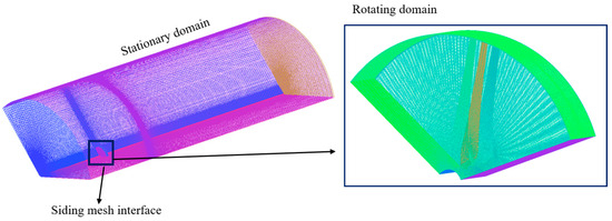
Figure 4.
Structured mesh topology of the computational domain.
A mesh independence test was performed to ensure that the selected mesh strikes a balance between computational cost and result accuracy. It also confirmed that the outcomes were not influenced by the specific mesh size used. Six different mesh resolutions were used, with each level increasing by 50% to ensure a reliable mesh convergence test. This test was conducted on the suggested wind turbine blade at the highest incoming wind speed of 12 m/s, a condition under which complex aerodynamic behavior and wake flow can be well represented. The test results showed that at the initial stage, with around 1 million mesh elements, the aerodynamic performance of the wind turbine blade, specifically the power output, was relatively low due to the coarse mesh resolution. As the mesh became progressively finer, the power output increased, eventually reaching a point where further refinement no longer had a noticeable impact on result accuracy, as illustrated in Figure 5. Based on these findings, the final mesh consisting of approximately 2.46 million hexahedral cells was chosen for the rest of the simulations, offering a high enough resolution to accurately capture the complex flow structures.
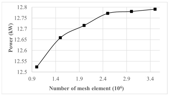
Figure 5.
Convergence of power output with mesh element count.
3.3. Code Validation
Numerical validation was carried out to assess the fidelity of a computational representation and to quantify the deviation between the predicted outcomes of the model and the actual physical phenomena [29,30]. Figure 6 presents a comparison between the present CFD-based numerical simulations of the NREL Phase VI wind turbine and the experimental results reported by NREL [31] across a range of wind speeds. Figure 6a illustrates the power output trend, while Figure 6b depicts the corresponding thrust force trend. In both cases, the CFD predictions show very good agreement with the experimental measurements, confirming the reliability of the adopted numerical approach for aerodynamic performance evaluation. The power curve demonstrates a nearly linear increase, with wind speeds up to around 8–9 m/s, after which the growth rate moderates as aerodynamic and structural losses become more significant. A similar pattern is evident in the thrust curve, where thrust force rises steeply at lower wind speeds and gradually levels off at higher wind speeds, consistent with the onset of flow separation and stall effects.
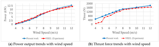
Figure 6.
Verification of wind turbine aerodynamic behavior.
The trends of power and thrust are also correlated in an interesting way that can be observed. The power and thrust growth go hand in hand with the increase in wind speed, meaning that a proportionate growth in energy extraction is necessarily accompanied by an increase in the aerodynamic load on the rotor. The CFD models are inclined to have a minor overprediction of thrust at higher wind speeds as compared to the experiments, but the power prediction is close. This small difference could be explained by the simplification of the modeling of turbulence closure, the roughness of the blades’ surface, or the three-dimensional stall effects that are difficult to represent by numerical models due to their nature. However, the general consistency of the simulation with the experimental data confirms the current methodology of CFD and highlights its ability to predict the energy performance of the NREL Phase VI wind turbine as well as its aerodynamic loading features in a reliable and suitable way.
4. Artificial Neural Networks
Artificial neural networks (ANNs) have shown remarkable effectiveness in a wide range of engineering problems thanks to their adaptability and self-learning capability [18]. Among the commonly used structures is the multilayer perceptron (MLP), which belongs to the family of feedforward neural networks. A standard three-layer MLP consists of an input layer with m nodes, a hidden layer with z neurons, and an output layer with n nodes. Each hidden neuron connects to all inputs, and every output neuron receives input from all hidden units. As illustrated in Figure 7, and represent input and output variables, and is the hidden layer output, while the weights between the layers are denoted by (input-to-hidden) and (hidden-to-output).
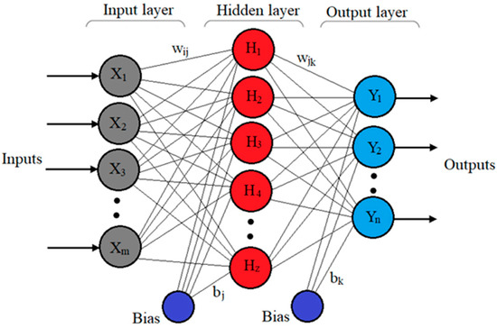
Figure 7.
Multilayer perceptron architecture comprising a single hidden layer with z neurons.
The input to the j-th neuron in the hidden layer can be calculated based on the input from the i-th neuron in the input layer, as follows:
where and refer to the neurons in the input and hidden layers, respectively. The bias term for the hidden layer is represented by . To process the input signals, the hidden layer uses the logistic sigmoid function as its activation function. The mathematical form of the logistic sigmoid function is given by the following:
After applying the activation function, the output of the j-th neuron in the hidden layer is computed as follows:
The signals transmitted from the hidden layer to the output layer are processed through the following mathematical expression:
where k is an index of an output neuron. Also, denotes the bias for the output layer. The activation function for the output layer of the developed feedforward neural network model is a linear function (purelin). Mathematically, it is represented as follows:
Following the activation function, the output of the k-th neuron in the output layer is determined using the following expression:
When values corresponding to the target and the projected output vector do not match, the output ‘errors’ are processed ‘backward’ in the output layer. This technique, which allows for the reduction in overall inaccuracy, makes it possible to adjust weights in every layer. The following describes the output and hidden layer corresponding error terms:
The update rules for adjusting the biases and weights are given as follows:
where Tk represents the actual output value, while α denotes the learning rate.
Many different methods of ANNs have been documented in the literature. Based on extensive surveys, the most used methods are the scaled conjugate gradient (SCG) method, Levenberg–Marquardt backpropagation (LM), and resilient backpropagation (RP) methods [32]. It is widely accepted that the LM method is one of the most effective methods in training neural networks since it numerically solves the minimization of nonlinear functions. It alleviates the problems of the Gauss–Newton algorithm and the gradient descent approach by synergizing the two, thus offering fast and stable convergence. It is recommended for small-to-medium ANN models [33]. The initial step of the LM process uses steepest descent to arrive near the solution in the high-curvature regions and then evens out the parameters until there is local curvature and an accurate quadratic fit is maintained. The next step involves utilizing the Gauss–Newton method to refine the answer and extend the solution further. The next step involves calculating the total squared error for each training instance and the respective output of the neural network from the formula below:
where denotes the training error margin, which is associated with the outputs corresponding to the z input pattern, and is mathematically expressed as follows:
where and indicate the actual and target output vectors, respectively. Typically, the gradient g is widely described as the first derivative of the total error function:
Once the gradient g is determined, the update rule for the steepest descent algorithm can be stated as follows:
The update formulas for both the Gauss–Newton algorithm and Newton’s method are given as follows:
The training, Hessian, and Jacobian matrices are denoted separately as , , and The approximate Hessian matrix JTJ is invertible. The Levenberg–Marquardt (LM) method can be interpreted as a development of this approach in this direction and is defined as follows:
Here, μ is a positive scalar known as the combination coefficient, and I is the identity matrix. Based on this, the upcoming update rule for the LM algorithm is as follows:
Extensive information about the Levenberg–Marquardt algorithm can be found in the studies that were carried out by Johnson et al. [34].
Based on the aforementioned, Figure 8 illustrates the ANN configuration developed to predict the wind turbine power, based on selected input variables. The network architecture consists of three layers: an input layer with two neurons (wind speed and pitch angle), a hidden layer of six neurons, and a single-neuron output layer responsible for estimating output power. Using MATLAB 2021b [35,36], several ANN architectures were generated and tested to identify the optimal model, with the number of hidden layer neurons during training, before selecting the six-neuron configuration for best accuracy. The Levenberg–Marquardt (LM) learning algorithm was employed to train all the models. The various combinations of logsig, tansig, and purelin were considered, and the most accurate combination was selected for the final model. In this case, logsig was used as the logistic sigmoid function in the hidden layer, and purelin, as the linear transfer function, was used in the output layer to yield the most optimal results.
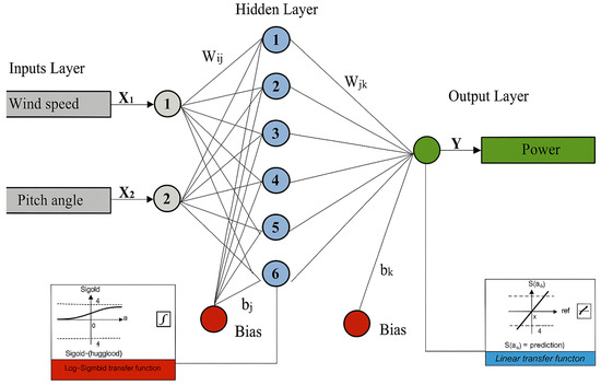
Figure 8.
The structure of the adapted ANN model.
5. Error Analysis Parameters
This study developed an ANN model based on a feedforward multilayer architecture. A total of 70% of the CFD simulation data for wind turbines was used for model training, and the remaining 30% for testing and validation. This network consists of two input neurons (for pitch angle and wind speed, respectively), a hidden layer of six neurons, and an output neuron (for output power). Sensitivity analysis was used to increase the number of hidden layer neurons from three to fifteen, selecting the configuration with the minimum mean squared error (MSE) and the maximum correlation coefficient (R) to determine the optimal number of hidden layer neurons. Model performance was evaluated based on mean absolute error (MAE), root mean square error (RMSE), mean squared error (MSE), and correlation coefficient (R). The formulas for these metrics are listed below [37]:
where denotes the true (observed) value, while yi denotes the predicted value. The variable n represents the total number of data samples used in the training or testing phases.
6. Results and Discussion
A high-fidelity computational fluid dynamics simulation explores how adjusting the blade pitch angle modifies the integrated aerodynamic performance and aeroelastic reaction of a 2 kW horizontal-axis wind turbine through a wide wind-speed range. Simulations cover the profile from a 4.5 m/s cut-in speed to a 12.5 m/s cut-out speed, configuring pitch angles from to . A side-by-side simulation of multiple pitch settings allows an assessment of how controlled blade twist alters aerodynamic behavior. Blade-wise and overall blade deformation, along with blade-tip deflection, show pressure distribution and conform to contour depiction, supporting parameters of interest, which include aerodynamic torque, power coefficient, and thrust coefficient. This comprehensive turbine performance characterization augments a clear quantitative turbine performance assessment with a distinct quantitative turbine performance evaluation under various loading and pitch conditions.
6.1. Influence of Blade Pitch Angle on Aerodynamic Performance of the Rotor
The aerodynamic behavior of a wind turbine blade at 2 kW was simulated at a range of approaching wind speeds, between the cut-in speed of the turbine, 4.5 m/s, and the cut-out speed, 12.5 m/s. These velocities were maintained between 4 and 11 tip-speed ratios and the constant rotational speed of the turbine was maintained at 200 rpm. The correlation between wind speed and the aerodynamic torque at the constant pitch angle of , and is shown in Figure 9. The torque is augmented by the wind speed up to a peak based on the accumulated wind kinetic energy. The peak torque is reached at a pitch of with lower speeds of less than 10 m/s. The angle of attack in this case is the closest to the theoretical optimum one, with the highest lift-to-drag ratio, which improves aerodynamic efficiency. On the other hand, the datum at pitch represents an optimum angle of attack, which provides a relatively low value of lift-to-drag ratio and, therefore, represents the minimum torque in the test range.
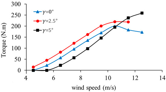
Figure 9.
Aerodynamic torque response at different pitch angles.
Beyond a wind speed of 10 m/s, alteration of the pitch angle begins to produce an impact significant to the aerodynamic behavior, with a peak torque occurring at of pitch. This action implies that when at high speeds, even a slight movement in the direction of pitch actually postpones the commencement of stall on the blade, thereby sustaining a greater level of torque and increasing efficiency. This observation enables feasible pitch optimization that is associated with wind climate: the lowest angles are observed to maximize the energy in light-to-moderate events, but, on the other hand, high angles act to counter-stall, shield the apparatus, and encourage continuous power output on stronger gusts.
Figure 10 shows a correlation between the power coefficient and the tip-speed ratio of a wind turbine when the rotational speed is held constant (200 rpm), and the pitch angle varies . At low (under 4–5), grows, slowing up to all pitch angles. This phenomenon is due to the fact that when the speed of a blade at the tip of the blade is relatively low, relative to the approaching wind, and the blades cannot provide adequate lift, leading to low aerodynamic efficiency. The aerodynamic conditions surrounding the blades increase with the increase in the , which increases the lift generation and makes the utilization of more energy possible. The highest is found at moderate levels of at around 6–7. At this distance, is approximately 0.42 in the case of , 0.36 in the case of and 0.28 in the case of . The excellent performance of shows that blades that are oriented in close proximity to the flow can have the highest aerodynamic efficiency. On the contrary, a higher pitch angle decreases the effective angle of attack, thus facilitating an early separation of flow and decreasing the maximum attained. In all cases, declines beyond values of 8. When the ratios are at these high levels, the blade tips become too fast in reference to the wind, thereby augmenting the drag and reducing aerodynamic efficiency. This decline is strongest at which is where decreases rapidly, and the number approaches zero at = 10. Smaller pitch angles result in behavior that can be associated with aerodynamic stall and blade-flow misalignment.

Figure 10.
Power coefficient response at different pitch angles.
The present results show a maximum of approximately 0.42 at , which is slightly lower than that of commercial designs. This implies that the turbine’s efficiency can be improved further with better blade design or sophisticated pitch-control systems, even though the turbine’s configuration is efficient enough. In addition, the naturally diminishing value at higher TSR levels can be useful in preventing excessive power capture during high-wind situations. Thus, the ability to change the pitch angle is a vital control feature: lower pitch angles enhance efficiency with average winds, while higher pitch angles restrict structural loads during strong winds.
With a rotor speed of 200 rpm, the thrust coefficient changes with TSR, as presented in Figure 11. is a critical aerodynamic indicator of the thrust and represents the axial force on the rotor as a part of the incoming rotor wind. This parameter is important, as it impacts the performance of the turbine and also directly impacts the structural loading of the blades, the tower, and the drivetrain. At low TSR values, increases in TSR. This demonstrates that in instances of low blade-tip speeds, the thrust produced is low, owing to the rotor having weak-to-moderate interaction with the incoming flow. With an increase in TSR, the rotor blade aerodynamics are enhanced, resulting in a stronger lift force in addition to an increase in rotor axial loading. generally, has a peak value in moderate TSR regions. This peak value defines the rotor’s energy extraction efficiency, which is optimal, but there is simultaneous peak axial loading. This maximum value is a function of the pitch angle of the blade: lower pitches have a greater thrust because the blades align better with the wind. Increasing pitch angles cause the effective angle of attack to decrease, and therefore, reducing the aerodynamic loading experienced, resulting in a lower peak .
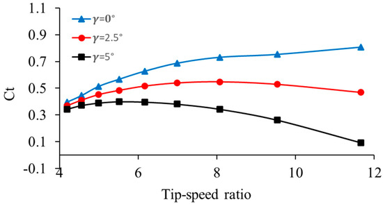
Figure 11.
Thrust coefficient response at different pitch angles.
At higher values of TSR, sharply recedes. When the tip of the blade rotates at a much faster rate than the wind is coming, a drag-and-flow separation will occur, resulting in a reduction in the axial force that is sent to the rotor. This reduction is greater with larger pitch angles due to greater blade misalignment, which limits the aerodynamic loading. The turbine’s aerodynamic and structural behavior is revealed while observing the and TSR relationship. The rotor and tower face significant axial loading when high thrust coefficients are applied, which need to be controlled to prevent fatigue and structural damage. The trends in the results are in line with what is expected: increases with TSR to a peak and subsequently declines. This is helpful in practice as the reduction in with higher TSR values helps prevent turbine damage due to strong winds, minimizing the chances of mechanical overload. Additionally, the application of pitch control enables the operators to adjust the thrust loads to desired levels: small pitch angles increase thrust and energy capture during moderate wind conditions, and bigger pitch angles decreases loads during storms or high-wind periods for improved safety. It is equally important from the engineering point of view to know the –TSR relation for optimally balancing the structure’s performance and reliability. A well-functioning turbine has to optimally keep TSR at its ideal range to ensure a high energy yield, and the natural decrease in at high TSR provides some level of protective mechanism by reducing stress on the structure. For this reason, the thrust coefficient is more than an aerodynamic loading parameter, and unsurprisingly, an important variable for turbine reliability.
6.2. Influence of Blade Pitch Angle on Structural Elasticity of the Rotor
The second focus of the present simulation is the assessment of the structural response of the blade under different loading conditions and pitch angles, with the aim of comparing its mechanical performance. A one-way aeroelastic analysis was carried out for the blade configuration across a broad range of wind speeds. In this approach, the steady aerodynamic loads, including gravitational effects, were first obtained from CFD simulations and subsequently applied to the structural model in ANSYS 2023R1. Using these inputs, some of the critical structural parameters, like maximum deflection of the blade tip, the equivalent stress distribution, and general longitudinal deformation, were analyzed in relation to wind speed in order to describe the structural behavior of the blade.
Figure 12 shows the variation in blade-tip deflection versus the incoming wind speed at a constant rotational speed of 200 rpm, at three different pitch angles . These findings indicate that there is an evident dependency of structural deformation on wind speed and pitch setting. When the deflection is greatest, and it is almost 26 mm at 12 m/s. The reason is that the blade at the zero pitch achieves maximum aerodynamic force, resulting in increased bending moments and increased structural deformation. The higher the angle of pitch, the lower the tip deflection at the same wind speed is, as the pitch angle is and . The cause of this reduction is that the higher the angle of pitch, the smaller the effective angle of attack and, therefore, the smaller the lift forces acting on the blade, and, accordingly, structural bending is minimized. Aeroelasticity-wise, the nonlinear trend of the curves implies that the deflection of the tip is more pronounced within the lower ranges of wind speeds (between 4 and 10 m/s), and then the curve slows down. This is the combined action of aerodynamic loading as well as structural stiffness. With the blade deflection, there is a slight change in aerodynamic characteristics, which is a kind of passive load relief as a result of geometric nonlinearity. Additionally, the trade-off between aerodynamic efficiency and structural safety is also seen in the comparison of the three pitch angles: the smaller the pitch angle, the more aerodynamic power it can extract and the greater the de-flections it induces, and vice versa.
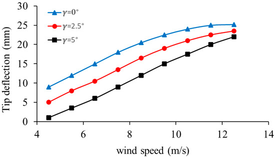
Figure 12.
Effect of wind speed and pitch angle on blade-tip deflection.
According to the above, Figure 13 offers a complementary view by revealing the maximum pressure load distribution on the blade surface at the same angle of pitch and three wind speeds. The findings depict that maximum pressure load increases with an increase in wind speed, irrespective of the pitch angle, as observed in the deflection of the tip. In the lower range of wind speed (V = 4.5 m/s), the pressure loads are small (1200 Pa), whereas in higher wind speeds (V = 12.5 m/s), loads are higher than 1600 Pa and directly proportional to the higher tip bending observed above. The effect of the pitch angle can also be observed: when , the pressure loading tends to make the maximum, and this is why the tip deflection in Figure 12 was the most significant in this situation. Peak pressure loads minimally decrease when pitch angle rises to and , and this is also in agreement with the decreased structural deflection. This means that the elastic response of the blade is directly proportional to the pressure load distribution, which proves that tip deflection is a structural impact of aerodynamic loading.
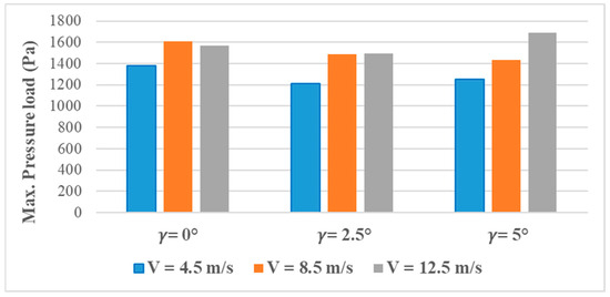
Figure 13.
Max pressure load distribution on the blade surface.
The change in Von Mises stress in the blade with the wind speed and pitch angle is indicated in Figure 14. The stress levels are fairly constant at and at various wind speeds, despite the fact that the pressure loads are increasing, as demonstrated above. It means that even though aerodynamic pressure and tip deflection increase with the speed of wind, the structure of the blade can redistribute the induced loads effectively at these lower pitch angles and prevent a significant increase in stress. But at , one can distinctly see in the trend that the Von Mises stress grows more steeply, almost approaching 8 MPa at V = 12.5 m/s. This behavior can be explained in light of the pressure load distribution (Figure 13). While higher pitch angles reduced the aerodynamic pressure loads and tip deflections, they also changed the load path and structural stiffness interaction within the blade. The reduction in aerodynamic forces limits excessive bending, but it shifts the stress concentration toward material-level responses, leading to increased internal stress under high wind speeds.
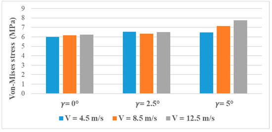
Figure 14.
Von Mises stress distribution on the blade surface.
6.3. Performance Analysis of ANN in Predicting Aerodynamic Performance
At , Figure 15 compares the actual power output of the wind turbine blade obtained from CFD analysis with the outputs of an ANN model. For the wind-speed range of 4–12 m/s, both curves demonstrate an increasing trend, indicating that the ANN model was able to capture the power output to wind speed dependence from the CFD data. For the ranges of 4–6 m/s, the ANN underestimation of CFD data was predominant. In the range of 8–10 m/s, the agreement reaches a very close value. The region of wind speed 11–12 m/s showcases an opposing phenomenon where the ANN outputs were higher than the CFD data. The general trend, however, was the same, highlighting its value as a surrogate model for CFD.
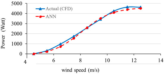
Figure 15.
ANN predictions against CFD data at blade pitch angle (0°).
Figure 16 compares the CFD-based actual power output with the predictions from the ANN model for a wind turbine blade at a pitch angle of 2.5°. For wind speeds ranging from 4 to 12 m/s, the power output, for both curves, continues to power, suggesting favorable turbine aerodynamics. ANN underestimates the CFD data, but only for the lower speeds of 4–6 m/s. For the midrange of 8–10 m/s, the ANN predictions are nearly equal to the CFD, suggesting that the model is capturing the nonlinear trend. For the higher speeds of 11–12 m/s, the ANN is still acceptable, but the CFD data is being underestimated. Overall, the ANN is still a dependable approximation for the CFD output, confirming its value as a surrogate model.
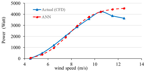
Figure 16.
ANN predictions against CFD data at blade pitch angle (2.5°).
An analysis of CFD’s actual power output and the predicted power output based on the ANN model on a wind turbine blade at a pitch of 5° is illustrated in Figure 17. As the wind speed rises from 4 to 12 m/s, both CFD and ANN curves are expected to become higher at a power output. During the periods of low wind speed (4–6 m/s), the ANN estimates CFD results tracking fairly closely with minimal divergence. During midrange wind speed (8–10 m/s), the ANN maintained a strong correlation with CFD and followed the outline of the CFD curve. During the higher wind-speed range (11–12 m/s), the CFD results are predicted by the ANN model, and the divergence rises. Overall, this pattern indicates that the ANN approach successfully estimates the power output of the turbine and wind speed using CFD as a source of data.
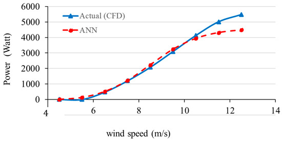
Figure 17.
ANN predictions against CFD data at blade pitch angle (5°).
Given the comparison between CFD and ANN results at the three pitch angles of it is evident that at a pitch angle of , the ANN seems to outperform its other predictions. Bundled at this pitch angle is the achievement of the least deviation; thus, the average error is characterized as being 5 to 7, which is lower than both the 0 and the 5 results. The predictions at were almost exact, which means that the dataset at that angle might have been more balanced. The model, however, at pitch angle appears to over-predict the power at higher wind speeds, and at a pitch angle, the model under-predicts the CFD outputs. Hence, it is more evident that the predictions have higher deviation. Thus, it can be concluded that the ANN model works the best at the 0.5 pitch angle, as the data shows the flow characteristics are stable and the predictions more reliably fit the training data.
To evaluate the prediction accuracy, the statistical error margin of the considered method is calculated. The ANN achieved superior performance on the testing data, with MAE and RMSE of 0.0272 and 0.0325, respectively, and an excellent match with a coefficient of R = 0.9957. These results prove the ANN’s robustness and reliability as an alternative model for computationally expensive CFD simulations in predicting the output power of wind turbines.
Figure 18 shows how the model outputs compare with the actual power outputs from the ANN model. The proximity of the data points to the 1:1 reference diagonal is indicative of strong conformity between the model’s predictions and the actual experimental results. The regression line also closely follows the reference line with R2 = 0.9957, certifying excellent predictive capability. Small deviations between the two lines suggest minimal prediction error across the sample range. Overall, the ANN model provides reliable estimates of the power output of the wind turbine and confirms that the predictions are validated with high confidence.
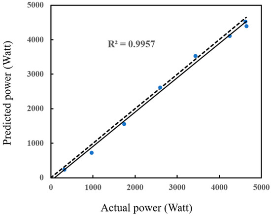
Figure 18.
The coefficient of determination (R2) regression between the predicted power value and the actual power value.
6.4. Structural Response of Wind Turbine Blades to Aeroelastic Loading
Figure 19 shows a comparison between the predicted blade deformation from the ANN model and the results from high-fidelity CFD simulations at a blade pitch angle of . As wind speed increases, both the ANN and CFD data reveal a clear upward trend in blade deflection, reflecting the nonlinear increase in deformation due to rising aerodynamic loads. The comparison shows that the ANN model is tightly correlated to the given two approaches, and the deformation patterns observed in the ANN model are closely similar to the deformation patterns observed in the CFD results. The variations among the ANN forecasts and CFD results are also insignificant throughout the range of the tested wind speeds, particularly at the speed of 6–10 m/s, where the disparity is virtually non-existent. Although the ANN model predicts a little high at high wind speeds (more than 12 m/s), this is quite small and could be explained by the weaknesses of data-driven models in extrapolation outside of their training range.
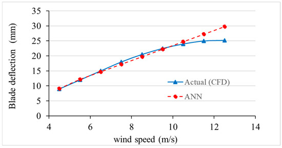
Figure 19.
Blade deformation predictions against CFD data at blade pitch angle (0°).
Figure 20 indicates that the predicted values of deformation using the ANN model are close to CFD values, with slight variations across the entire range of wind speeds (4–13 m/s) at a . This excellent observation establishes the fact that the ANN is an accurate model of the aero-structural coupling behavior of the system. The increased accuracy at compared with, say, the case in Figure 18 may be attributed to a more steady aerodynamic response and the less nonlinear effects of compared with the case. The ANN model is effective in the generalization of the deformation trend, and the results are in close correlation with the CFD, and the deviation in prediction is less than 3 percent, which is acceptable in engineering application.
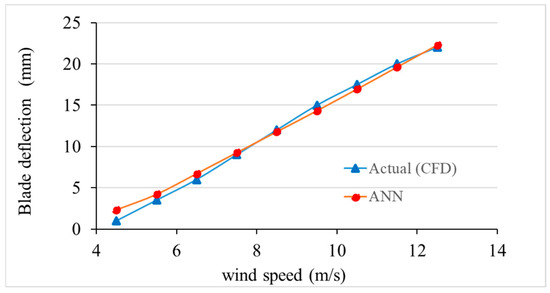
Figure 20.
Blade deformation predictions against CFD data at blade pitch angle (5°).
Figure 21 demonstrates the distribution of the pressure load along the blade span at three pitch angles at varying wind speeds. In general, as wind speed rises, the aerodynamic pressure on the blade surface also increases, regardless of the pitch angle. This occurs because higher wind velocity accelerates the airflow over the suction side, reducing static pressure, while the pressure side simultaneously experiences an increase in static pressure. The growing difference between these two regions leads to a greater overall pressure load. Additionally, increasing the pitch angle raises the effective angle of attack. As a result, the suction side encounters lower pressure and the pressure side receives higher pressure, which further amplifies the pressure differential across the blade surface, as shown in Figure 20.
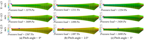
Figure 21.
Pressure distribution on blade surface at various wind speeds and pitch angles.
Figure 22 depicts the Von Mises stress contours of the proposed wind turbine blade for three pitch angles under different wind speeds. Von Mises stress represents the combined effect of normal (bending) and shear (torsion, shear flow) stresses. In blades, it peaks where bending moment and stiffness transitions are largest, typically near the root region. Increasing wind speed raises the external aerodynamic work. Therefore, it can be observed that the higher surface pressures were at higher wind velocities, and the deflection curve showed larger blade bending (Figure 13). Those larger aerodynamic loads and global deformations translate directly into higher material stress in Figure 14. At and , the increase with wind speed is modest because the blade’s greater flexibility at low pitch provides passive load alleviation (bend-induced reduction in effective angle of attack), slightly tempering the growth of stress even as loads rise.
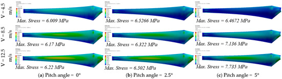
Figure 22.
Distribution of Von Mises stress on blade surface at various wind speeds and pitch angles.
Figure 23 and Figure 24 demonstrate how wind speed and blade pitch angle influence the aeroelastic behavior of the small-scale wind turbine blade, with particular focus on overall deformation and tip deflection. At lower wind speeds, such as 4.5 m/s, both parameters remain minimal, whereas higher wind speeds (8.5 m/s and 12.5 m/s) lead to a marked increase as a result of intensified aerodynamic forces. The influence of the pitch angle is also evident; the highest deformation and tip deflection are observed when the blades are placed at this is the most intense aerodynamic loading. By slightly changing the pitch angle to and then to the responses of the structure are significantly minimized, and this demonstrates the importance of pitch regulation in the mitigation of mechanical stresses. This practice proves the fact that the control of the pitch is not only necessary to maximize the energy capture, but also to reduce the structural strain with the aim of enhancing the operational reliability and the life of the turbine in various wind conditions.
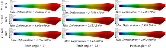
Figure 23.
Distribution of blade deformation at various wind speeds and pitch angles.
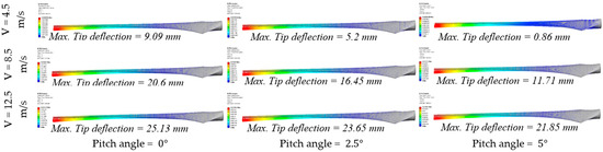
Figure 24.
Distribution of tip deflection of the blade at various wind speeds and pitch angles.
7. Conclusions
This study presented an integrated framework combining computational fluid dynamics (CFD) simulations with artificial neural networks (ANNs) to predict the aerodynamic performance and aeroelastic response of a small-scale wind turbine blade. The novelty of this work lies in leveraging ANN as a surrogate model for CFD, thereby reducing computational cost and time while maintaining high prediction accuracy. The CFD simulations provided detailed insights into aerodynamic loads, blade deformation, and stress distributions under varying wind speeds and pitch angles, forming a robust dataset for training the ANN. In turn, the ANN demonstrated excellent predictive capability, achieving deviations as low as 5–7% from CFD results at optimal pitch angles, thereby validating its effectiveness as a reliable surrogate. The results further revealed that the maximum power coefficient reached 0.42 at pitch, while blade-tip deflection decreased by nearly 60% when the pitch was increased to , underscoring the trade-off between aerodynamic efficiency and structural stability. Additionally, the ANN reduced the computational demand by approximately 50%, proving its viability for rapid performance evaluation. These findings highlight the strength of this hybrid CFD-ANN approach as an innovative, efficient, and accurate method for advancing wind turbine design and optimization, contributing to safer, more cost-effective, and sustainable renewable energy solutions.
Author Contributions
Methodology and writing original draft, H.H.; Software and writing original draft, A.A.; Validation, A.K.; Investigation, L.M.J.; Investigation, I.K.A.; Investigation, A.H.Y.; writing original draft, H.-S.Y.; Supervision, Y.-H.L.; Funding acquisition, Y.-H.L. All authors have read and agreed to the published version of the manuscript.
Funding
This research was supported by Korea Institute of Energy Technology Evaluation and Planning (KETEP) grant funded by the Korean government (MOTIE) (20213000000030), Development of disconnectable mooring system for A MW class floating offshore wind turbine.
Institutional Review Board Statement
Not applicable.
Informed Consent Statement
Not applicable.
Data Availability Statement
The original contributions presented in this study are included in the article. Further inquiries can be directed to the corresponding author.
Conflicts of Interest
The authors declare no conflict of interest.
Nomenclature
| List of symbols | ||
| Symbol | Unit | Definition |
| C | Chord length | |
| - | Drag coefficient | |
| - | Power coefficient | |
| - | Thrust coefficient | |
| Rotor diameter | ||
| - | Number of blades | |
| - | Number of elements | |
| Power | ||
| Rotor radius | ||
| Local radius | ||
| List of abbreviations | ||
| Symbol | Unit | Definition |
| Angle of attack | ||
| Twist angle | ||
| Blade pitch angle | ||
| - | Tip-speed ratio | |
| - | Local tip-speed ratio | |
| Angle of relative wind | ||
| Angular velocity | ||
References
- Leung, D.Y.C.; Yang, Y. Wind energy development and its environmental impact: A review. Renew. Sustain. Energy Rev. 2012, 16, 1031–1039. [Google Scholar] [CrossRef]
- Liu, M.; Tan, L.; Cao, S. Theoretical model of energy performance prediction and BEP determination for centrifugal pump as turbine. Energy 2019, 172, 712–732. [Google Scholar] [CrossRef]
- Global Wind Report. Global Wind Energy Council. 2022. Available online: https://klimaatweb.nl/wp-content/uploads/po-assets/747206.pdf (accessed on 26 September 2025).
- Ahlström, A. Influence of wind turbine flexibility on loads and power production. Wind Energy 2006, 9, 237–249. [Google Scholar] [CrossRef]
- Chou, J.-S.; Chiu, C.-K.; Huang, I.-K.; Chi, K.-N. Failure analysis of wind turbine blade under critical wind loads. Eng. Fail. Anal. 2013, 27, 99–118. [Google Scholar] [CrossRef]
- Kariman, H.; Hoseinzadeh, S.; Khiadani, M.; Nazarieh, M. 3D-CFD analysing of tidal Hunter turbine to enhance the power coefficient by changing the stroke angle of blades and incorporation of winglets. Ocean. Eng. 2023, 287, 115713. [Google Scholar] [CrossRef]
- Chen, X.; Li, C.F.; Xu, J.Z. Post-mortem study on structural failure of a wind farm impacted by super typhoon Usagi. In Proceedings of the EWEA Annual Conference and Exhibition 2015, Paris, France, 17–20 November 2015. [Google Scholar]
- Li, Z.; Chen, S.; Ma, H.; Feng, T. Design defect of wind turbine operating in typhoon activity zone. Eng. Fail. Anal. 2013, 27, 165–172. [Google Scholar] [CrossRef]
- Yu, D.O.; Kwon, O.J. Predicting wind turbine blade loads and aeroelastic response using a coupled CFD–CSD method. Renew. Energy 2014, 70, 184–196. [Google Scholar] [CrossRef]
- Bazilevs, Y.; Hsu, M.-C.; Kiendl, J.; Wüchner, R.; Bletzinger, K.-U. 3D simulation of wind turbine rotors at full scale. Part II: Fluid–structure interaction modeling with composite blades. Int. J. Numer. Methods Fluids 2011, 65, 236–253. [Google Scholar] [CrossRef]
- Dai, J.C.; Hu, Y.P.; Liu, D.S.; Long, X. Aerodynamic loads calculation and analysis for large scale wind turbine based on combining BEM modified theory with dynamic stall model. Renew. Energy 2011, 36, 1095–1104. [Google Scholar] [CrossRef]
- Mo, W.; Li, D.; Wang, X.; Zhong, C. Aeroelastic coupling analysis of the flexible blade of a wind turbine. Energy 2015, 89, 1001–1009. [Google Scholar] [CrossRef]
- Siavash, N.K.; Ghobadian, B.; Najafi, G.; Rohani, A.; Tavakoli, T.; Mahmoodi, E.; Mamat, R.; Mazlan, M. Prediction of power generation and rotor angular speed of a small wind turbine equipped to a controllable duct using artificial neural network and multiple linear regression. Environ. Res. 2021, 196, 110434. [Google Scholar] [CrossRef]
- Taghinezhad, J.; Sheidaei, S. Prediction of operating parameters and output power of ducted wind turbine using artificial neural networks. Energy Rep. 2022, 8, 3085–3095. [Google Scholar] [CrossRef]
- Nikolić, V.; Petković, D.; Shamshirband, S.; Ćojbašić, Ž. Adaptive neuro-fuzzy estimation of diffuser effects on wind turbine performance. Energy 2015, 89, 324–333. [Google Scholar] [CrossRef]
- Hjort, S.; Larsen, H. Rotor Design for Diffuser Augmented Wind Turbines. Energies 2015, 8, 10736–10774. [Google Scholar] [CrossRef]
- Ghorbani, M.A.; Shamshirband, S.; Zare Haghi, D.; Azani, A.; Bonakdari, H.; Ebtehaj, I. Application of firefly algorithm-based support vector machines for prediction of field capacity and permanent wilting point. Soil Tillage Res. 2017, 172, 32–38. [Google Scholar] [CrossRef]
- Tian, S.; Arshad, N.I.; Toghraie, D.; Eftekhari, S.A.; Hekmatifar, M. Using perceptron feed-forward Artificial Neural Network (ANN) for predicting the thermal conductivity of graphene oxide-Al2O3/water-ethylene glycol hybrid nanofluid. Case Stud. Therm. Eng. 2021, 26, 101055. [Google Scholar] [CrossRef]
- Ribeiro, A.F.P.; Awruch, A.M.; Gomes, H.M. An airfoil optimization technique for wind turbines. Appl. Math. Model. 2012, 36, 4898–4907. [Google Scholar] [CrossRef]
- Sun, H.; Qiu, C.; Lu, L.; Gao, X.; Chen, J.; Yang, H. Wind turbine power modelling and optimization using artificial neural network with wind field experimental data. Appl. Energy 2020, 280, 115880. [Google Scholar] [CrossRef]
- Manwell, J.F.; McGowan, J.G.; Rogers, A.L. Wind Energy Explained; John Wiley & Sons: Hoboken, NJ, USA, 2002. [Google Scholar] [CrossRef]
- Alkhabbaz, A.; Yang, H.-S.; Tongphong, W.; Lee, Y.-H. Impact of compact diffuser shroud on wind turbine aerodynamic performance: CFD and experimental investigations. Int. J. Mech. Sci. 2022, 216, 106978. [Google Scholar] [CrossRef]
- Kim, I.C.; Alkhabbaz, A.; Jeong, H.; Lee, Y.H. Optimization Methodology Of Small Scale Horizontal Axis Shrouded Tidal Current Turbine. In Proceedings of the 2019 IEEE Asia-Pacific Conference on Computer Science and Data Engineering (CSDE), Melbourne, VIC, Australia, 9–11 December 2019; pp. 1–3. [Google Scholar] [CrossRef]
- Bardina, J.; Huang, P.; Coakley, T. Turbulence Modeling Validation Testing, and Development; NACA technical memorandum; National Aeronautics and Space Administration (NASA): Moffett Field, CA, USA, 1997. [Google Scholar]
- Menter, F.R. Two-equation eddy-viscosity turbulence models for engineering applications. AIAA J. 1994, 32, 1598–1605. [Google Scholar] [CrossRef]
- Menter, F.R.; Kuntz, M.; Langtry, R. Ten Years of Industrial Experience with the SST Turbulence Model. Turbul. Heat Mass Transf. 2003, 4, 625–632. [Google Scholar]
- Hoffmann, K.A.; Chiang, S.T. Computational Fluid Dynamics Volume I. Engineering Education System; Engineering Education System (EES): Wichita, KS, USA, 2000. [Google Scholar]
- Alkhabbaz, A.; Hamza, H.; Daabo, A.M.; Yang, H.-S.; Yoon, M.; Koprulu, A.; Lee, Y.-H. The aero-hydrodynamic interference impact on the NREL 5-MW floating wind turbine experiencing surge motion. Ocean. Eng. 2024, 295, 116970. [Google Scholar] [CrossRef]
- Yang, H.-S.; Alkhabbaz, A.; Lee, Y.-H. Integrated CFD and hydrodynamic correction approach for load response analysis of floating offshore wind turbine. Ocean. Eng. 2025, 328, 121007. [Google Scholar] [CrossRef]
- Alkhabbaz, A.; Hamzah, H.; Hamdoon, O.M.; Yang, H.-S.; Easa, H.; Lee, Y.-H. A unique design of a hybrid wave energy converter. Renew. Energy 2025, 245, 122814. [Google Scholar] [CrossRef]
- Hand, M.M.; Simms, D.A.; Fingersh, L.J.; Jager, D.W.; Cotrell, J.R.; Schreck, S.; Larwood, S.M. Unsteady Aerodynamics Experiment Phase VI: Wind Tunnel Test Configurations and Available Data Comparisons; NREL/TP-500-29955; National Renewable Energy Laboratory (NREL): Golden, CO, USA, 2001. [Google Scholar]
- Geetha, A.; Santhakumar, J.; Sundaram, K.M.; Usha, S.; Thentral, T.M.T.; Boopathi, C.S.; Ramya, R.; Sathyamurthy, R. Prediction of hourly solar radiation in Tamil Nadu using ANN model with different learning algorithms. Energy Rep. 2022, 8, 664–671. [Google Scholar] [CrossRef]
- Hakim, G.P.N.; Hadi Habaebi, M.; Elsheikh, E.A.A.; Suliman, F.M.; Islam Md, R.; Yusoff, S.H.B.; Adesta, E.Y.T.; Anzum, R. Levenberg Marquardt artificial neural network model for self-organising networks implementation in wireless sensor network. IET Wirel. Sens. Syst. 2024, 14, 195–208. [Google Scholar] [CrossRef]
- Johnson, W.C.; Weinstein, A.; Charles, W. Electrical Engineering Handbook; CRC Press LLC.: Boca Raton, FL, USA, 2000; Volume 7, Available online: https://docs.preterhuman.net/The_Electrical_Engineering_Handbook (accessed on 26 September 2025).
- Canpolat, C.; Hamzah, H.; Sahin, B. Flow Control Around a Cylinder With a Perforated Cylinder. J. Fluids Eng. 2023, 145, 071302. [Google Scholar] [CrossRef]
- Yang, H.-S.; Alkhabbaz, A.; Lee, Y.-H. Toward Reliable FOWT Modeling: A New Calibration Approach for Extreme Environmental Loads. Energies 2025, 18, 5545. [Google Scholar] [CrossRef]
- Mateus, B.C.; Mendes, M.; Farinha, J.T.; Assis, R.; Cardoso, A.M. Comparing LSTM and GRU Models to Predict the Condition of a Pulp Paper Press. Energies 2021, 14, 6958. [Google Scholar] [CrossRef]


Disclaimer/Publisher’s Note: The statements, opinions and data contained in all publications are solely those of the individual author(s) and contributor(s) and not of MDPI and/or the editor(s). MDPI and/or the editor(s) disclaim responsibility for any injury to people or property resulting from any ideas, methods, instructions or products referred to in the content. |
© 2025 by the authors. Licensee MDPI, Basel, Switzerland. This article is an open access article distributed under the terms and conditions of the Creative Commons Attribution (CC BY) license (https://creativecommons.org/licenses/by/4.0/).