Abstract
Computing Shapley values for large cooperative games is an NP-hard problem. For practical applications, stochastic approximation via permutation sampling is widely used. In the context of machine learning applications of the Shapley value, the concept of antithetic sampling has become popular. The idea is to employ the reverse permutation of a sample in order to reduce variance and accelerate convergence of the algorithm. We study this approach for the Shapley and Banzhaf values, as well as for the Owen value which is a solution concept for games with precoalitions. We combine antithetic samples with established stratified sampling algorithms. Finally, we evaluate the performance of these algorithms on four different types of cooperative games.
Keywords:
cooperative game theory; permutation sampling; antithetic sampling; stratified sampling; Shapley value; Banzhaf value; Owen value MSC:
91A12; 91-08; 91-04
1. Introduction
Cooperative game theory [1,2] provides a framework for analyzing situations where groups of individuals or entities collaborate to achieve common goals or outcomes. Unlike non-cooperative game theory, which focuses on strategic interactions without binding agreements, cooperative game theory explores scenarios in which players can form coalitions and distribute the benefits of their cooperation.
Modern applications of cooperative game theory reach far beyond the fair allocation of benefits. For example, models and solution concepts from cooperative game theory are employed for understanding voting power in committees [3,4,5], as well as for analyzing genetic networks [6,7], terrorist networks [8,9,10], or complex shareholding networks [11,12]. However, for n players the number of coalitions grows exponentially and this makes efficient computations on cooperative games challenging. The latter is particularly true for the Shapley value [13], the most widely used solution concept from cooperative game theory. In the general case, calculating the Shapley value is NP-hard [14,15,16]. Very recently, there has been plenty of research in the field of interpretable machine learning using the Shapley value as a tool to determine the importance of features with respect to the outcome of neural networks [17,18,19,20]. In these applications, Shapley values are very frequently approximated via a technique called permutation sampling which was introduced in the seminal paper by Castro et al. (2009) [21]. Permutation sampling for Shapley value computation was improved in various ways in order to draw samples more efficiently [22,23,24]. In the machine learning community, antithetic sampling, i.e., employing a permutation together with its reverse, has gained traction due to its simplicity since it was recommended in an article by Mitchell et al. (2022) [23]. The recent survey by Chen et al. (2023) [18] presents antithetic sampling in a favorable light, and a recent book by Molnar (2023) [20] recommends antithetic sampling as well.
This paper studies antithetic permutation sampling for approximating Shapley values from a cooperative game theory perspective. Deliberately, we also include two other point-valued solution concepts in our investigations. The Banzhaf value [25,26] enjoys a wide range of applications, including contemporary studies on data valuation in machine learning [27]. The Owen value [28] generalizes the Shapley value for situations with precoalitions, i.e., the player set is partitioned into disjoint a priori unions of players. Algaba et al. (2023) [8] approximates Owen values to identify the most important people in the terrorist network responsible for the attack on the World Trade Center in September of 2001.
We incorporate antithetic sampling into existing algorithms for approximating the Shapley, Banzhaf, and Owen values. In particular, we also combine existing stratified sampling algorithms for the Shapley value [22] and for the Owen value [29] with the concept of antithetic sampling via the reverse permutation and develop new algorithms. We point out the unbiasedness and consistency of our estimators.
Our article is limited to point-valued solution concepts based on marginal contributions. For a study presenting Shapley value approximation in the broader context of computing solutions of cooperative games, we refer the reader to Liben-Nowell et al. (2012) [30]. Specifically, the goal of this research is to evaluate the potential of antithetic sampling in the context of sampling permutations or subsets with replacement. There are various other concepts for approximating Shapley values which this paper does not discuss, as it is too numerous to list them all. In particular, we do not perform any sampling without replacement [31,32] and we completely omit the multilinear extension method by Owen (1972) [33] and its recent variants [34], any approaches to combine sampling with exact solutions of subproblems [35,36], and any modern machine learning-related models [19,37].
This article is organized as follows: In Section 2, we introduce the basic concepts from cooperative game theory, provide a brief introduction to Monte Carlo methods and some variance reduction techniques, and give a very brief overview of existing permutation sampling algorithms. In Section 3, we discuss antithetic sampling for the Shapley and Banzhaf values, introduce a novel stratified antithetic sampling algorithm for Shapley value approximation, and point out how antithetic samples can be incorporated into the two-stage stratified sampling algorithm with optimum allocation introduced in [22]. In Section 4, we integrate antithetic sampling into the approximation algorithm for the Owen value introduced by Saavedra-Nieves, García-Jurado, and Fiestras-Janeiro (2018) in [38] and then develop a sophisticated stratified antithetic sampling method for the Owen value based on the ideas by Saavedra-Nieves from [29]. In Section 5, we analyze the performance of the discussed algorithms for four different types of cooperative games and assess the results critically. We end with our conclusions and recommendations in Section 6.
2. Preliminaries
In this section, we first introduce a few basic concepts from cooperative game theory, including the Shapley [13], Banzhaf [25,26], and Owen [28] values. Afterwards, we introduce some terminology on Monte Carlo methods, including variance reduction via antithetic sampling and stratified sampling.
2.1. Cooperative Game with Transferable Utility
The focus of our study is cooperative games with transferable utility (TU games) [1,2]. The term cooperative describes the fact that players can form coalitions and make binding agreements on how to distribute the proceeds of these coalitions between themselves. The term transferable utility means that the amount of utility earned by a coalition can be both expressed by a number and transferred between the players. The most common type of utility is money.
A TU game is a pair where is the set of players and is a real valued function, called the characteristic function, defined on the subsets of N. The subsets are also called coalitions. v maps a real number to each coalition S representing the amount of utility earned by this coalition. For the empty coalition there holds the normalization . Throughout this work, we will denote by a lower-case letter the cardinality of a set, e.g., .
Let be the set of TU games with player set N. A point-valued solution concept is a map that assigns a vector to each game , where the i-th element of this vector, , represents the worth or influence of player in the game according to the underlying solution concept. The most popular point-valued solution concept in cooperative game theory is the Shapley value [13]. Given the player set N and the characteristic function , the Shapley value of player i is defined as
Definition 1
([21,22]). Let denote the set of all possible permutations of the player set . Further, let be a permutation that assigns the player to each position k. Given a permutation , we define as the set of predecessors of player i in the order O, i.e., , if . In this setting, the marginal contribution of player ifor a given order is defined as .
Another important point-valued solution concept in cooperative game theory is the Banzhaf Value [25,26]. Given the player set N and the characteristic function , the Banzhaf value of player i is defined as
From (2) and (3), we understand that both Shapley and Banzhaf values are based on the concept of marginal contributions. Note that the Shapley value is an efficient solution concept as whereas in general the Banzhaf value is not, i.e., the sum of the Banzhaf values of all players does not necessarily equal the value of the grand coalition.
A TU game with precoalitions (also known as a priori unions) is a triple where is a TU game and is a partition of the player set N with p being the number of precoalitions. Each player has to be part of a precoalition, i.e., . Furthermore, all precoalitions are disjoint, i.e., for all and . We denote by the precoalition to which player i belongs. Throughout this work, we will use the terms precoalition, a priori union, and union as synonyms as long as there is no ambiguity. Likewise, we will use the terms partition and coalition structure synonymously.
We denote by a point-valued solution concept for games with precoalitions, where is the set of TU games with precoalitions with player set N. The most frequently used solution concept for cooperative games with precoalitions is the Owen Value [28]. It can be viewed as an extension of the Shapley value to games with precoalitions. Given the player set N, the characteristic function , and the partition P, the Owen value of player i is defined as
Just like for the Shapley value, it is also possible to write the Owen value in terms of permutations. We call a permutation compatible with a partition of the player set P if the elements of each class of P are never torn apart in the order O. Let denote the set of all permutations of N which are compatible with the coalition structure P. Then, the Owen value (4) of player i can be rewritten in the form
2.2. Monte Carlo Methods
Our introduction to Monte Carlo methods and permutation sampling follows Botev and Ridder (2017) [39] and Mitchell et al. (2022) [23]. Let , where is a discrete random variable following an equal distribution with being the sample space, and an arbitrary function that returns a real value for any value of its domain . The exact value of can be retrieved by evaluating
Using the crude Monte Carlo method [39], we can approximate as
with being drawn as i.i.d. replications of X and m being the number of samples. The resulting estimator is unbiased, i.e., , and its variance is given by
so that the variance shrinks with an increasing number of samples m, i.e., the estimator is consistent, as long as is finite.
Using Equation (2) and employing a uniform sample of permutations of size m delivers a simple Monte Carlo estimator for the Shapley value
This approach is called permutation sampling and was formally established by Castro et al. (2009) [21]. The estimator for the Shapley value of player i in (6) is unbiased and consistent. The Central Limit theorem guarantees convergence at a rate of . In terms of a practical implementation, a single sample of m permutations can be used to evaluate the Shapley values for all players i. We can walk through each permutation of length n and when incrementing i and evaluating we simply reuse from the previous computation [23].
Antithetic sampling is a variance reduction technique for Monte Carlo methods. Instead of taking i.i.d. samples, samples are taken as correlated pairs. The overview article [40] defines the antithetic estimate as
where is an i.i.d. sample and its corresponding antithetic sample. The variance of the estimator is given by
so that if and have a negative covariance, i.e., they are negatively correlated, the variance of the estimator is reduced compared to the crude Monte Carlo approach. Antithetic sampling for functions of permutations was first investigated in [41]. The idea is simply to combine permutations and their reverse permutations. The purpose of this article is to study antithetic sampling more deeply and to integrate this idea into established approaches for stratification.
Stratified sampling is a more general variance reduction technique. It divides the population into strata which form a partition of the sample space [39]. Let be the set of those strata with for all and as well as . Let Z be a discrete random variable taking values from , and then can be rewritten as
where is the probability mass function. hereby is the expected value of under the condition that , which can be approximated by
where is an i.i.d. sample simulated from the conditional distribution of X given that and is the sample size of stratum . The resulting estimator of is given by
with , i.e., the estimator is unbiased, and the upper bound of its variance estimated by [39] as
which means this technique should always perform better or at least equally well compared to the crude Monte Carlo method. Note that the latter equation only holds for a proportional allocation of the total sample size m with respect to , i.e., for all .
Stratified sampling was first used for Shapley value estimation in [42] and later improved in [22]. We will combine stratified sampling algorithms from [22] with the concept of antithetic sampling in the following section.
3. Antithetic Sampling for the Shapley and Banzhaf Values
The concept of antithetic sampling was defined in Section 2 in a general way. In this section, we explain how to generate antithetic subsets. We integrate the idea of antithetic subsets into established algorithms for computing Shapley and Banzhaf values.
3.1. Antithetic Subset Generation
When applying Monte Carlo methods in the context of cooperative games, samples are mostly permutations or subsets (coalitions) of the player set N. Lomeli et al. (2019) [41] define the antithetic sample of a given permutation as its reverse. In this subsection, we generalize this idea to generating antithetic subsets. Let O be a random permutation of the player set N. The antithetic sample to can be defined as
where is a function that returns the reversed permutation of the given order O. We will use the rule (7) to generate antithetic sample elements throughout this work to skip the steps in between of reversing the order and running again. Furthermore, (7) makes it more straightforward to adapt the usage of antithetic sampling to algorithms that are based on sampling coalitions instead of permutations. Let us formally define a function for generating antithetic subsets.
Definition 2.
Let be the set of players. Then with
returns an antithetic subset for a given subset and fixed player .
It is trivial to see
Remark 1.
The map from Definition 2 is a bijection.
Let us reformulate as a piecewise function.
Remark 2.
The map from Definition 2 can be rewritten as a piecewise function
where every is a subfunction and . It is easy to see that the domains of all subfunctions are a partition of the domain of the piecewise function , i.e., and for with . It is trivial to see that this is also true for the codomain of , i.e., the codomains of all are a partition of the codomain of . Hence, every subfunction is a bijection.
In the following, we will indicate by bold letters, i.e., , the elementwise application of to all subsets in a sample M.
3.2. Computing Shapley Values Using Antithetic Sampling
The algorithm ApproShapley is a simple algorithm for Shapley value approximation based on random sampling proposed in [21]. We already introduced this idea through Equation (6) at the beginning of Section 2.2. Although the algorithm was already extended to make use of antithetic sampling in [23], we dedicate this subsection to this algorithm and provide a concise description of it.
The algorithm ApproShapley from [21] is a random sampling algorithm to estimate the Shapley value of all players at once. For a given number of players n and a specified sample size m for each player, the algorithm takes m random orders O of the player set N. The algorithm estimates the Shapley value for all players i as the average marginal contribution of player i to all those m orders (6).
When applying antithetic sampling to this algorithm, the algorithm only takes ⌈⌉ random orders of the player set N (with ⌈·⌉ denoting the ceiling function). Instead, the antithetic sample generated via is used to update the estimated Shapley value as well. We describe this approach in Algorithm 1.
Theorem 1.
The estimator for the Shapley value of player i from Algorithm 1 is both unbiased, i.e., , and consistent, i.e., for all .
Proof.
The paper [21] points out that the estimator from (6) is unbiased and consistent since is a sample mean and is a population mean. This is also true for our proposed estimator . To prove that, we need to show that the samples obtained by calling follow the same probability distribution as if they were directly randomly sampled. This means showing that maps every given subset to a unique antithetic subset that has an equal probability during the random sampling process. The probability of randomly sampling a subset S in the context of the Shapley value is given by
whereby it is easy to see that a subset with size and has an equal probability of being randomly sampled as a subset of size due to the symmetry of the binomial coefficient, i.e., .
This matches our definitions of all , where each maps a subset from to an antithetic subset from . Thus, the elements from the domain and codomain of all have an equal probability of being taken when conducting random sampling.
Furthermore, it is clear that each element from maps to a unique element from . Therefore, as long as the randomly sampled subsets are i.i.d. within the domains of all , the generated samples are also i.i.d. within the codomains of all . This is always the case since the proposed algorithm takes all subsets with the same size with equal probability, which leads to the conclusion that the estimator is both unbiased, i.e., , and consistent, i.e., for all . □
| Algorithm 1 Antithetic sampling for Shapley value approximation |
for do Take a random order for do end for end for |
Remark 3.
Another property of the original algorithm from [21] is its efficiency in allocation, i.e.,
which also holds for the antithetic version of this algorithm taking into account that the sum of the marginal contributions in any order equals . This is trivial for the randomly sampled orders, but it also holds for the antithetic samples. Since we are generating the antithetic samples by using with independently for every player i in the proposed algorithm, these antithetic samples are equal to which means all antithetic samples are based on the same antithetic permutation in a fixed iteration j. Thus, the sum over the marginal contributions of all players to their respective antithetic samples in a fixed iteration j also equals .
3.3. Computing Shapley Values Using a Combination of Stratified and Antithetic Sampling
The algorithm St-ApproShapley proposed by Castro et al. (2017) [22] uses stratification to reduce the variance of the estimated Shapley values. The algorithm approximates the Shapley value of every player independently. Hence we only describe the algorithm for estimating the Shapley value for a fixed player i in the following.
The algorithm St-ApproShapley by Castro et al. (2017) [22] defines n strata with , where stratum includes all subsets of with size h, i.e., . From each of these strata , a sample of size is taken. For every sample , the mean of marginal contributions of player i to all is calculated, resulting in for all h. The estimated Shapley value is the mean over all those .
In the following, we would like to extend the algorithm St-ApproShapley [22] to make use of antithetic sampling. A simple solution would be halving the sample size of every stratum and creating the antithetic sample element for every , which would result in
where should be the average marginal contribution of player i in position over the sample , but taking a closer look shows this is not the case. Instead, from (9) does not only consist of marginal contributions of player i in position , but also in position . In the following, we propose a more sophisticated algorithm.
Our new algorithm combining stratified and antithetic sampling only runs for . For every , an i.i.d. sample of size from stratum is taken and the corresponding antithetic sample from stratum is generated by applying . The former sample is used to update the estimator of stratum , while the latter sample is used to update the estimator of the stratum . The estimator of each stratum is the average over the marginal contributions of player i to all subsets S in the sample of the underlying stratum. The estimator of the Shapley value of player i is the average over all those stratum estimators.
When executing the novel algorithm as described above, there is an edge case if n is odd. In that case, if , there holds . Thus, the estimators and are the same estimator. In that case, the estimator is updated twice per iteration and therefore has used samples. To account for that, the estimator will be divided by 2 before being added to the overall estimator , which is shown in the conditional statement at the end of the outer loop of our proposed Algorithm 2.
In our edge case when n is odd, an additional aspect needs to be taken into account whenever an equal sample size for all strata is desired. For n odd, the domain and the codomain of the function are equal sets. This means that generating does not result in an antithetic sample from another stratum as it does for all other , but once again in a sample from . This would result in taking twice the amount of samples from as from any other . Thus, if an equal sample size for all strata is desired, is only allowed to be half the size of every other . We formalize this idea in Algorithm 3.
Theorem 2.
The estimator for the Shapley value of player i from Algorithm 2 with sample allocation according to Algorithm 3 is both unbiased, i.e., , and consistent, i.e., for all .
Proof.
Let us start by revisiting the results for the estimator of the original algorithm St-ApproShapley from [22]. The estimators are unbiased for all h. The estimated Shapley value is the mean over all those and hence unbiased as well. Equal sample sizes for all strata entail that implies for all strata and hence is consistent.
The original estimator can be interpreted as a mean of means, which is still possible for our our estimator . We pointed out that is a bijective function which can be rewritten as a piecewise function consisting of , for all , where every maps from to . We also pointed out that each of these is bijective, which means there is a one-to-one-mapping between the elements of the domain and the elements of the codomain.
Since our proposed algorithm takes i.i.d. samples from the domains of each with , the elements from the codomains generated by running are also i.i.d. among themselves because of the one-to-one-mapping. These elements from the codomains are used as the samples for all strata . Since the estimators of the strata are the mean of those i.i.d. samples, they are unbiased, which results in the estimator being unbiased, i.e., . Algorithm 3 ensures equal sample sizes for all strata. Hence guarantees for all strata and hence is consistent, i.e., for all . □
| Algorithm 2 Stratified antithetic sampling for Shapley value approximation |
for do for do Take a random subset of size end for if () then else end if end for |
| Algorithm 3 Sample allocation for stratified antithetic sampling for Shapley value approximation |
if then end if |
3.4. Computing Shapley Values Using Two-Stage-Stratification and Antithetic Samples
Castro et al. (2017) [22] proposed an even more sophisticated version of their algorithm St-ApproShapley, called Two-Stage-St-ApproShapley-opt, that further reduces the variance of the estimated Shapley values by sampling proportional to the variance of the strata. The latter approach is normally referred to as optimum allocation or Neyman allocation [43]. Note that unlike St-ApproShapley, this algorithm approximates the Shapley value for all players at once. Therefore, the population is divided into strata indexed by i and h, where defines the considered player in the stratum, i.e., the player whose marginal contributions are calculated, and defines the number of players that player i is joining in the stratum, i.e., the size of S.
The algorithm is divided into two stages. In the first stage, the estimated Shapley value is calculated by stratified sampling for every player like it was described for the algorithm St-ApproShapley, whereby each stratum obtains an equal sample size . We refer to the beginning of Section 3.3 for more details about stratified sampling in the context of the Shapley value. In addition to the approximation of the Shapley value, the variance of each stratum for each player is estimated. Afterwards, the sample sizes for the second stage are calculated, where the sample sizes of different strata are proportional to the variances of the strata estimated in the first stage. The second stage is once again a stratified sampling algorithm for every player like it was described at the beginning of Section 3.3, but this time with a different sample size for each stratum, i.e., those sample sizes that were calculated previously and are proportional to the estimated variances forming the first stage are used. The original algorithm Two-Stage-St-ApproShapley-opt from [22] might take more samples than specified by the user. This is why we slightly changed the calculation of the sample sizes for the second stage compared to the original algorithm. In our opinion, this allows for fairer comparisons with other algorithms. In our antithetic algorithm which we propose later in this subsection, we use only the generic term Calculate as a placeholder instead of an exact implementation. We refer to [22] for the original sample allocation method. In our adapted sample allocation method, on the other hand, the sample size of a stratum with player i in position is calculated as described in Algorithm 4.
| Algorithm 4 Adapted optimum sample allocation for stratified antithetic sampling for Shapley value approximation |
while there are any negative do for and do if then end if end for for and do if then end if end for end while |
Please note that we will also use Algorithm 4 for the sample allocation in the non-antithetic version of the Two-Stage-St-ApproShapley-opt when conducting comparisons between the non-antithetic and the antithetic version of the Two-Stage-St-ApproShapley-opt in Section 5. Furthermore, we emphasize that this slightly changed sample distribution does affect the usage of antithetic sampling neither in a positive nor a negative way. Again, the only reason for using this different approach are fairer comparisons to other algorithms.
As for our heuristics for combining antithetic sampling with two-stage sampling, there are a few aspects that need to be considered. First, it is important to update the estimated variance in the first stage regardless of using a randomly sampled subset or a subset derived through the antithetic sampling process, i.e., via . Second, it is not possible to use as the function to generate an antithetic subset in the second stage. In the second stage, the sample sizes are not equal for each stratum, but proportional in their size to the estimated variance of each stratum and thus bound to a specific stratum with player i being in position , i.e., a stratum where player i is joining subsets with h players. When using for generating the antithetic subset, the antithetic subset would be a sample for player i in position but not , i.e., the antithetic subset length would be but not h. Thus, using for antithetic subset generation would result in an incorrect usage of the sample sizes determined after the first stage.
To solve the latter problem, we define a function called get_antithetic_S_for_same_position. This function returns an approximated antithetic subset with for a given player set N, subset S, and player i. The term for_same_position refers to the fact that player i is in the same position in the returned antithetic sample as it is in the provided sample S. Note that this no longer satisfies the definition of antithetic sampling in the context of permutations by [41] where the authors propose to take the reverse permutation as the antithetic sample of a given permutation.
The algorithm inside the function get_antithetic_S_for_same_position works as follows: At first, a prototypical antithetic sample is generated by using . Since we want to be used with a player in position , must be adapted to be of size s. If the initial antithetic sample is too small, a random subset of size of the remaining subset will be appended to it. If is already too large, elements of will be discarded and only the resulting smaller subset of it will eventually be used as the antithetic sample. Algorithm 5 specifies our approach.
| Algorithm 5 Defining for a given position of player i |
function get_antithetic_S_for_same_position(N, S, i) if then Take a random subset of size else if then Take a random subset of size s end if return end function |
Unlike our algorithm described in the following, it would also have been possible to use to generate samples in the first stage as was shown in Algorithm 2 because the sample sizes are equal for each stratum in the first stage. In other words, it would be possible to employ our function get_antithetic_S_for_same_position only for the second stage. For simplicity, we will use get_antithetic_S_for_same_position in both stages of the antithetic version of the Two-Stage-St-ApproShapley-opt.
To obtain our antithetic version of the algorithm Two-Stage-St-ApproShapley-opt, only small adaptions are needed. In both stages, the sample size of every stratum is halved as compared to the base algorithm. Furthermore, in both stages, our function get_antithetic_S_for_same_position will be called for every sampled subset S to generate a corresponding , and those S as well as will be used to update the average marginal contribution of player i in position . In addition to that, both resulting marginal contributions, i.e., x and , will be used to update the estimated variance of the underlying stratum in the first stage. The rest of the algorithm remains unaffected, and we refer to Algorithm 6 for more details.
Theorem 3.
The estimator for the Shapley value of player i from Algorithm 6 with sample allocation according to Algorithm 5 is both unbiased, i.e., , and consistent, i.e., for all .
| Algorithm 6 Stratified antithetic sampling for Shapley value approximation with optimum sample allocation |
for and do for do Choose random subset of size h get_antithetic_S_for_same_position(N, S, i) end for end for Obtain according to Algorithm 4 or Castro et al. (2017) [22] for and do for do Choose random subset of size h get_antithetic_S_for_same_position(N, S, i) end for end for |
Proof.
The original algorithm Two-Stage-St-ApproShapley-opt returns an unbiased and consistent estimator [22]. This estimator can be interpreted as a mean of means, which is still possible for our proposed algorithm. Hence, we need to prove that the estimators of all strata are unbiased. The true value of each stratum is its population mean, and thus the estimator of each stratum is unbiased if it is a sample mean, which is given as long as samples are i.i.d. taken from the stratum.
The process of obtaining the samples from a stratum consists of two steps. First, subsets are randomly taken from each stratum. Second, for each of these subsets an antithetic subset is generated by calling get_antithetic_S_for_same_position. Note that this process is executed in the first as well as the second stage of the algorithm for every stratum, where the difference between both stages lies only in the sample size. In the following, we will show that the samples obtained via this process are equally distributed within each stratum.
Inside our function get_antithetic_S_for_same_position, prototypical antithetic samples are generated by calling . We already proved that is bijective, which means it is a one-to-one-mapping. Thus, as long as its inputs are i.i.d., so are its outputs. This is always given due to the fact that each subset S within a stratum is equally likely to be taken during random sampling. Furthermore, each subset maps to an antithetic subset with an equal probability during random sampling. This is automatically given due to the fact that all subsets have an equal probability. The following optional operations inside the function, i.e., extending the prototypical samples or shrinking them, change the prototypical antithetic samples in a random way which preserves their equal distribution. Therefore, it can be assumed that the combined samples of each stratum, i.e., those sampled directly and those generated via get_antithetic_S_for_same_position, behave like i.i.d. samples, and thus the estimator of each stratum is a sample mean which results in unbiased estimators of all strata. Since the estimator is a mean of those estimators of all strata, it is also unbiased, i.e., . Algorithm 6 ensures that guarantees an infinite number of samples for all strata with nonzero variance and hence is consistent, i.e., for all . □
3.5. Computing Banzhaf Values Using Antithetic Sampling
In this subsection, we extend the use of antithetic sampling to another eminent point-valued solution concept for TU games, i.e., the Banzhaf value [25,26]. To do so, we use an algorithm called simple random sampling with replacement from a paper by Saavedra-Nieves (2021) [44] as the base algorithm that will be extended to use antithetic sampling. This algorithm samples m subsets of and averages the marginal contribution of a player i to these subsets as the estimated Banzhaf value of player i.
We propose a new algorithm taking advantage of antithetic sampling. However, only small changes compared to the original algorithm are needed. Instead of sampling m times, the new algorithm only samples ⌈⌉ times. In every iteration, the antithetic sample element of the sampled subset S is generated by calling the function . The rest is identical to the original algorithm, which means averaging the marginal contribution of a player to these subsets, i.e., all sampled coalitions S and all generated antithetic coalitions , as the estimated Banzhaf value.
Theorem 4.
The estimator for the Banzhaf value of player i from Algorithm 7 is both unbiased, i.e., , and consistent, i.e., for all .
| Algorithm 7 Antithetic sampling for Banzhaf value approximation |
for do Take a random subset end for |
Proof.
In [44], it was shown that the estimator of the base algorithm is both unbiased and consistent since is a sample mean and is a population mean. This is also true for our proposed estimator .
We pointed out that is a bijection that maps from to , i.e., is a one-to-one-mapping. Thus, as long as the inputs of , i.e., the randomly sampled subsets, are i.i.d., the outputs of , i.e., the corresponding antithetic subsets, are also i.i.d. among themselves. Given that the inputs of are in fact i.i.d. since they are randomly sampled from , the corresponding antithetic subsets are i.i.d. as well. Therefore, the estimator is a sample mean, where the whole sample consists of the randomly sampled subsets as well as those generated via . Thus, the estimator is both unbiased, i.e., , and consistent, i.e. for all . □
4. Antithetic Sampling for the Owen Value
We want to extend the use of antithetic sampling to solution concepts for games with precoalitions. In this section, we propose a random as well as a stratified sampling algorithm in combination with antithetic sampling for the Owen value. First, we incorporate the precoalition structure into our function for generating antithetic subsets from Definition 2.
4.1. Antithetic Subset Generation for Games with Precoalitions
The elements of P form a partition of the player set N and represent the coalition structure. This means that elements within a precoalition may never be split when sampling subsets S. Therefore, not all subsets are compatible with P.
Definition 3.
Let be the set of players and P be a partition of N specifying the precoalition structure. We define a set that contains all possible subsets compatible with P for a given player i, i.e., . We introduce a function derived from the function from Definition 2 which returns a subset compatible with P from a subset compatible with P, i.e., .
Remark 4.
The idea of the function from Definition 3 is as follows: Let be compatible with P for a given player i. Then, contains all precoalitions from that are not in S as well as all players from that are not in S.
It is worthwhile to formally establish
Theorem 5.
The map from Definition 3 is a bijection.
Proof.
The proof for injectivity of is trivial, but proving surjectivity provides additional insight. can be modeled as . From (8), we know . Furthermore, being an element of means that it can be represented in the form with and .
which means that any can be reached from a set S defined as . It is easy to see that this set S is also an element of . Note that this set S contains all precoalitions from , that are not in , which is expressed by , and all players from , that are not in , which is expressed by . Hence, is a bijection. □
Let us reformulate as a piecewise function.
Remark 5.
The map from Definition 3 can be rewritten as a piecewise function
where the variable counts the number of precoalitions from and the variable counts the number of other players from in S.
Remark 6.
The piecewise function from Equation (10) introduced in Remark 5 consists of the subfunctions with
and
The relationships between domains and codomains of the subfunctions from Remark 6 are visualized in Figure 1.
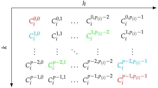
Figure 1.
Mutually antithetic strata are highlighted in the same color. These are domains and codomains of all , while the matrix itself represents . E.g. maps from to and vice versa, maps from to . For clarity, not all combinations are highlighted in color. We focus on and in red, and in blue and and in green.
Remark 7.
It is easy to see that the domains of the subfunctions from Remark 6 form a partition of the domain of , i.e., and for and . It is trivial that this is also true for the codomain of , i.e., the codomains of all are a partition of the codomain of . It is clear that the subfunctions from Remark 6 are bijective.
4.2. Computing Owen Values Using Antithetic Sampling
For the Owen value, we use the algorithm from [38] as the base algorithm. In each iteration, the algorithm chooses a random permutation of players for each precoalition with . Then, it chooses a random permutation of those precoalitions. This results in an order . The estimated Owen value is the average marginal contribution of player i to for all sampled orders , where returns the set of all players before player i for a given order as explained in Equation (5).
Compared to the base algorithm, in the antithetic variant the number of randomly taken samples is halved and for each of the remaining ⌈⌉ samples S an antithetic sample is generated via . Note that inside the description of Algorithm 8, the sampling procedure takes each permutation , i.e., each permutation compatible with the partition P, with the same probability. Concretely, it chooses a random permutation of the elements of each precoalition and then it takes at random a permutation of the p precoalitions.
Theorem 6.
The estimator for the Owen value of player i from Algorithm 8 is both unbiased, i.e., , and consistent, i.e., for all .
Proof.
The paper [38] shows that the estimator of the base algorithm is both unbiased and consistent. Again, the estimator is a sample mean while the true value is a population mean. Thus, we need to show that calling does not change this behavior, i.e., the resulting estimator in our algorithm is still a sample mean. To prove that, we need to show that the samples obtained by calling follow the same probability distribution as if they were directly randomly sampled. This means showing that maps every given subset to a unique antithetic subset that has an equal probability of being chosen during the random sampling process. For the Owen value, the probability of randomly sampling a subset S with k other precoalitions and h other players from player i’s precoalition is given by
whereby it is easy to see that a subset with a given k and h has an equal probability of being randomly sampled as a subset with other precoalitions and other players from player i’s own precoalition due to the symmetry of the binomial coefficients. This matches our definitions of all , where each maps a subset from to an antithetic subset from . Thus, the elements from the domain and codomain of all have an equal probability of being chosen during random sampling. Furthermore, we pointed out that these subfunctions are bijective, which means that each element of the domain maps to a unique element of the codomain and thus the elements of the codomain are i.i.d. among themselves. Therefore, the antithetic estimator of the Owen value is still a sample mean and hence both unbiased and consistent. □
| Algorithm 8 Antithetic sampling for Owen value approximation |
for do Take a random order , i.e., a permutation compatible with the partition P for do end for end for |
4.3. Computing Owen Values Using a Combination of Stratified and Antithetic Sampling
The article [29] presents a stratified sampling algorithm for the Owen value. The algorithm divides the population into strata based on the number of other precoalitions , denoted by , and on the number of players from , denoted by . The marginal contributions of player i in each of these strata are averaged and the estimator is the weighted sum over the averages of all strata. The strata weights are defined as
for the Owen value.
There are different possibilities of how an antithetic version of this algorithm can be implemented. We already proposed a stratified antithetic sampling algorithm for the Shapley value in Section 3.3 where the algorithm runs only for instead of for all because the strata of the positions can be reached through the antithetic sampling process. Based on that previous observation, an intuitive approach for the use with precoalitions would be to run only for and , whereas only samples from these strata are taken and all others samples for all other positions are generated via antithetic sampling. However, this leads to no samples being taken from strata where as well as . This problem is visualized in Figure 2.
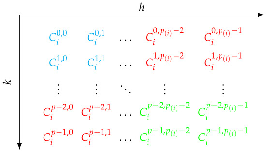
Figure 2.
It is not possible to reach all strata through antithetic sampling when running for and . Directly sampled strata are highlighted in blue, those generated through antithetic sampling in green, and those that cannot be reached in red.
Running either one of the variables or for or , respectively, are possible solutions to this problem. Both approaches result in reaching all combinations of k and h. We decided to run k for , which is visualized in Figure 3 and described in the following. Note that we employ the letter k again instead of , because we generally aim to use k as a loop variable for the precoalitions throughout this work whenever possible without creating ambiguity.

Figure 3.
When running for and , all strata can be reached. Directly sampled strata are highlighted in blue and those generated through antithetic sampling in green.
We commence by describing the algorithm for even . The algorithm becomes more complicated when is odd. We will go into more detail regarding the edge cases occurring for odd later.
For all and , a sample of size from stratum is taken and the corresponding antithetic sample from stratum is generated by calling for all . This leads to being also of size . Then, for all and the mean of marginal contributions of player i to all as well as is calculated, resulting in and , respectively. The estimator is the weighted sum over all those . The weights are defined in Equation (11). For these weights there holds , so that the same weight can be used for the estimators and .
While this idea works fine as long as is even, things become more complicated when is odd. In that case, there holds for , which means that samples with that value of and any given k are mapped to samples with the same and . Therefore, to avoid generating samples by both random sampling and the antithetic sample generation process, k is only allowed to be ran up to . This is visualized in Figure 4. Inside Algorithm 9, this is taken into account by calling continue to skip sampling subsets from strata with and .
| Algorithm 9 Stratified antithetic sampling for Owen value approximation |
for do for do if then continue end if for do Choose a random subset of size k Choose a random subset of size end for if ( then else end if end for end for |
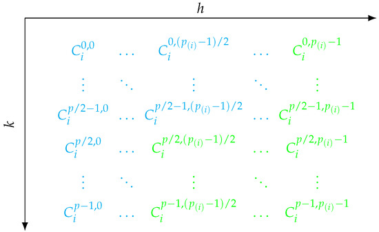
Figure 4.
If is odd and p is even, samples with are only taken from strata up to , i.e., those strata highlighted in blue in the middle column. Their corresponding antithetic samples are samples from the strata with the same amount of other players from player i’s precoalition and other precoalitions involved, i.e., those strata highlighted in green in the middle column. Note that directly sampled strata are highlighted in blue and those generated through antithetic sampling in green.
If, in addition to being odd, p is also odd, there is another effect that needs to be considered. In that case, there holds and for and . Thus, the estimators and are the same estimator. In that case, the estimator is updated twice per iteration and therefore uses samples. To correct that, the estimator will be divided by 2 before being added to the overall estimator , which is shown in the conditional statement at the end of the loop in Algorithm 9. We refer to Figure 5 for more details. The same edge case also needs to be taken into account if a proportional sample distribution over all strata is desired.
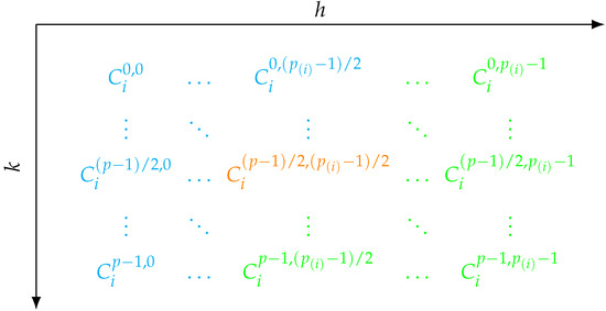
Figure 5.
If is odd and p is odd, the antithetic sample of the stratum is also from . This stratum is highlighted in orange, all other sampled strata are highlighted in blue, and the rest of the samples generated through antithetic sampling are highlighted in green.
We already showed that can alternatively be defined as multiple subfunctions . Taking a look at Equation (11), it is easy to see that the domain and the codomain of each are always equally weighted. Algorithm 10 creates a sample distribution that is proportional to the weights of the strata. For a total sample size m, the sample from the domain as well as the sample from the codomain of each can share the sample size , and thus the proportionality of the sample sizes with respect to the weights for all strata is still satisfied.
| Algorithm 10 Sample allocation for stratified antithetic sampling for Owen value approximation |
for do for do if then continue end if end for end for if then end if |
As we already mentioned, there is one edge case in which the sample size needs to be adapted if a proportional sample distribution is desired. If both p and are odd, then must be halved. This is due to the fact that a sample leads to a sample when using and for antithetic sample generation. When and , there holds and , which means that the antithetic sample generated via is once again taken from the same stratum as the input of , i.e., the domain and the codomain of are equal sets. This would result in sampling twice the sample size as specified in the variable . Hence, should be halved in advance as described in Algorithm 10.
Theorem 7.
The estimator for the Owen value of player i from Algorithm 9 with sample allocation according to Algorithm 10 is both unbiased, i.e., , and consistent, i.e., for all .
Proof.
The proof relies heavily on the study of stratified sampling for the Owen value in the paper by Saavedra-Nieves (2023) [29]. In [29], it is pointed out that the estimators associated with the strata are unbiased for all and all . The estimated Owen value is the mean over all those and hence unbiased as well. A proportional allocation procedure for all strata entails that implies for all strata and hence is consistent. Since our estimator can be interpreted as a weighted sum of means, we continue by showing that the estimator of each stratum is both unbiased and consistent.
In the following, we focus on the case that is even. For all strata with , the quantity is a sample mean and provides an unbiased estimator for which is a population mean of the underlying stratum. The samples of all other strata where are obtained by generating the antithetic samples from the strata that were directly sampled, i.e., for all , . We already showed that each is a bijection between its domain and its codomain. Thus, as long as the sample from the domain is i.i.d., the antithetic sample from the codomain is i.i.d. as well. Due to the random sampling process, it is given that the samples from the domains are i.i.d. and thus also the estimators with are sample means and therefore unbiased. It is clear that these arguments carry over to the case that is odd.
We pointed out that estimators for all strata are unbiased, which implies that the estimator as a weighted mean of those is also unbiased, i.e., . The sample allocation according to Algorithm 10 ensures that still guarantees for all strata and thus is consistent, i.e., for all . □
5. Results
In this section, we estimate Shapley, Banzhaf, and Owen values by using the algorithms proposed in this work. We use TU games for which the solution is known to measure the error. We employ the mean squared error (mse) defined as
for error measurement where is the estimator and E the true value, i.e., in practice E is replaced by for the Shapley value, by for the Banzhaf value, and by for the Owen value. We introduce our test games in Section 5.1 and then display, analyze, and interpret our computational results in Section 5.2.
5.1. Test Games with Known Solutions
In the following, we describe the four distinguished test games that are used throughout this section.
Airport Games go back to Littlechild and Thompson (1977) [45]. The problem consists of n players each owning an airplane that requires a specific runway length. The challenge that arises is how to divide the costs for a runway in a fashion that fits the needs of all players. This makes the airport problem into a special case of a maintenance problem in which the tree representing the problem turns out to be a line graph. For more details on airport games, including closed form solutions for the Shapley and Owen values, we refer to [46,47]. Let be an airport game with and v defined as
with cost vector .
We employ players in our tests for the Shapley values in Figure 6 and for the Banzhaf values in Figure 7. We note in passing that for players it is always possible to compute the exact solution (in an inefficient brute force manner) via the characteristic function v of the TU game, e.g. employing the R package CoopGame [48]. Concretely, we test airport games (13) with the cost vector
in Figure 6 for Shapley values and Figure 7 for Banzhaf values.
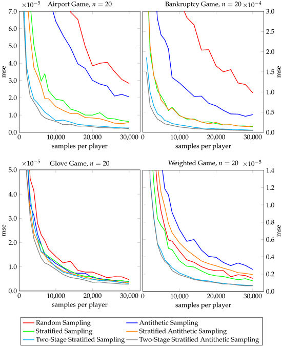
Figure 6.
Performance gain analysis of antithetic sampling for Shapley value estimation.
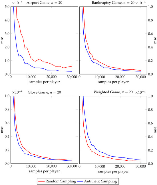
Figure 7.
Performance gain analysis of antithetic sampling for Banzhaf value estimation.
Furthermore, we always employ players in our tests for the Owen value. We always make use of the following precoalition structure
throughout this section. For our airport games with the precoalitions (15) and players, we simply duplicate the cost vector (14), i.e., we use . In Table 1, we also study Shapley values of airport games with low variance of the form
airport games with medium variance of the form
and airport games with high variance of the form

Table 1.
Execution times and MSEs for different antithetic sampling algorithms for approximating the Shapley value of four different airport games described in Section 5.1. The sample size per player is 30,000.
Bankruptcy games go back to O’Neill (1982) [49] who studied a problem of rights arbitration from the Talmud. Imagine a person dies leaving debts to n creditors. When the sum of the debts is greater than the value of the estate E of the deceased, we are confronted with the dilemma that the debts are mutually inconsistent because the estate is too small in order to meet all of the claims of the n creditors. We define a bankruptcy game v for a set of players , a debt vector c of length n, and an estate E as
Concretely, we use the claim vector c from (14) with estate for our bankruptcy games with players. In the case of the precoalitions (15) and players, we simply duplicate the claims vector (14), i.e., we use with estate .
Glove games are defined by a set of n players and a disjoint union with L being the set of players in possession of one left-hand glove each and R being the set of players in possession of one right-hand glove each. The worth of a coalition S is the number of pairs of gloves that the members of S can supply
For more details on glove games, we refer to the textbook by Peters (2015) [50], pp. 155–156. Concretely, for our glove games with players, the set of players with left-hand gloves is
and hence the set of players with right-hand gloves is . In the case of the precoalitions (15) and players, we work with
and .
Weighted games (also known as weighted voting games, weighted majority games, or quota games) have their origins in decision-making and voting in committees. Each player i from the player set is assigned a weight . A law or motion is passed in the voting body if the quota q is reached or exceeded, i.e.,
There are fast algorithms for computing point-valued solutions of weighted games. We refer to [51] for the exact algorithms and software we use for the Shapley and Banzhaf values and to [52,53] for solving weighted games with precoalitions. Despite these efficient methods for computing solutions exactly, weighted games also come out be very worthwhile test problems for Monte Carlo approximations. Concretely, we use the vector of weights with c from (14) and quota for our weighted games with players. In the case of the precoalitions (15) and players, we simply keep the idea of our quota as half the sum of all weights and duplicate our vector of weights (14), i.e., we use .
5.2. Numerical Results
We implemented our new algorithms introduced in Section 3 and Section 4 in R [54]. The implementations are part of an R package on Monte Carlo methods for cooperative games which is freely available via the github page of the first author at https://github.com/jhstaudacher/MonteCarloCooperativeGames/ (accessed on 4 October 2023).
All results were obtained under Microsoft Windows 10 Home (64-bit) on an Intel(R) Core(TM) i7-1165G7 CPU with a clock speed of 2.80 GHz and 16 GB RAM, i.e., on a standard laptop PC.
For our sampling algorithms, it is safe to assume that sampling the characteristic function (of the TU game to be approximated) is the most costly part of the computation. Hence, we always plot the number of samples per player (x-axis) against the mean squared error (mse, y-axis) (12).
Let us look at Figure 6 for the Shapley values first. For the airport, bankruptcy, and glove games, antithetic sampling (Algorithm 1) clearly outperforms classical random sampling. For the airport game, stratified antithetic sampling (Algorithm 2) performs better than stratified sampling, while it is safe to say that for the bankruptcy game and the glove game, stratified antithetic sampling does not do worse than stratified sampling. Also, for the airport, bankruptcy, and glove games, two-stage stratified antithetic sampling (Algorithm 6) never shows a worse performance than two-stage stratified sampling (Algorithm 4). However, for the weighted game the picture changes. Stratified antithetic sampling performs worse than stratified sampling and even loses to classical random sampling while antithetic sampling (without stratification) converges most slowly. Only two-stage antithetic stratified sampling performs equally well as its baseline counterpart for the weighted game. We study approximations of the Banzhaf value in Figure 7. For the airport, bankruptcy, and glove games, antithetic sampling (Algorithm 7) leads to faster convergence than classical random sampling in all three cases. Again, for the weighted game the observation is reversed as classical random sampling outperforms antithetic sampling.
We next turn our attention to the Owen value and Figure 8. For both the airport game and the bankruptcy game, antithetic sampling (Algorithm 8) clearly outperforms classical random sampling and stratified antithetic sampling (Algorithm 9) converges faster than stratified sampling. For the glove game, antithetic sampling still beats the base algorithm slightly, whereas stratified antithetic sampling and stratified sampling perform equally well. Again, for the weighted game our observations are different. The two antithetic variants converge more slowly than the base algorithms.
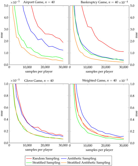
Figure 8.
Performance gain analysis of antithetic sampling for Owen value estimation.
We finally compare execution times and MSEs for Shapley value approximations for larger airport games with 40, 60, 80, and 100 players and 30000 samples per player in Table 1. As for the execution times, the authors are very well aware how these depend on their concrete implementation in R. Random antithetic sampling (Algorithm 1) always takes a little more time than random sampling (ApproShapley) and so does two-stage stratified antithetic sampling (Algorithm 6) as compared to two-stage stratified sampling (Algorithm 4). On the other hand, our stratified antithetic sampling approach (Algorithm 2) always needs slightly less computing time than stratified sampling (St-ApproShapley). In terms of the MSEs (which we deem much more meaningful and important than our execution times), the picture in Table 1 is very clear. Stratification in both its classical and our antithetic variant pays off in all four test cases when compared to approaches without stratification. Two-stage stratification in both its classical and our antithetic variant performs even better.
5.3. Comparison with the Ergodic Sampling Approach by Illés and Kerényi
Illés and Kerényi (2022) [55] propose ergodic sampling for approximating Shapley values, i.e., their sampled permutations are ergodic (meaning they follow the strong law of large numbers) but not independent. Ergodic sampling aims to construct pairs of negatively correlated samples in order to reduce the variance of the estimate implying that antithetic sampling can be regarded as the simplest heuristic for creating ergodic samples. Illés and Kerényi [55] propose a sophisticated algorithm to learn the best ergodic transform for a TU game at hand. Their algorithm consists of two stages. In the first stage , random permutations are sampled in order to learn an optimal ergodic transform t for a specific TU game via a greedy approach. In the second stage, this transform t is employed for actual ergodic rather than independent sampling, see [55] for a detailed description of the algorithms. Illés and Kerényi [55] provide a MATLAB implementation of their approach via https://de.mathworks.com/matlabcentral/fileexchange/71822-estimation-of-the-shapley-value-by-ergodic-sampling (accessed on 4 October 2023).
We ported their algorithm to R and integrated it into the package mentioned at the beginning of Section 5.2.
Table 2 compares our antithetic approaches and ergodic sampling with six different values of for a bankruptcy game with players. For all values of except for , ergodic sampling leads to a lower MSE than random sampling (ApproShapley), but it is outperformed by random antithetic sampling (Algorithm 1). All the four stratified sampling approaches lead to superior results.
Table 2.
Execution times and MSEs for different antithetic sampling algorithms and ergodic sampling for approximating the Shapley value of the bankruptcy game described in Section 5.1, i.e., a bankruptcy game with players, the claims vector defined in Equation (14), and estate . The sample size per player is 100,000, which means the overall sample size is m = 2,000,000.
5.4. Critical Appraisal of Antithetic Sampling
On the one hand, our experiments confirm that the concept of antithetic sampling bears plenty of promise for accelerating estimations of Shapley, Banzhaf, and Owen values. On the other hand, we observe that this concept cannot be recommended unconditionally. From a very broad perspective, our experiments affirm in the context of permutation sampling for TU games that “stratification” is a much more powerful concept for variance reduction than “incorporating antithetic samples into an established algorithm”.
The question whether antithetic sampling algorithms truly lead to acceleration appears to depend on the game at hand, its properties, and its parametrization. For example, we observe that both airport games and bankruptcy games are convex games, whereas glove games and weighted games are not convex in general. A TU game v is called convex if for all , see [2], p. 10. Our experiments show that antithetic sampling can lead to an increase rather than a decrease in variance, a phenomenon Illés and Kerényi [55] also observe for ergodic sampling in some examples in their paper.
Finally, there is clearly a lack of analytical understanding of antithetic sampling in the context of estimating Shapley values. As long as we are unable to estimate the decrease in variance achieved via antithetic sampling, we will not be able to quantify the sample size a practitioner needs in order to guarantee a certain theoretical error. In such a case, one could only rely on the error bound for the base variant (rather than the antithetic variant) of the algorithm. For example, for the classical ApproShapley algorithm, we could still rely on bounds for the estimation error based on Hoeffding’s inequality from the paper by Maleki et al. (2013) [42] in cases where the variance of marginal contributions or the range of marginal contributions is known. We agree with the remarks by Illés and Kerényi [55] that it is not known how to quantify the quality of variance reduction methods for the Shapley value as one can find only illustrative examples, but no statistical results, on this question in the literature.
6. Conclusions
This article studies antithetic permutation sampling for approximating three point-valued solution concepts from cooperative game theory, i.e., the Shapley, Banzhaf, and Owen values. We provide a detailed analysis of antithetic subset generation and present novel antithetic sampling algorithms for the Banzhaf and Owen values. We show how to combine stratified sampling and antithetic sampling and develop sophisticated algorithms for the Shapley and Owen values. We point out that all our estimators are both unbiased and consistent.
This study was motivated by the widespread usage of antithetic sampling approximations of Shapley values in interpretable machine learning [18,20,23] which employ randomly sampled permutations together with their reverse permutations. The goal of our research was to provide a detailed assessment of the potential of antithetic sampling in the context of sampling permutations or subsets. Deliberately, we did not only study Shapley values, but also the Banzhaf and Owen values in order to ensure that our observations are also valid for other solution concepts based on marginal contributions and in the presence of precoalitions.
Our numerical experiments support the assessment that the concept of antithetic variates can lead to faster convergence of sampling algorithms for Shapley, Banzhaf, and Owen values, especially when combined with existing approaches for stratified sampling. However, we also find that this is not always the case and hence antithetic sampling should not be recommended without reservation. We regret the lack of theoretical bounds for the estimation error for antithetic sampling as compared to their corresponding base methods employing i.i.d. sampling. Our experiments show that stratification has a more profound effect on improving Shapley value estimations than our additional incorporation of antithetic sampling.
We wish to emphasize that this article is definitely not meant to be an overview of state-of-the-art algorithms for estimating Shapley values. Our subject is limited to antithetic sampling with replacement. While our paper reports very favorable results for Neyman sampling, i.e., the two-stage stratified sampling algorithm from [22], we need to stress that we omitted other important stratification methods, in particular Bernstein sampling introduced by Burgess and Chapman in their papers [31,32]. We are certain it would not have changed our evaluation of antithetic sampling. Also, we deliberately did not include sampling approaches without replacement [31,32] in this study. While these approaches allow for sharper error bounds, they are more sophisticated to implement and discuss as storage requirements might become more critical. We are convinced that incorporating antithetic samples into existing algorithms without replacement in a similar fashion to our study would not lead to a different assessment of the advantages and disadvantages of antithetic sampling.
Finally, our research emphasizes an open research question already posed similarly by Illés and Kerényi [55]. Can we identify classes of TU games for which specific Monte Carlo methods perform well? Can we identify certain favorable properties of TU games in the latter context, ideally independent from the parametrization of the games? Trying to build upon the work by Liben-Nowell et al. (2012) [30] could provide a starting point.
Author Contributions
Conceptualization, J.S. and T.P.; Methodology, J.S. and T.P.; Software, T.P.; Validation, J.S.; Formal Analysis, J.S. and T.P.; Writing—original draft, J.S. and T.P.; Writing—review & editing, J.S. and T.P. All authors have read and agreed to the published version of the manuscript.
Funding
This research received no external funding.
Institutional Review Board Statement
Not applicable.
Informed Consent Statement
Not applicable.
Data Availability Statement
Data are contained within the article.
Acknowledgments
The first authors thanks the partial funding of the Bavarian Ministry of Science and Arts. Both authors thank three anonymous reviewers for their careful reading of the paper and their valuable comments.
Conflicts of Interest
The authors declare no conflict of interest.
References
- Branzei, R.; Dimitrov, D.; Tijs, S. Models in Cooperative Game Theory; Springer: Berlin/Heidelberg, Germany, 2008. [Google Scholar] [CrossRef]
- Peleg, B.; Sudhölter, P. Introduction to the Theory of Cooperative Games, 2nd ed.; Springer: Berlin/Heidelberg, Germany, 2007. [Google Scholar] [CrossRef]
- Algaba, E.; Bilbao, J.M.; Fernández-García, J.R. The distribution of power in the European Constitution. Eur. J. Oper. Res. 2007, 176, 1752–1766. [Google Scholar] [CrossRef]
- Kóczy, L.A. Beyond Lisbon. Demographic trends and voting power in the European Union Council of Ministers. Math. Soc. Sci. 2012, 63, 152–158. [Google Scholar] [CrossRef]
- Kóczy, L.A. Brexit and Power in the Council of the European Union. Games 2021, 12, 51. [Google Scholar] [CrossRef]
- Moretti, S.; Patrone, F.; Bonassi, S. The class of microarray games and the relevance index for genes. Top 2007, 15, 256–280. [Google Scholar] [CrossRef]
- Lucchetti, R.; Radrizzani, P. Microarray Data Analysis via Weighted Indices and Weighted Majority Games. In Computational Intelligence Methods for Bioinformatics and Biostatistics. CIBB 2009. Lecture Notes in Computer Science; Masulli, F., Peterson, L.E., Tagliaferri, R., Eds.; Springer: Berlin/Heidelberg, Germany, 2009; Volume 6160, pp. 179–190. [Google Scholar] [CrossRef]
- Algaba, E.; Prieto, A.; Saavedra-Nieves, A.; Hamers, H. Analyzing the Zerkani Network with the Owen Value. In Advances in Collective Decision Making. Studies in Choice and Welfare; Kurz, S., Maaser, N., Mayer, A., Eds.; Springer: Cham, Switzerland, 2023. [Google Scholar] [CrossRef]
- Algaba, E.; Prieto, A.; Saavedra-Nieves, A. Risk analysis sampling methods in terrorist networks based on the Banzhaf value. Risk Anal. 2023, 1–16. [Google Scholar] [CrossRef] [PubMed]
- van Campen, T.; Hamers, H.; Husslage, B.; Lindelauf, R. A new approximation method for the Shapley value applied to the WTC 9/11 terrorist attack. Soc. Netw. Anal. Min. 2018, 8, 3. [Google Scholar] [CrossRef]
- Staudacher, J.; Olsson, L.; Stach, I. Implicit power indices for measuring indirect control in corporate structures. In Transactions on Computational Collective Intelligence XXXVI. Lecture Notes in Computer Science; Nguyen, N., Kowalczyk, R., Mercik, J., Motylska-Kuźma, A., Eds.; Springer: Berlin/Heidelberg, Germany, 2021; Volume 13010, pp. 73–93. [Google Scholar] [CrossRef]
- Staudacher, J.; Olsson, L.; Stach, I. Algorithms for measuring indirect control in corporate networks and effects of divestment. In Transactions on Computational Collective Intelligence XXXVII, Lecture Notes in Computer Science; Nguyen, N.T., Kowalczyk, R., Mercik, J., Motylska-Kuźma, A., Eds.; Springer: Berlin/Heidelberg, Germany, 2022; Volume 13750, pp. 53–74. [Google Scholar] [CrossRef]
- Shapley, L.S. A value for n-person games. Contrib. Theory Games 1953, 28, 307–317. [Google Scholar]
- Fernández, J.R.; Algaba, E.; Bilbao, J.M.; Jiménez, A.; Jiménez, N.; López, J.J. Generating functions for computing the Myerson value. Ann. Oper. Res. 2002, 9, 143–158. [Google Scholar] [CrossRef]
- Deng, X.; Papadimitriou, C.H. On the complexity of cooperative solution concepts. Math. Oper. Res. 1994, 19, 257–266. [Google Scholar] [CrossRef]
- Faigle, U.; Kern, W. The Shapley value for cooperative games under precedence constraints. Int. J. Game Theory 1992, 21, 249–266. [Google Scholar] [CrossRef]
- Rozemberczki, B.; Watson, L.; Bayer, P.; Yang, H.; Kiss, O.; Nilsson, S.; Sarkar, R. The Shapley value in machine learning. In Proceedings of the 31st International Joint Conference on Artificial Intelligence, Vienna, Austria, 23–29 July 2022; de Raedt, L., Ed.; International Joint Conferences on Artificial Intelligence Organization: Vienna, Austria, 2022; pp. 5572–5579. [Google Scholar] [CrossRef]
- Chen, H.; Covert, I.C.; Lundberg, S.M.; Lee, S. Algorithms to estimate Shapley value feature attributions. Nat. Mach. Intell. 2023, 5, 590–601. [Google Scholar] [CrossRef]
- Lundberg, S.M.; Lee, S. A unified approach to interpreting model predictions. Adv. Neural Inf. Process. Syst. 2017, 30, 4768–4777. [Google Scholar]
- Molnar, C. Interpreting Machine Learning Models with SHAP; LeanPub: Victoria, BC, Canada, 2023; Available online: https://leanpub.com/shap (accessed on 4 October 2023).
- Castro, J.; Gómez, D.; Tejada, J. Polynomial calculation of the Shapley value based on sampling. Comput. Oper. Res. 2009, 36, 1726–1730. [Google Scholar] [CrossRef]
- Castro, J.; Gómez, D.; Molina, E.; Tejada, J. Improving polynomial estimation of the Shapley value by stratified random sampling with optimum allocation. Comput. Oper. Res. 2017, 82, 180–188. [Google Scholar] [CrossRef]
- Mitchell, R.; Cooper, J.; Frank, E.; Holmes, G. Sampling permutations for Shapley value estimation. J. Mach. Learn. Res. 2022, 23, 2082–2127. Available online: http://jmlr.org/papers/v23/21-0439.html (accessed on 4 October 2023).
- Ballester-Ripoll, R. Tensor approximation of cooperative games and their semivalues. Int. J. Approx. Reason. 2022, 142, 94–108. [Google Scholar] [CrossRef]
- Banzhaf, J.F., III. Weighted voting doesn’t work: A mathematical analysis. Rutgers L. Rev. 1964, 19, 317. [Google Scholar]
- Owen, G. Multilinear extensions and the Banzhaf value. Nav. Res. Logist. Q. 1975, 22, 741–750. [Google Scholar] [CrossRef]
- Wang, J.T.; Jia, R. DataBanzhaf: A robust data valuation framework for machine learning. In Proceedings of the International Conference on Artificial Intelligence and Statistics, Valencia, Spain, 25–27 April 2023; Camps-Valls, G., Ruiz, F., Valera, I., Eds.; PMLR: London, UK, 2023; Volume 151, pp. 6388–6421. Available online: https://proceedings.mlr.press/v206/wang23e/wang23e.pdf (accessed on 4 October 2023).
- Owen, G. Values of Games with a Priori Unions. In Mathematical Economics and Game Theory. Lecture Notes in Economics and Mathematical Systems; Henn, R., Moeschlin, O., Eds.; Springer: Berlin/Heidelberg, Germany, 1977; Volume 141, pp. 76–88. [Google Scholar] [CrossRef]
- Saavedra-Nieves, A. On stratified sampling for estimating coalitional values. Ann. Oper. Res. 2023, 320, 325–353. [Google Scholar] [CrossRef]
- Liben-Nowell, D.; Sharp, A.; Wexler, T.; Woods, K. Computing shapley value in supermodular coalitional games. In Computing and Combinatorics. COCOON 2012. Lecture Notes in Computer Science; Gudmundsson, J., Mestre, J., Viglas, T., Eds.; Springer: Berlin/Heidelberg, Germany, 2012; Volume 7434, pp. 568–579. [Google Scholar] [CrossRef]
- Burgess, M.A.; Chapman, A.C. Stratied Finite Empirical Bernstein Sampling. Preprints 2019, 1–30. [Google Scholar] [CrossRef]
- Burgess, M.A.; Chapman, A.C. Approximating the Shapley Value Using Stratified Empirical Bernstein Sampling. In Proceedings of the IJCAI, Montreal, QC, Canada, 19–27 August 2021; pp. 73–81. [Google Scholar]
- Owen, G. Multilinear extensions of games. Manag. Sci. 1972, 18, 64–79. [Google Scholar] [CrossRef]
- Okhrati, R.; Lipani, A. A Multilinear Sampling Algorithm to Estimate Shapley Values. In Proceedings of the 2020 25th International Conference on Pattern Recognition (ICPR), Milan, Italy, 10–15 January 2021; pp. 7992–7999. [Google Scholar] [CrossRef]
- Soufiani, H.A.; Charles, D.X.; Chickering, D.M.; Parkes, D.C. Approximating the shapley value via multi-issue decomposition. In Proceedings of the International Foundation for Autonomous Agents and Multiagent Systems, Paris, France, 5–9 May 2014; pp. 1209–1216. [Google Scholar]
- Corder, K.; Decker, K. Shapley value approximation with divisive clustering. In Proceedings of the 18th IEEE International Conference on Machine Learning and Applications (ICMLA), Boca Raton, FL, USA, 16–19 December 2019; pp. 234–239. [Google Scholar] [CrossRef]
- Jethani, N.; Sudarsan, M.; Covert, I.C.; Lee, S. Fastshap: Real-time shapley value estimation. In Proceedings of the International Conference on Learning Representations, Virtual, 3–7 May 2021. [Google Scholar]
- Saavedra-Nieves, A.; García-Jurado, I.; Fiestras-Janeiro, M.G. Estimation of the Owen value based on sampling. In The Mathematics of the Uncertain: A Tribute to Pedro Gil. Studies in Systems, Decision and Control; Gil, E., Gil, E., Gil, J., Gil, M., Eds.; Springer: Cham, Switzerland, 2018; Volume 142, pp. 347–356. [Google Scholar] [CrossRef]
- Botev, Z.; Ridder, A. Variance reduction. In Wiley statsRef: Statistics Reference Online; Wiley: Hoboken, NJ, USA, 2017; pp. 1–6. [Google Scholar] [CrossRef]
- Rubinstein, R.; Kroese, D. Monte Carlo methods. Wiley Interdiscip. Rev. Comput. Stat. 2012, 4, 48–58. [Google Scholar] [CrossRef]
- Lomeli, M.; Rowland, M.; Gretton, A.; Ghahramani, Z. Antithetic and Monte Carlo kernel estimators for partial rankings. Stat. Comput. 2019, 29, 1127–1147. [Google Scholar] [CrossRef]
- Maleki, S.; Tran-Thanh, L.; Hines, G.; Rahwan, T.; Rogers, A. Bounding the estimation error of sampling-based Shapley value approximation. arXiv 2013, arXiv:1306.4265. [Google Scholar]
- Neyman, J. On the Two Different Aspects of the Representative Method: The Method of Stratified Sampling and the Method of Purposive Selection. J. R. Stat. 1934, 97, 558–625. [Google Scholar] [CrossRef]
- Saavedra-Nieves, A. Statistics and game theory: Estimating coalitional values in R software. Oper. Res. Lett. 2021, 49, 129–135. [Google Scholar] [CrossRef]
- Littlechild, S.C.; Thompson, G.F. Aircraft landing fees: A game theory approach. Bell J. Econ. 1977, 8, 186–204. [Google Scholar] [CrossRef]
- Borm, P.; Hamers, H.; Hendrickx, R. Operations research games: A survey. Top 2001, 9, 139–199. [Google Scholar] [CrossRef]
- Vázquez-Brage, M.; van den Nouweland, A.; García-Jurado, I. Owen’s coalitional value and aircraft landing fees. Math. Soc. Sci. 1997, 34, 273–286. [Google Scholar] [CrossRef]
- Staudacher, J.; Anwander, J. Using the R Package CoopGame for the Analysis, Solution and Visualization of Cooperative Games with Transferable Utility. R Vignette for Package Version 0.2.2. 2021. Available online: https://cran.r-project.org/package=CoopGame (accessed on 20 October 2023).
- O’Neill, B. A problem of rights arbitration from the Talmud. Math. Soc. Sci. 1982, 2, 345–371. [Google Scholar] [CrossRef]
- Peters, H. Game Theory: A Multi-Leveled Approach, 2nd ed.; Springer: Berlin/Heidelberg, Germany, 2015. [Google Scholar] [CrossRef]
- Staudacher, J.; Kóczy, L.Á.; Stach, I.; Filipp, J.; Kramer, M.; Noffke, T.; Olsson, L.; Pichler, J.; Singer, T. Computing power indices for weighted voting games via dynamic programming. Oper. Res. Dec. 2021, 31, 123–145. [Google Scholar] [CrossRef]
- Staudacher, J.; Wagner, F.; Filipp, J. Dynamic Programming for Computing Power Indices for Weighted Voting Games with Precoalitions. Games 2021, 13, 6. [Google Scholar] [CrossRef]
- Staudacher, J. Computing the Public Good index for weighted voting games with precoalitions using dynamic programming. In Power and Responsibility: Interdisciplinary Perspectives for the 21st Century in Honor of Manfred J. Holler; Leroch, M.A., Rupp, F., Eds.; Springer: Cham, Switzerland, 2023; pp. 107–124. [Google Scholar] [CrossRef]
- R Core Team, R. A Language and Environment for Statistical Computing; R Foundation for Statistical Computing: Vienna, Austria, 2023; Available online: https://www.R-project.org/ (accessed on 4 October 2023).
- Illés, F.; Kerényi, P. Estimation of the Shapley value by ergodic sampling. arXiv 2022, arXiv:1906.05224v2. [Google Scholar]
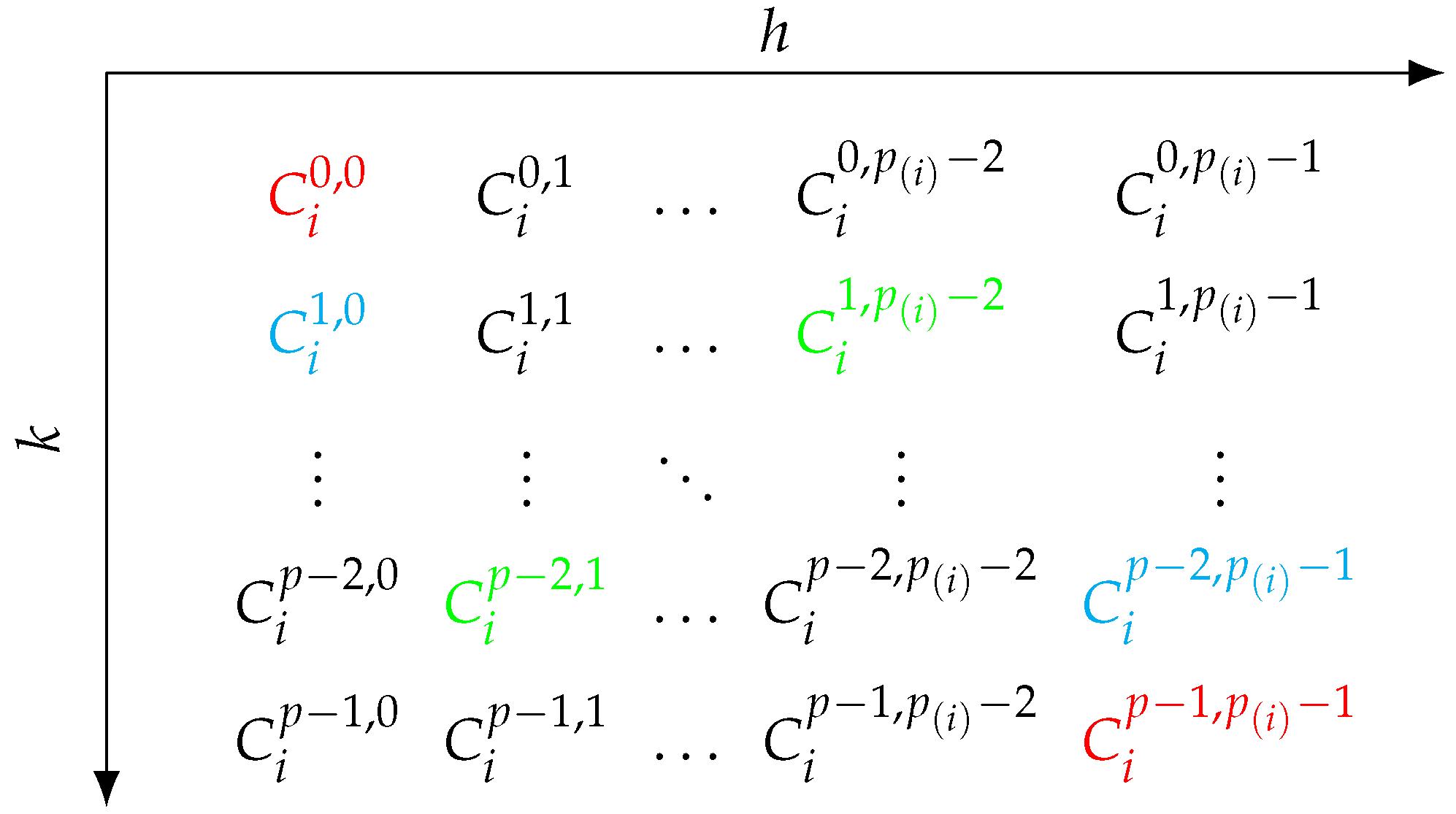

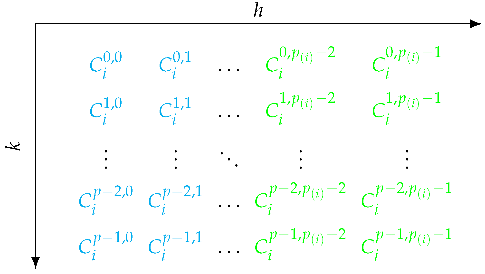
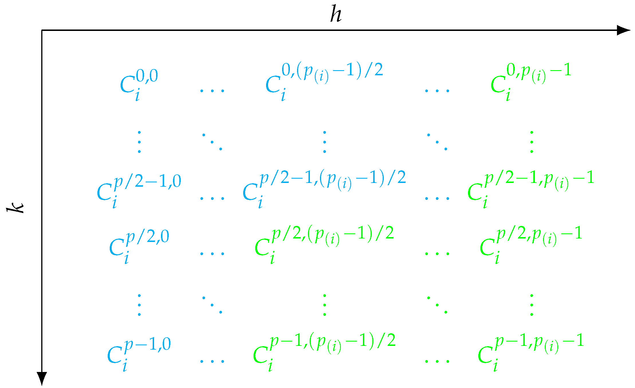

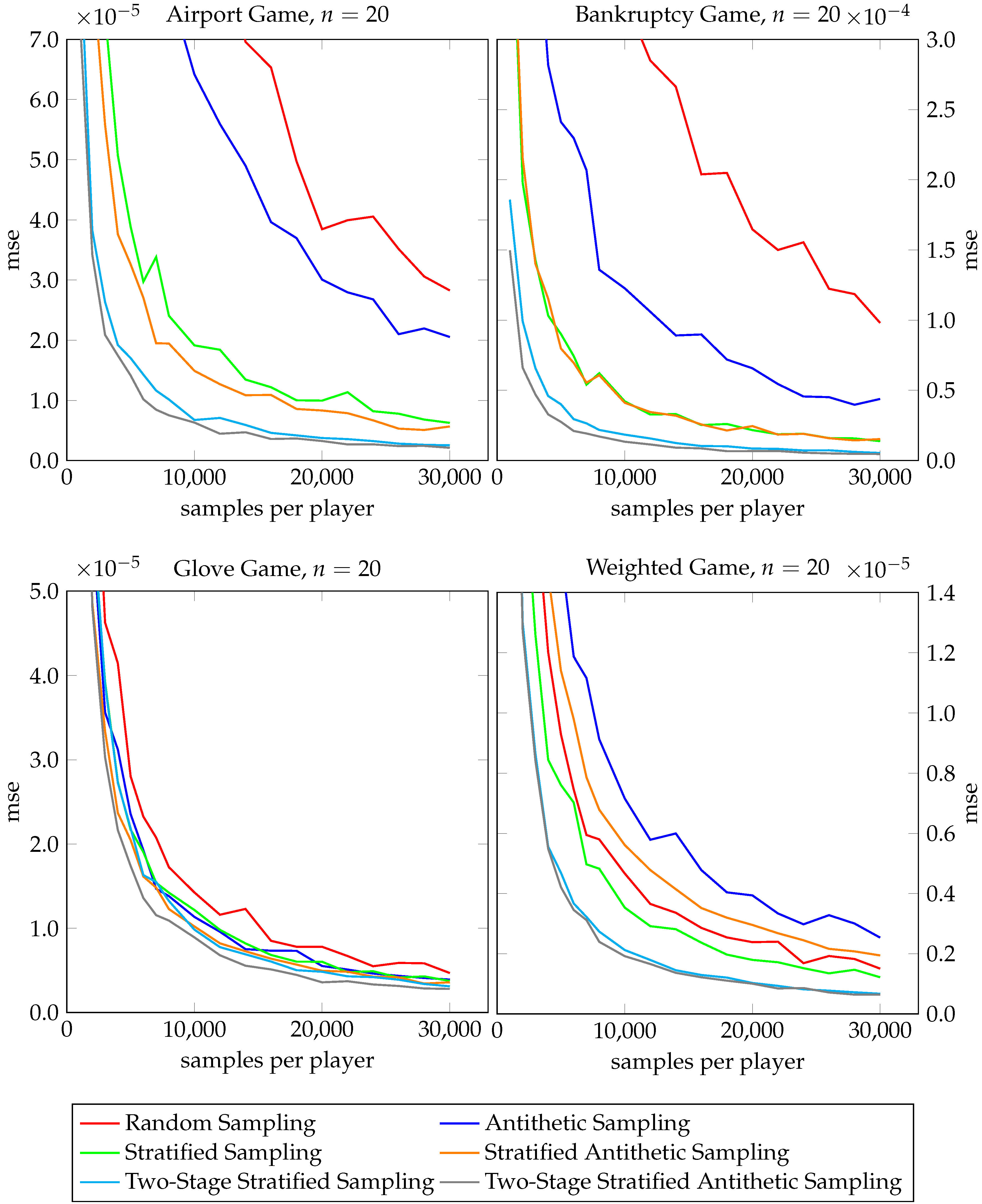
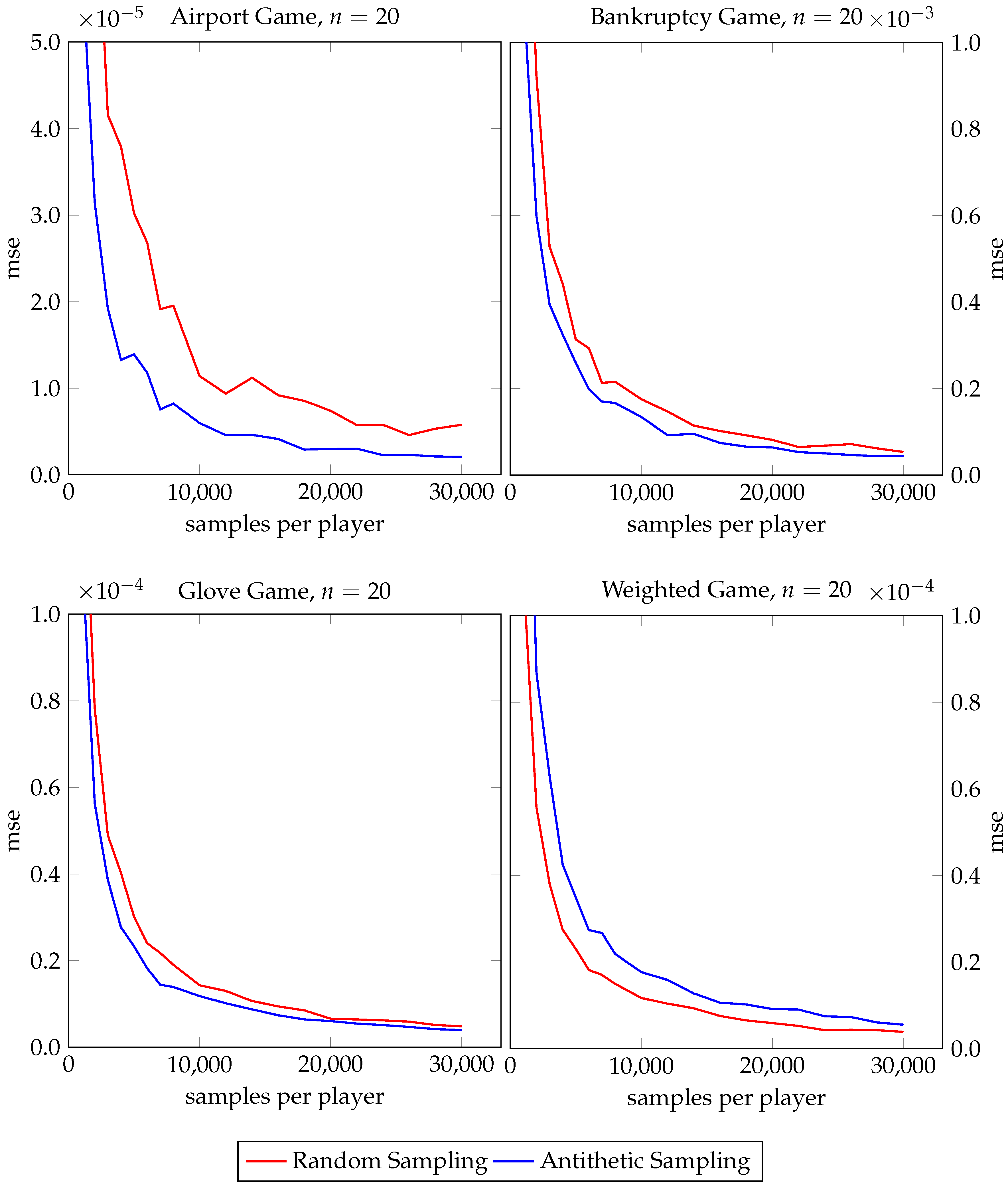
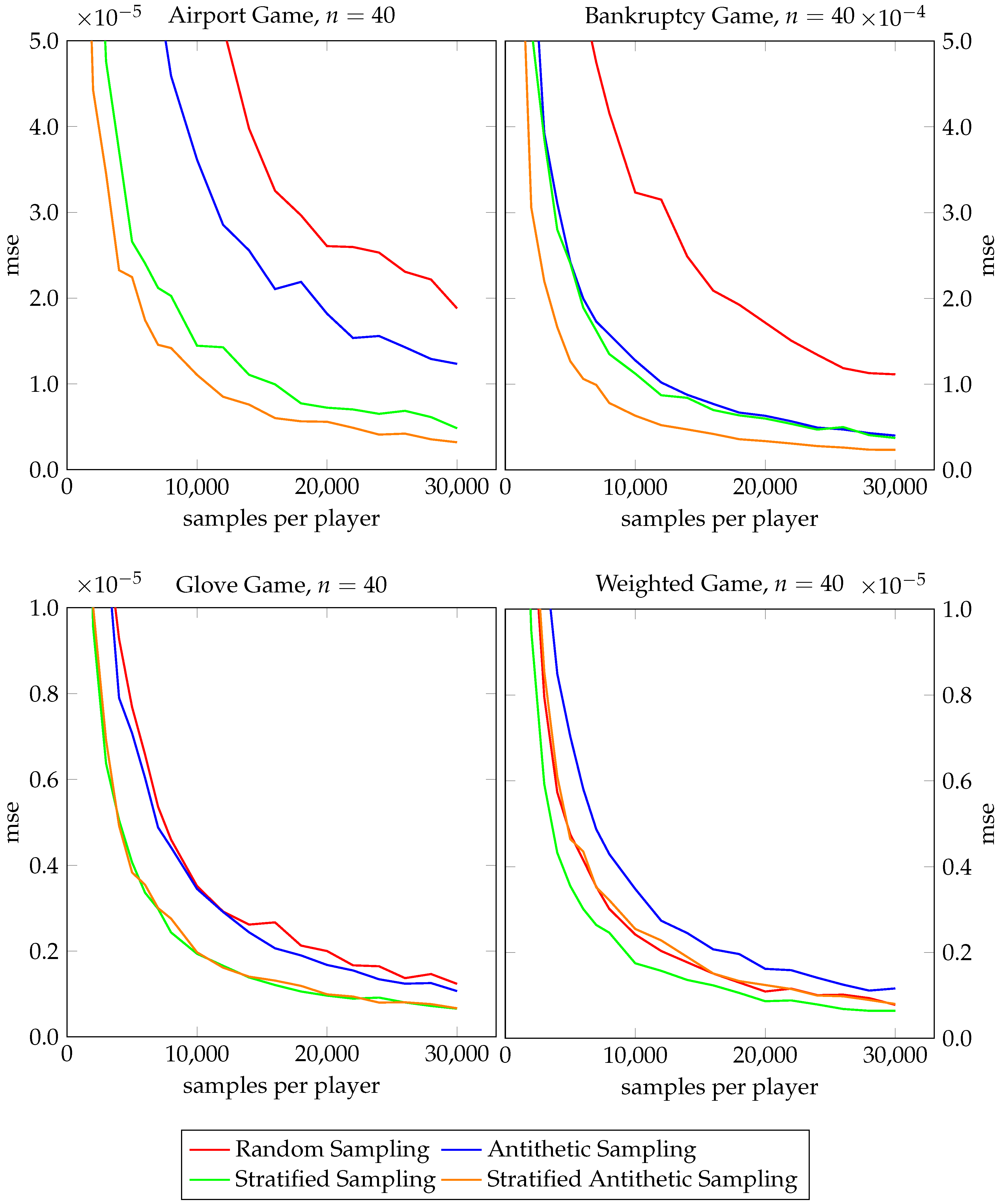
Disclaimer/Publisher’s Note: The statements, opinions and data contained in all publications are solely those of the individual author(s) and contributor(s) and not of MDPI and/or the editor(s). MDPI and/or the editor(s) disclaim responsibility for any injury to people or property resulting from any ideas, methods, instructions or products referred to in the content. |
© 2023 by the authors. Licensee MDPI, Basel, Switzerland. This article is an open access article distributed under the terms and conditions of the Creative Commons Attribution (CC BY) license (https://creativecommons.org/licenses/by/4.0/).