Mathematical Formalism and Physical Models for Generative Artificial Intelligence

Abstract

This paper presents a mathematical formalism for generative artificial intelligence (GAI). Our starting point is an observation that a “histories” approach to physical systems agrees with the compositional nature of deep neural networks. Mathematically, we define a GAI system as a family of sequential joint probabilities associated with input texts and temporal sequences of tokens (as physical event histories). From a physical perspective on modern chips, we then construct physical models realizing GAI systems as open quantum systems. Finally, as an illustration, we construct physical models realizing large language models based on a transformer architecture as open quantum systems in the Fock space over the Hilbert space of tokens. Our physical models underlie the transformer architecture for large language models.

1. Introduction

Generative artificial intelligence (AI) models are important for modeling intelligent machines as physically described in [1,2]. Generative AI is based on deep neural networks (DNNs for short), and a common characteristic of DNNs is their compositional nature (cf. [3]): data is processed sequentially, layer by layer, resulting in a discrete-time dynamical system. The introduction of the transformer architecture for generative AI in 2017 marked the most striking advancement in terms of DNNs (cf. [4]). Indeed, the transformer is a model architecture eschewing recurrence and instead relying entirely on an attention mechanism to draw global dependencies between input and output. At each step, the model is auto-regressive, consuming the previously generated symbols as additional input when generating the next. The transformer has achieved great success in natural language processing (cf. [5]).

The transformer has a modularization framework and is constructed by two main building blocks: self-attention and feed-forward neural networks. Self-attention is an attention mechanism relating different positions of a single sequence in order to compute a representation of the sequence. However, despite its meteoric rise within deep learning, we believe there is a gap in our theoretical understanding of what the transformer is and why it works physically (cf. [6]).

We think that there are two origins for the modularization framework of generative AI models. One is a mathematical origin in which a joint probability distribution can be computed by sequentially conditional probabilities. For instance, the probability of generating a text $t_1{t}_2\cdots t_N$ given an input X in a transformer architecture is equal to the joint probability distribution $P_X(t_1,\cdots ,t_N)$ such that

$$P_X(t_1,\cdots ,t_N)=P_X(t_1)P_X(t_2|t_1)\cdots P_X(t_N|t_1,\dots ,t_{N-1}),$$

(1)

where the conditional probability $P_X(t_{\ell }|t_1,\dots ,t_{\ell -1})$ is given by the ℓ-th attention block in the transformer. Another is a physical origin, in which a physical process is considered to be a sequence of events as a history. As such, generating a text $t_1{t}_2\cdots t_N$ given an input X in a physical machine is a process in which, given an input X at time ${\tau }_0,$ an event $|t_1⟩⟨t_1|$ occurs at time ${\tau }_1,$ an event $|t_2⟩⟨t_2|$ occurs at time ${\tau }_2,$ …, and last, an event $|t_N⟩⟨t_N|$ occurs at time ${\tau }_N$. A theory of the “histories” approach to physical systems was established by Isham [2], and the mathematical theory of it associated with joint probability distributions was then developed by Gudder [1]. Based on their theory, in this paper, we present a mathematical formalism for generative AI and describe the associated physical models.

To the best of our knowledge, physical models for generative AI are usually described by using systems of mean-field interacting particles (cf. [7,8] and references therein); i.e., generative AI models are regarded as classical statistical systems. However, since modern chips process data by controlling the flow of electric current, i.e., the dynamics of many electrons, they should be regarded as quantum statistical ensembles and open quantum systems from a physical perspective (cf. [9,10]). Consequently, based on our mathematical formalism for generative AI, we construct physical models realizing generative AI systems as open quantum systems. As an illustration, we construct physical models realizing large language models based on a transformer architecture as open quantum systems in the Fock space over the Hilbert space of tokens.

The paper is organized as follows. In Section 2, we include some notation and definitions on the attention mechanism, the transformer, and the effect algebras. In Section 3, we give the definition of a generative AI system as a family of sequential joint probabilities associated with input texts and temporal sequences of tokens. This is based on the mathematical theory developed by Gudder (cf. [1]) for a historical approach to physical evolution processes. Those joint probabilities characterize the attention mechanisms as well as the mathematical structure of the transformer architecture. In Section 4, we present the construction of physical models realizing generative AI systems as open quantum systems. Our physical models are given by an event-history approach to physical systems; we refer to [2] for the background of physics for this formulation. In Section 5, we construct physical models realizing large language models based on a transformer architecture as open quantum systems in the Fock space over the Hilbert space of tokens. Finally, in Section 6, we give a summary of our innovative points listed item by item and conclude the contributions of the paper.

2. Preliminaries

In this section, we present a mathematical description of the attention mechanism and transformer architecture for generative AI and include some notations and basic properties of $\sigma$-effect algebras (cf. [11]). For the sake of convenience, we collect some notations and definitions. Denote by $\mathbb{N}$ the natural number set $\{1,2,\cdots \},$ and for $n\in \mathbb{N},$ we use the notation $\left[n\right]$ to represent the set $\{1,\dots ,n\}.$ For $d\in \mathbb{N},$ we denote by ${\mathbb{R}}^d$ the d-dimensional Euclid space with the usual inner product $⟨-,-⟩.$ For two sets $X,Y,$ we denote by $\mathrm{Hom}(X,Y)$ the set of all maps from X into $Y.$ For a set $S,$ we denote $S^{*}={\bigcup }_{n\in \mathbb{N}}{S}^{(n)},$ where $S^{(n)}$ is the set of all sequences $(s_1,\dots ,s_n)$ of n elements in S; i.e., $S^{*}$ is the set of all finite sequences of elements in $S.$

2.1. Deep Neural Networks

A DNN is constructed by connecting multiple neurons. Recall that a (feed-forward) neural network of depth L consists of some number of neurons arranged in $L+1$ layers. Layer $\ell =0$ is the input layer, where data is presented to the network, while layer $\ell =L$ is where the output is read out. All layers in between are referred to as the hidden layers, and each hidden layer has an activation that is a map in the same layer. Specifically, let ${\left\{X_{\ell }\right\}}_{\ell =0}^L$ be a sequence of sets where $X_{\ell }$ indexes the neurons in layer $\ell ,$ and let ${\left\{V_{\ell }\right\}}_{\ell =0}^L$ be a sequence of vector spaces. A mapping $\mathsf{\Phi }:\mathrm{Hom}(X_0,V_0)\mapsto \mathrm{Hom}(X_L,V_L)$ is called a feed-forward neural network of depth L if there exists a sequence ${\left\{W_{\ell }\right\}}_{\ell =1}^L$ of maps $W_{\ell }:\mathrm{Hom}(X_{\ell -1},V_{\ell -1})\mapsto \mathrm{Hom}(X_{\ell },V_{\ell })$ and a sequence ${\left\{{\sigma }_{\ell }\right\}}_{\ell =1}^{L-1}$ of maps ${\sigma }_{\ell }:V_{\ell }\mapsto V_{\ell }$, which is called the activation function at the layer $\ell ,$ such that

$$\mathsf{\Phi }(f_0)=W_L({\sigma }_{L-1}(W_{L-1}\cdots {\sigma }_1(W_1(f_0))\cdots )),$$

(2)

for $f_0\in \mathrm{Hom}(X_0,V_0),$ where $f_0$ is called the input and $f_L=\mathsf{\Phi }(f_0)\in \mathrm{Hom}(X_L,V_L)$ is the output. We call $({\left\{W_{\ell }\right\}}_{\ell =1}^L,{\left\{{\sigma }_{\ell }\right\}}_{\ell =1}^{L-1})$ the architecture of the neural network $\mathsf{\Phi }.$ Of course, $\mathsf{\Phi }$ is determined by its architecture, and there exist different choices of architectures yielding the same $\mathsf{\Phi }.$

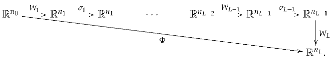
In their most basic form, $X_{\ell }$ is a finite set of $n_{\ell }$ elements and $V_{\ell }=\mathbb{R},$ a feed-forward neural network $\mathsf{\Phi }:{\mathbb{R}}^{n_0}\mapsto {\mathbb{R}}^{n_L}$ is a function of the following form: the input is $x^{(0)}=x\in {\mathbb{R}}^{n_0},$ $x^{(\ell )}={\sigma }_{\ell }(W_{\ell }(x^{(\ell -1)}))$ for $\ell =1,\dots ,L-1,$ and

$$\mathsf{\Phi }(x)=x^{(L)}=W_L({\sigma }_{L-1}(W_{L-1}\cdots {\sigma }_1(W_1(x^{(0)}))\cdots )),$$

(3)

where $x^{(L)}\in {\mathbb{R}}^{n_L}$ is the output. This can be illustrated as follows:

Here, the map $W_{\ell }:{\mathbb{R}}^{n_{\ell -1}}\mapsto {\mathbb{R}}^{n_{\ell }}$ is usually of the form

$$W_{\ell }{x}^{(\ell -1)}=A_{\ell }{x}^{(\ell -1)}+b_{\ell },\ell =1,\dots ,L,$$

(4)

where $A_{\ell }$ is an $n_{\ell }\times n_{\ell -1}$ matrix called a weight matrix and $b_{\ell }\in {\mathbb{R}}^{n_{\ell }}$ is called a bias vector for each $\ell ,$ and the function ${\sigma }_{\ell }:{\mathbb{R}}^{n_{\ell }}\mapsto {\mathbb{R}}^{n_{\ell }}$ represents the activation function at the ℓ-th layer. The set of all entries of the weight matrices and bias vectors of a neural network $\mathsf{\Phi }$ are called the parameters of $\mathsf{\Phi }.$ These parameters are adjustable and learned during the training process, determining the specific function realized by the network. Also, the depth $L,$ the number of neurons in each layer, and the activation functions of a neural network $\mathsf{\Phi }$ are called the hyperparameters of $\mathsf{\Phi }.$ They define the network’s architecture (and training process) and are typically set before training begins. For a fixed architecture, every choice of network parameters as in (3) defines a specific function $\mathsf{\Phi },$ and this function is often referred to as a model.

In a feed-forward neural network, the inputs to neurons in the ℓ-th layer are usually exclusively neurons from the $(\ell -1)$-th layer. However, residual neural networks (ResNets for short) allow skip connections; that is, information is allowed to skip layers in the sense that the neurons in layer ℓ may have $x^{(0)},\dots ,x^{(\ell -1)}$ as their input (and not just $x^{(\ell -1)}$). In their most basic form, $x^{(0)}=x\in {\mathbb{R}}^d,$ and

$$x^{(\ell )}=x^{(\ell -1)}+Q_{\ell }\sigma (A_{\ell }{x}^{(\ell -1)}+b_{\ell }),\ell =1,\dots ,L-1,$$

(5)

where $\sigma :{\mathbb{R}}^d\mapsto {\mathbb{R}}^d$ is a vector function, $Q_{\ell },A_{\ell }$’s are $d\times d$ matrices, and $b_{\ell }$’s are vectors in ${\mathbb{R}}^d.$ In contrast to feed-forward neural networks, recurrent neural networks (RNNs for short) allow information to flow backward in the sense that $x^{(\ell -1)},x^{(\ell +1)},\dots ,x^{(L)}$ may serve as input for the neurons in layer ℓ and not just $x^{(\ell -1)}.$ We refer to [12] for more details, such as training for a neural network.

2.2. Attention

The fundamental definition of attention was given by Bahdanau et al. in 2014. To describe the mathematical definition of attention, we denote by $\mathbb{Q}\subset {\mathbb{R}}^{d_q}$ the query space, $\mathbb{K}\subset {\mathbb{R}}^{d_k}$ the key space, and $\mathbb{V}\subset {\mathbb{R}}^{d_v}$ the value space. We call an element $q\in \mathbb{Q}$ a query, $k\in \mathbb{K}$ a key, $v\in \mathbb{V}$, and so on.

Definition 1 

(cf. [13]). Let $a:\mathbb{Q}\times \mathbb{K}\mapsto \mathbb{R}$ be a function. Let $K=\{k_1,\dots ,k_N\}\subset \mathbb{K}$ be a set of keys and $V\subset \mathbb{V}$ a set of values. Given a $q\in \mathbb{Q},$ the attention $\mathrm{Att}:(q,K,V)\mapsto \mathbb{R}$ is defined by

$$\mathrm{Att}(q,K,V)=\sum _{n=1}^N{\mathrm{softmatch}}_a{(q,K)}_n·v_n,$$

(6)

where ${\mathrm{softmatch}}_a(q,K)$ is a probability distribution over $K=\{k_1,\dots ,k_N\}$ defined by

$${\mathrm{softmatch}}_a{(q,K)}_n={\displaystyle \frac{e^{a(q,k_n)}}{{\sum }_{j=1}^N{e}^{a(q,k_j)}}},n=1,\dots ,N.$$

(7)

This means that a value $v_n$ in (6) occurs with probability ${\mathrm{softmatch}}_a{(q,K)}_n$ for $n\in \left[N\right].$

For $Q=\{q_1,\dots ,q_M\}\subset \mathbb{Q},$ we define

$$\mathrm{Att}(Q,K,V)={\left\{\mathrm{Att}(q_m,K,V)\right\}}_{m=1}^M.$$

(8)

In particular, when $Q=K=V,$ $\mathrm{Att}(Q,Q,Q)$ is said to be self-attention at $Q,$ and the mapping $\mathrm{SelfAtt}$ defined by

$$\mathrm{SelfAtt}(Q)=\mathrm{Att}(Q,Q,Q),$$

(9)

is called the self-attention map.

We remark that

(1)

For a finite sequence ${\left\{x_n\right\}}_{n=1}^N$ of real numbers, define

$$\mathrm{softmax}{(\{x_j)\}}_{j=1}^N{)}_n={\displaystyle \frac{e^{x_n}}{{\sum }_{j=1}^N{e}^{x_j}}},n\in \left[N\right].$$

(10)

Then,

$${\mathrm{softmatch}}_a{(q,K)}_n=\mathrm{softmax}{({\left\{a(q,k_j)\right\}}_{j=1}^N)}_n,$$

(11)

as usual in the literature.

(2)

We have $|K|=|V|=N,$ but $|Q|=M\ne N$ in general.

(3)

The function $a:\mathbb{Q}\times \mathbb{K}\mapsto \mathbb{R}$ is called a similarity function, usually given by

$$a(q,k)={\displaystyle \frac{1}{\sqrt{d^{\prime }}}}⟨W^{Q}q,W^{K}k⟩,$$

(12)

where $W^Q$ is a $d^{\prime }\times d_q$ real matrix called a query matrix and $W^K$ is a $d^{\prime }\times d_k$ real matrix called a key matrix. For $q\in \mathbb{Q},k\in \mathbb{K},$ the real number $a(q,k)$ is interpreted as the similarity between the query q and the key $k.$

(4)

In the representation learning framework of attention, we usually assume the finite set $\mathbf{T}$ of tokens has been embedded in ${\mathbb{R}}^d,$ where d is called the embedding dimension, so we identify each $t\in \mathbf{T}$ with one of finitely-many vectors x in ${\mathbb{R}}^d.$ We assume that the structure (positional information, adjacency information, etc) is encoded in these vectors. In the case of self-attention, we assume $d_q=d_k=d_v=d.$

Since the self-attention mechanism can be composed to arbitrary depth, making it a crucial building block of the transformer architecture, we mainly focus on it in what follows. In practice, we need multi-headed attention (cf. [4]), that process independent copies of the data X and combine them with concatenation and matrix multiplication. Let $X={\left\{x_n\right\}}_{n=1}^N$ be the input set of tokens embedded in ${\mathbb{R}}^d.$ Let us consider $n_h$-headed attention with the dimension $d_h$ for every head. For every $i\in \left[n_h\right],$ let $W_i^Q,W_i^K,W_i^V$ be $d_h\times d$ (query, key, value) matrices associated with the i-th self-attention, and the similarity function

$$a_i(x,y)={\displaystyle \frac{1}{\sqrt{d_h}}}⟨W_i^{Q}x,W_i^{K}y⟩.$$

(13)

Let $W^O=[W_1^O,\dots ,W_{n_h}^O]$ denote the output projection matrix, where $W_i^O$ is a $d\times d_h$ matrix for every $i\in \left[n_h\right].$ For $n\in \left[N\right],$ the multi-headed self-attention (MHSelfAtt for short) is then defined by

$$\mathrm{MHSelfAtt}(x_n,X,X)=\sum _{i=1}^{n_h}\sum _{j_i=1}^n\mathrm{softmax}{({\{{\displaystyle \frac{1}{\sqrt{d_h}}}⟨W_i^Q{x}_n,W_i^K{x}_{\ell }⟩\}}_{\ell =1}^n)}_{j_i}\left[W_i^O(W_i^V{x}_{j_i})\right],$$

(14)

that is, an output

$$u_n=\sum _{i=1}^{n_h}{W}_i^O(W_i^V{x}_{j_i}),j_i\in \left[n\right],$$

(15)

occurs with the probability ${\prod }_{i=1}^{n_h}\mathrm{softmax}{({\{{\displaystyle \frac{1}{\sqrt{d_h}}}⟨W_i^Q{x}_n,W_i^K{x}_{\ell }⟩\}}_{\ell =1}^n)}_{j_i}.$ As such,

$$\mathrm{MHSelfAtt}(X)={\left\{\mathrm{MHSelfAtt}(x_n,X,X)\right\}}_{n=1}^N,$$

(16)

yields a basic building block of the transformer

$$\mathrm{Transf}(X)=\mathrm{FFN}\circ \mathrm{MHSelfAtt}(X),$$

(17)

as in the case of one-headed attention.

2.3. Transformer

In line with successful models, such as large language models, we focus on the decoder-only setting of the transformer, where the model iteratively predicts the next tokens based on a given sequence of tokens. This procedure is called autoregressive since the prediction of new tokens is only based on previous tokens. Such conditional sequence generation using autoregressive transformers is referred to as the transformer architecture.

Specifically, in the transformer architecture defined by a composition of blocks, each block consists of a self-attention layer $\mathrm{SelfAtt},$ a multi-layer perception $\mathrm{FFN},$ and a prediction head layer $\mathrm{PH}.$ First, the self-attention layer SelfAtt is the only layer that combines different tokens. Let us denote the input text to the layer by $X={\left\{x_n\right\}}_{n=1}^N$ embedded in ${\mathbb{R}}^d$ and focus on the n-th output. For each $n\in \left[N\right],$ letting

$$s_j^{(n)}={\displaystyle \frac{1}{\sqrt{d}}}⟨W^Q{x}_n,W^K{x}_j⟩,\forall j\in \left[n\right],$$

(18)

where $W^Q$ and $W^K$ are two $d^{\prime }\times d$ matrices (i.e., the query and key matrices), we can interpret $S^{(n)}={\left\{s_j^{(n)}\right\}}_{j=1}^n$ as similarities between the n-th token $x_n$ (i.e., the query) and the other tokens (i.e., keys); for satisfying the autoregressive structure, we only consider $j=1,\dots ,n.$ The softmax layer is given by

$$\mathrm{softmax}{(S^{(n)})}_j={\displaystyle \frac{e^{s_j^{(n)}}}{{\sum }_{i=1}^n{e}^{s_i^{(n)}}}},\forall j\in \left[n\right],$$

(19)

which can be interpreted as the probability for the n-th query to “attend” to the j-th key. Then, the self-attention layer $\mathrm{SelfAtt}$ can be defined as

$$\mathrm{SelfAtt}{(X)}_n=\sum _{j=1}^n\mathrm{softmax}{(S^{(n)})}_j{W}^V{x}_j,n\in \left[N\right],$$

(20)

where $W^V$ is the $d\times d$ real matrix such that $W^{V}x\in \mathbf{T}$ for any $x\in \mathbf{T},$ the output $W^V{x}_j$ occurring with the probability $\mathrm{softmax}{(S^{(n)})}_j$ is often referred to as the values of the token $x_j.$ Thus, $\mathrm{SelfAtt}:{({\mathbb{R}}^d)}^{*}\mapsto {({\mathbb{R}}^d)}^{*}$ is a random map such that $\mathrm{SelfAtt}\left[{({\mathbb{R}}^d)}^{(N)}\right]\subset {({\mathbb{R}}^d)}^{(N)}$ for each $N\in \mathbb{N}.$

If the attention is a multi-headed attention with $n_h$ heads of the dimension $d_h,$ where for $i\in \left[n_h\right],$ $W_i^Q,W_i^K,W_i^V$ are the $d_h\times d$ (query, key, value) matrices and $W_i^O$ is the $d\times d_h$ (output) matrix of the i-th self-attention, then the multi-headed self-attention layer $\mathrm{MHSelfAtt}$ is defined by

$$\mathrm{MHSelfAtt}{(X)}_n=\sum _{i=1}^{n_h}\sum _{j_i=1}^n\mathrm{softmax}{(S_i^{(n)})}_{j_i}\left[W_i^O(W_i^V{x}_{j_i})\right],n\in \left[N\right],$$

(21)

where

$$\mathrm{softmax}{(S_i^{(n)})}_{j_i}={\displaystyle \frac{\frac{1}{\sqrt{d_h}}⟨W_i^Q{x}_n,W_i^K{x}_{j_i}⟩}{{\sum }_{\ell =1}^n\frac{1}{\sqrt{d_h}}⟨W_i^Q{x}_n,W_i^K{x}_{\ell }⟩}},j_i\in \left[n\right],$$

(22)

i.e., an output $u_n={\sum }_{i=1}^{n_h}{W}_i^O(W_i^V{x}_{j_i})$ occurs with the probability ${\prod }_{i=1}^{n_h}\mathrm{softmax}{(S_i^{(n)})}_{j_i}$ for each $n\in \left[N\right].$ In what follows, we only consider the case of one-headed attention, since the multi-headed case is similar.

Second, the multi-layer perception is a feed-forward neural network $\mathrm{FFN}$ such that $y_n=\mathrm{FFN}(W^V{x}_j)$ with the probability $\mathrm{softmax}{(S^{(n)})}_j$ ($j\in \left[n\right]$) for each $n\in \left[N\right].$ Finally, the prediction head layer can be represented as a mapping $\mathrm{PH}:{({\mathbb{R}}^d)}^{*}\mapsto {[0,1]}^{*},$ which maps the sequence of ${\left\{y_n\right\}}_{n=1}^N$ to a probability distribution ${\left\{p_n\right\}}_{n=1}^N,$ where $p_n$ is the probability of predicting $y_n$ as the next token. Since $y_N$ contains information about the whole input text, we may define

$$\mathrm{PH}\left[{\left\{y_n\right\}}_{n=1}^N\right]=\sum _{j=1}^N\mathrm{softmax}{(S^{(N)})}_j\mathrm{FFN}(W^V{x}_j),$$

(23)

such that the next token $x_{N+1}=y_j=\mathrm{FFN}(W^V{x}_j)$ with the probability $\mathrm{softmax}{(S^{(N)})}_j$ for $j\in \left[N\right].$

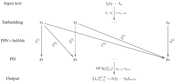
Hence, a basic building block for the transformer, consisting of a self-attention module (SelfAtt) and a feed-forward network (FFN) followed by a prediction head layer (PH), can be illustrated as follows:

where the input text $t_1{t}_2\dots t_n$ is embedded as a sequence ${\left\{x_i\right\}}_{i=1}^n$ in ${\mathbb{R}}^d,$ $y_j=\mathrm{FFN}(W^V{x}_j)$ occurs with the probability $\mathrm{softmax}{(S^{(n)})}_j$ for each $j\in \left[n\right],$ $x_{n+1}=y_j$ is generated with the probability $\mathrm{softmax}{(S^{(n)})}_j$ for each $j\in \left[n\right],$ and so the output is $x_{n+1}=\mathrm{PH}\circ \mathrm{FFN}\circ \mathrm{SelfAtt}({\left\{x_i\right\}}_{i=1}^n).$ One can then apply the same operations to the extended sequence $x_1{x}_2\dots x_n{x}_{n+1}$ in the next block, obtaining $x_{n+2}=\mathrm{PH}\circ \mathrm{FFN}\circ \mathrm{SelfAtt}({\left\{x_i\right\}}_{i=1}^{n+1}),$ to iteratively compute further tokens (there is usually a stopping criterion based on a special token or the mapping $\mathrm{PH}$). Below, without loss of generality, we omit the prediction head layer $\mathrm{PH}.$

Typically, a transformer of depth L is defined by a composition of L blocks, denoted by ${\mathrm{Transf}}_L,$ consisting of L self-attention maps ${\left\{{\mathrm{SelfAtt}}_{\ell }\right\}}_{\ell =1}^L$ and L feed-forward neural networks ${\left\{{\mathrm{FFN}}_{\ell }\right\}}_{\ell =1}^L,$ that is,

$${\mathrm{Transf}}_L=({\mathrm{FFN}}_L\circ {\mathrm{SelfAtt}}_L)\circ \cdots \circ ({\mathrm{FFN}}_1\circ {\mathrm{SelfAtt}}_1),$$

(24)

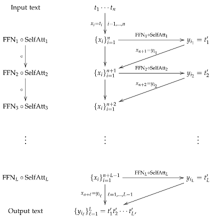
where the indices of the layers SelfAtt and FFN in (24) indicate the use of different trainable parameters in each of the blocks. This can be illustrated as follows:

that is,

$${\mathrm{Transf}}_L(t_1\cdots t_n)=t_1^{\prime }{t}_2^{\prime }\cdots t_L^{\prime }.$$

(25)

Also, we can consider the transformer of the form

$${\mathrm{Transf}}_L=((\mathrm{id}+{\mathrm{FFN}}_L)\circ (\mathrm{id}+{\mathrm{SelfAtt}}_L))\circ \cdots \circ ((\mathrm{id}+{\mathrm{FFN}}_1)\circ (\mathrm{id}+{\mathrm{SelfAtt}}_1)),$$

(26)

where $\mathrm{id}$ denotes the identity mapping in ${\mathbb{R}}^d,$ commonly known as a skip or residual connection.

2.4. Effect Algebras

For the sake of convenience, we collect some notations and basic properties of $\sigma$-effect algebras (cf. [1,11,14] and references therein). Recall that an effect algebra is an algebraic system $(\mathbf{E},0,1,\oplus ),$ where $\mathbf{E}$ is a non-empty set, $0,1\in \mathbf{E}$, which are called zeroes and unit elements of this algebra, respectively, and ⊕ is a partial binary operation on $\mathbf{E}$ that satisfies the following conditions for any $a,b,c\in \mathbf{E}$:

(E1)

(Commutative Law): If $a\oplus b$ is defined, then $b\oplus a$ is defined and $b\oplus a=a\oplus b,$ which is called the orthogonal sum of a and $b;$

(E2)

(Associative Law): If $a\oplus b$ and $(a\oplus b)\oplus c$ are defined, then $b\oplus c$ and $a\oplus (b\oplus c)$ are defined and

$$\begin{array}{c}\hfill (a\oplus b)\oplus c=a\oplus (b\oplus c),\end{array}$$

which is denoted by $a\oplus b\oplus c;$

(E3)

(Orthosupplementation Law): there exists a unique $a^{\prime }\in \mathbf{E}$ such that $a\oplus a^{\prime }$ is defined and $a\oplus a^{\prime }=1,$ such $a^{\prime }$ is unique and called the orthosupplement of $a;$

(E4)

(Zero–One Law): if $a\oplus 1$ is defined, then $a=0.$

We simply call $\mathbf{E}$ an effect algebra in the sequel. From the associative law (E2), we can write $a_1\oplus a_2\oplus \cdots \oplus a_n$ if this orthogonal sum is defined. For any $a,b\in \mathbf{E},$ we define $a\le b$ if there exists a $c\in \mathbf{E}$ such that $a\oplus c=b;$ this c is unique and denoted by $c=b\ominus a,$ so $a^{\prime }=1\ominus a.$ We also define $a\perp b$ if $a\oplus b$ is defined; i.e., a is orthogonal to $b.$ It can be shown (cf. [14]) that $(\mathbf{E},\le )$ is a bounded partially ordered set (poset for short) and $a\perp b$ if and only if $a\le b^{\prime }.$ For a sequence ${\left\{a_i\right\}}_{i=1}^{\infty }$ in $\mathbf{E},$ if $a_1\oplus \cdots \oplus a_n$ is defined for all $n\in \mathbb{N}$ such that ${\bigvee }_{n=1}^{\infty }(a_1\oplus \cdots \oplus a_n)$ exists, then the sum ${⨁}_i{a}_i$ of ${\left\{a_i\right\}}_{i=1}^{\infty }$ exists and define ${⨁}_i{a}_i={\bigvee }_{n=1}^{\infty }(a_1\oplus \cdots \oplus a_n).$ We say that $\mathbf{E}$ is a $\sigma$-effect algebra if ${⨁}_i{a}_i$ exists for any sequence ${\left\{a_i\right\}}_{i=1}^{\infty }$ in $\mathbf{E}$ satisfying that $a_1\oplus \cdots \oplus a_n$ is defined for all $n\in \mathbb{N}.$ It was shown in (Lemma 3.1, [1]) that $\mathbf{E}$ is a $\sigma$-effect algebra if and only if the least upper bound ${\bigvee }_i{a}_i$ exists for any monotone sequence ${\left\{a_i\right\}}_{i=1}^{\infty },$ i.e., $a_1\le a_2\le \cdots .$

Let $\mathbf{E}$ and $\mathbf{F}$ be $\sigma$-effect algebras. A map $\varphi :\mathbf{E}\mapsto \mathbf{F}$ is said to be additive if for $a,b\in \mathbf{E},$ $a\perp b$ implies that $\varphi (a)\perp \varphi (b)$ and $\varphi (a\oplus b)=\varphi (a)\oplus \varphi (b).$ An additive map $\varphi :\mathbf{E}\mapsto \mathbf{F}$ is $\sigma$-additive if for any sequence ${\left\{a_i\right\}}_{i=1}^{\infty }$ such that ${⨁}_i{a}_i$ exists, ${⨁}_i\varphi (a_i)$ exists and $\varphi ({⨁}_i{a}_i)={⨁}_i\varphi (a_i).$ A $\sigma$-additive map $\varphi :\mathbf{E}\mapsto \mathbf{F}$ is said to be a $\sigma$-morphism if $\varphi (1)=1;$ and moreover, $\varphi$ is called a $\sigma$-isomorphism if $\varphi$ is a bijective $\sigma$-morphism and ${\varphi }^{-1}:\mathbf{F}\mapsto \mathbf{E}$ is a $\sigma$-morphism. It can be shown (cf. [1]) that

(1)

A map $\varphi :\mathbf{E}\mapsto \mathbf{F}$ is additive if and only if $\varphi$ is monotone in the sense that $a\le b$ implies $\varphi (a)\le \varphi (b);$

(2)

An additive map $\varphi$ is $\sigma$-additive if and only if $a_1\le a_2\le \dots$ implies $\varphi ({\bigvee }_i{a}_i)={\bigvee }_i\varphi (a_i);$

(3)

A $\sigma$-morphism $\varphi$ satisfies $\varphi (a^{\prime })=\varphi {(a)}^{\prime }.$

The unit interval $[0,1]$ is a $\sigma$-effect algebra defined as follows: For any $a,b\in [0,1],$ $a\oplus b$ is defined if $a+b\le 1$ and in this case $a\oplus b=a+b.$ Then, we have that $a^{\prime }=1-a,$ and $0,1$ are the zero and unit elements, respectively. In what follows, we always regard $[0,1]$ as a $\sigma$-effect algebra in this way. Let $\mathbf{E}$ be a $\sigma$-effect algebra, a $\sigma$-morphism $\varphi :\mathbf{E}\mapsto [0,1]$ is called a state on $\mathbf{E},$ and we denote by $\mathcal{S}(\mathbf{E})$ the set of all states on $\mathbf{E}.$ A subset S of $\mathcal{S}(\mathbf{E})$ is said to be order determining if $\alpha (a)\le \alpha (b)$ for all $\alpha \in S$ implies $a\le b.$

Another example of a $\sigma$-effect algebra is a measurable space $(\mathsf{\Omega },\mathcal{F})$ defined as follows: For any $A,B\in \mathcal{F},$ $A\oplus B$ is defined if $A\cap B=\varnothing ,$ and in this case, $A\oplus B=A\cup B.$ We then have $0=\varnothing ,1=\mathsf{\Omega },$ and $A^{\prime }=\mathsf{\Omega }\setminus A.$ We always regard a measurable space $(\mathsf{\Omega },\mathcal{F})$ as a $\sigma$-effect algebra in this way. Let $\mathbf{E}$ be a $\sigma$-effect algebra, a $\sigma$-morphism $X:(\mathsf{\Omega },\mathcal{F})\mapsto \mathbf{E}$ is called an observable on $\mathbf{E}$ with values in $(\mathsf{\Omega },\mathcal{F})$ (a $\mathsf{\Omega }$-valued observable for short). The elements of a $\sigma$-effect algebra are called effects, and so an observable X maps effects in $\mathcal{F}$ into effects in $\mathbf{E}$; i.e., $X(A)$ is an effect in $\mathbf{E}$ for $A\in \mathcal{F}.$ We denote by $\mathcal{O}(\mathbf{E},\mathsf{\Omega },\mathcal{F})$ the set of all $\mathsf{\Omega }$-valued observables. Note that $\mathcal{S}(\mathsf{\Omega },\mathcal{F})$ is equal to the set of all probability measures on $(\mathsf{\Omega },\mathcal{F}).$ For $\alpha \in \mathcal{S}(\mathbf{E})$ and $X\in \mathcal{O}(\mathbf{E},\mathsf{\Omega },\mathcal{F}),$ we have $\alpha \circ X\in \mathcal{S}(\mathsf{\Omega },\mathcal{F}),$ which is called the probability distribution of X in the state $\alpha .$

3. Mathematical Formalism

In this section, we introduce a mathematical formalism for generative AI. We utilize the theory of $\sigma$-effect algebras to give a mathematical definition for a generative AI system. Let $\mathbf{E}$ be a $\sigma$-effect algebra and $(\mathsf{\Omega },\mathcal{F})$ a measurable space. An orthogonal decomposition in $\mathbf{E}$ is a sequence $\left\{a_i\right\}$ in $\mathbf{E}$ such that ${⨁}_i{a}_i$ exists, and moreover, it is complete if ${⨁}_i{a}_i=1.$ We denote by $\mathcal{D}(\mathbf{E})$ the set of all completely orthogonal decomposition in $\mathbf{E}.$ A completely orthogonal decomposition in $\mathcal{F}$ is called a countable partition of $\mathsf{\Omega },$ i.e., a sequence $\left\{A_i\right\}$ of elements in $\mathcal{F}$ such that $A_i\cap A_j$ for $i\ne j$ and ${\cup }_i{A}_i=\mathsf{\Omega }.$ We denote by $\mathcal{D}(\mathsf{\Omega },\mathcal{F})$ the set of all countable partitions of $\mathsf{\Omega }.$ For $n\in \mathbb{N},$ an ordered n-tuple $\overrightarrow{R}=(e_1,\dots ,e_n)$ of effects in $\mathbf{E}$ is called a n-time chain-of-effect, and we interpret $\overrightarrow{R}$ as an inference process of an intelligence machine in which the effect $e_i$ occurs at time ${\tau }_i$ for $i\in \left[n\right],$ where ${\tau }_1<{\tau }_2<\cdots <{\tau }_n.$ Alternatively, no specific times may be involved and we regard $\overrightarrow{R}$ as a sequential effect in which $e_1$ occurs first, $e_2$ occurs second, …, and $e_n$ occurs last.

Definition 2. 

With the above notations, a generative artificial intelligence system $\mathfrak{S}$ is defined to be a triple $(\mathbf{E},\mathsf{\Omega },\mathcal{F}),$ where $\mathbf{E}$ is a σ-effect algebra, $(\mathsf{\Omega },\mathcal{F})$ is a measurable space, such that

(G1) 

The input set $\mathbf{In}(\mathfrak{S})$ of $\mathfrak{S}$ is equal to the set $\mathcal{S}(\mathbf{E})$; i.e., an input is interpreted by a state $\alpha \in \mathcal{S}(\mathbf{E});$

(G2) 

The output set $\mathbf{Out}(\mathfrak{S})$ of $\mathfrak{S}$ is equal to the set ${\mathsf{\Omega }}^{*}={\bigcup }_{n=1}^{\infty }{\mathsf{\Omega }}^{(n)}$; i.e., the set of all finite sequences of elements in $\mathsf{\Omega };$

(G3) 

An inference process in $\mathfrak{S}$ is interpreted by a chain-of-effect $(e_1,\cdots ,e_n)$ for $n\in \mathbb{N}.$

Remark 1. 

We refer to [15] for a mathematical definition of general artificial intelligence systems in terms of topos theory, including quantum artificial intelligence systems.

In practice, we are not concerned with a generative AI system $\mathfrak{S}=(\mathbf{E},\mathsf{\Omega },\mathcal{F})$ itself but deal with models for $\mathfrak{S},$ such as large language models. To this end, we need to introduce the definition of a model for $\mathfrak{S}$ in terms of joint probability distributions for observables associated with $\mathfrak{S}.$

For $X\in \mathcal{O}(\mathbf{E},\mathsf{\Omega },\mathcal{F})$ and $A\in \mathcal{F},$ we may view the effect $X(A)$ as the event for which X has a value in $A.$ For a partition $\mathbf{D}=\left\{A_i\right\}\in \mathcal{D}(\mathsf{\Omega },\mathcal{F}),$ we may view $(X,\mathbf{D})$ as a set of possible alternative events that can occur. One interpretation is that $(X,\mathbf{D})$ represents a building block of an artificial intelligence architecture for processing X and the alternatives result from the dial readings of the block. Given $X_i\in \mathcal{O}(\mathbf{E},\mathsf{\Omega },\mathcal{F}),$ $A_i\in \mathcal{F},$ $i=1,\dots ,n,$ an ordered n-tuple $\overrightarrow{R}=(X_1(A_1),\dots ,X_n(A_n))$ of events is called an n-time chain-of-event, and we interpret $\overrightarrow{R}$ as an inference process of an intelligence machine in which $X_1$ has a value $a_1$ in $A_1$ first, $X_2$ has $a_2$ in $A_2$ s, …, and $X_n$ has $a_n$ in $A_n$ last, so that the output result is $(a_1,a_2,\dots ,a_n).$ We denote the set of all n-time chain-of-events by ${\mathbf{R}}^{(n)}$ and the set of all chain-of-events by ${\mathbf{R}}^{*}={\bigcup }_n{\mathbf{R}}^{(n)}.$

A n-step inference set has the form $\overrightarrow{\mathbf{I}}=((X_1,{\mathbf{D}}_1),\dots ,(X_n,{\mathbf{D}}_n)),$ where $X_i\in \mathcal{O}(\mathbf{E},\mathsf{\Omega },\mathcal{F}),$ ${\mathbf{D}}_i\in \mathcal{D}(\mathsf{\Omega },\mathcal{F}),$ $i\in \left[n\right].$ We interpret $\overrightarrow{\mathbf{I}}$ as ordered successive processes of observables $X_i$ with partitions ${\mathbf{D}}_i$ for $i\in \left[n\right].$ We denote the collection of all n-step inference sets by ${\mathbf{I}}^{(n)}$ and the collection of all inference sets by ${\mathbf{I}}^{*}={\bigcup }_n{\mathbf{I}}^{(n)}.$ If $\overrightarrow{R}=(X_1(A_1),\dots ,X_n(A_n))$ and $\overrightarrow{\mathbf{I}}=((X_1,{\mathbf{D}}_1),\dots ,(X_n,{\mathbf{D}}_n))$ such that $A_i\in {\mathbf{D}}_i$ for every $i\in \left[n\right],$ we say the chain-of-event $\overrightarrow{R}$ is an element of the inference set $\overrightarrow{\mathbf{I}}$ and write $\overrightarrow{R}\in \overrightarrow{\mathbf{I}}.$ 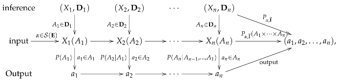This can be illustrated as follows:

which means that the machine firstly obtains $a_1$ as part of an output with the probability $P(A_1),$ then obtains $a_2$ with the conditional probability $P(A_2|A_1),$ …, and lastly obtains $a_n$ with the conditional probability $P(A_n|A_{n-1},\dots ,A_1)$ and finally combines them to obtain the output result $(a_1,a_2,\dots ,a_n)$ with the probability

$$P_{\alpha ,\overrightarrow{\mathbf{I}}}(A_1\times \cdots \times A_n)=P(A_1)P(A_2|A_1)\cdots P(A_n|A_{n-1},\dots ,A_1),$$

(27)

where $P_{\alpha ,\overrightarrow{\mathbf{I}}}$ will be explained later.

If ${\overrightarrow{\mathbf{I}}}_1=((X_1,{\mathbf{D}}_1),\dots ,(X_n,{\mathbf{D}}_n))$ and ${\overrightarrow{\mathbf{I}}}_2=((Y_1,{\mathbf{J}}_1),\dots ,(Y_m,{\mathbf{J}}_m))$ are two inference sets, then we define their sequential product by

$$\overrightarrow{\mathbf{I}}={\overrightarrow{\mathbf{I}}}_1{\overrightarrow{\mathbf{I}}}_2=((X_1,{\mathbf{D}}_1),\dots ,(X_n,{\mathbf{D}}_n),(Y_1,{\mathbf{J}}_1),\dots ,(Y_m,{\mathbf{J}}_m)),$$

(28)

and obtain a $(n+m)$-step inference set. Mathematically, we can include the empty inference set ∅ that satisfies $\varnothing \overrightarrow{\mathbf{I}}=\overrightarrow{\mathbf{I}}\varnothing =\overrightarrow{\mathbf{I}},$ such that ${\mathbf{I}}^{*}$ becomes a semigroup under this product.

For a partition $\mathbf{D}\in \mathcal{D}(\mathsf{\Omega },\mathcal{F}),$ we denote by $\sigma (\mathbf{D})$ the $\sigma$-subalgebra of $\mathcal{F}$ generated by $\mathbf{D},$ and for n partitions ${\left\{{\mathbf{D}}_i\right\}}_{i=1}^n,$ we denote by $\sigma ({\left\{{\mathbf{D}}_i\right\}}_{i=1}^n)$ the $\sigma$-algebra on ${\mathsf{\Omega }}^{(n)}$ generated by ${\left\{{\mathbf{D}}_i\right\}}_{i=1}^n,$ i.e.,

$$\sigma ({\left\{{\mathbf{D}}_i\right\}}_{i=1}^n)=\sigma (\{A_1\times \cdots \times A_n\subseteq {\mathsf{\Omega }}^{(n)}:A_i\in {\mathbf{D}}_i,i\in \left[n\right]\}).$$

(29)

We denote by $\mathcal{P}({\mathsf{\Omega }}^{(n)},\sigma ({\left\{{\mathbf{D}}_i\right\}}_{i=1}^n))$ the set of all probability measures on $({\mathsf{\Omega }}^{(n)},\sigma ({\left\{{\mathbf{D}}_i\right\}}_{i=1}^n)).$ Also, we write $\sigma (\overrightarrow{\mathbf{I}})=\sigma ({\left\{{\mathbf{D}}_i\right\}}_{i=1}^n)$ for $\overrightarrow{\mathbf{I}}=((X_1,{\mathbf{D}}_1),\dots ,(X_n,{\mathbf{D}}_n)).$ Given an input $\alpha \in \mathcal{S}(\mathbf{E}),$ for an inference set $\overrightarrow{\mathbf{I}}=((X_1,{\mathbf{D}}_1),\dots ,(X_n,{\mathbf{D}}_n))$, we denote by $P_{\alpha ,\overrightarrow{\mathbf{I}}}\in \mathcal{P}({\mathsf{\Omega }}^{(n)},\sigma (\overrightarrow{\mathbf{I}}))$ the probability measure such that for $A_1\times \cdots \times A_n\in \sigma ({\left\{{\mathbf{D}}_i\right\}}_{i=1}^n),$ $P_{\alpha ,\overrightarrow{\mathbf{I}}}(A_1\times \cdots \times A_n)$ is the probability within the inference set $\overrightarrow{\mathbf{I}}$ that the event $X_1(A_1)$ occurs first, $X_2(A_2)$ occurs second, …, $X_n(A_n)$ occurs last. We call $P_{\alpha ,\overrightarrow{\mathbf{I}}}\in \mathcal{P}({\mathsf{\Omega }}^{(n)},\sigma (\overrightarrow{\mathbf{I}}))$ the joint probability distribution of an inference set $\overrightarrow{\mathbf{I}}$ under the input $\alpha \in \mathcal{S}(\mathbf{E}).$

For interpreting a model for a generative AI system, $P_{\alpha ,\overrightarrow{\mathbf{I}}}$’s need to satisfy physically motivated axioms as follows.

Definition 3. 

With the above notations, a model $\mathcal{M}$ for $\mathfrak{S}=(\mathbf{E},\mathsf{\Omega },\mathcal{F})$ is defined to be a family of joint probability distributions of inference sets

$$\mathcal{M}=\bigcup _{n\in \mathbb{N}}\left\{P_{\alpha ,\overrightarrow{\mathbf{I}}}\in \mathcal{P}({\mathsf{\Omega }}^{(n)},\sigma (\overrightarrow{\mathbf{I}})):\alpha \in \mathcal{S}(\mathbf{E}),\overrightarrow{\mathbf{I}}\in {\mathbf{I}}^{(n)}\right\},$$

(30)

that satisfies the following axioms:

(P1) 

For ${\overrightarrow{\mathbf{I}}}_1=(X,\mathbf{D}),{\overrightarrow{\mathbf{I}}}_2=(Y,\mathbf{J})\in {\mathbf{I}}^{(1)}$ and $A\in \sigma (\mathbf{D}),B\in \sigma (\mathbf{J}),$ if $P_{\alpha ,{\overrightarrow{\mathbf{I}}}_1}(A)=P_{\alpha ,{\overrightarrow{\mathbf{I}}}_2}(B)$ for all $\alpha \in \mathcal{S}(\mathbf{E}),$ then $X(A)=Y(B).$

(P2) 

For $\overrightarrow{\mathbf{I}}\in {\mathbf{I}}^{*},$ ${\overrightarrow{\mathbf{I}}}_i=(X,{\mathbf{D}}_i),i=1,2,$ if $A\in \sigma (\overrightarrow{\mathbf{I}})$ and $B\in \sigma ({\mathbf{D}}_1)\cap \sigma ({\mathbf{D}}_2),$ then

$$P_{\alpha ,\overrightarrow{\mathbf{I}}{\overrightarrow{\mathbf{I}}}_1}(A\times B)=P_{\alpha ,\overrightarrow{\mathbf{I}}{\overrightarrow{\mathbf{I}}}_2}(A\times B),$$

(31)

for every $\alpha \in \mathcal{S}(\mathbf{E}).$

(P3) 

For $\overrightarrow{\mathbf{I}}\in {\mathbf{I}}^{*},$ $\overrightarrow{\mathbf{J}}=(X,\mathbf{D})$ with $\mathbf{D}=\left\{B_i\right\},$ if $A\in \sigma (\overrightarrow{\mathbf{I}})$ then

$$P_{\alpha ,\overrightarrow{\mathbf{I}}\overrightarrow{\mathbf{J}}}(A\times \mathsf{\Omega })=\sum _i{P}_{\alpha ,\overrightarrow{\mathbf{I}}\overrightarrow{\mathbf{J}}}(A\times B_i)=P_{\alpha ,\overrightarrow{\mathbf{I}}}(A),\forall \alpha \in \mathcal{S}(\mathbf{E}).$$

(32)

(P4) 

If ${\overrightarrow{\mathbf{I}}}_1=((X_1,{\mathbf{D}}_1),\dots ,(X_n,{\mathbf{D}}_n)),$ ${\overrightarrow{\mathbf{I}}}_2=((X_1,{\mathbf{J}}_1),\dots ,(X_n,{\mathbf{J}}_n)),$ and $A_i\in {\mathbf{D}}_i\cap {\mathbf{J}}_i$ for $i\in \left[n\right],$ then

$$P_{\alpha ,{\overrightarrow{\mathbf{I}}}_1}(A_1\times \cdots \times A_n)=P_{\alpha ,{\overrightarrow{\mathbf{I}}}_2}(A_1\times \cdots \times A_n),$$

(33)

for every $\alpha \in \mathcal{S}(\mathbf{E}).$

For the physical meanings of the model structure axioms, we remark that

(1)

The axiom $(\mathrm{P}1)$ means that the input set can distinguish different events;

(2)

The axiom $(\mathrm{P}2)$ means that the partition of the last processing is irrelevant;

(3)

The axiom $(\mathrm{P}3)$ means that the last processing does not affect the previous ones;

(4)

The axiom $(\mathrm{P}4)$ means that the probability of a chain of events does not depend on the partitions and hence is unambiguous. However, for $B\in \sigma ({\overrightarrow{\mathbf{I}}}_1)\cap \sigma ({\overrightarrow{\mathbf{I}}}_2)$ in $(\mathrm{P}4),$ $P_{\alpha ,{\overrightarrow{\mathbf{I}}}_1}(B)\ne P_{\alpha ,{\overrightarrow{\mathbf{I}}}_2}(B)$ in general if $X_i$’s are quantum observables due to quantum interference.

If ${\overrightarrow{\mathbf{I}}}_1=((X_1,{\mathbf{D}}_1),\dots ,(X_n,{\mathbf{D}}_n))$ and ${\overrightarrow{\mathbf{I}}}_2=((Y_1,{\mathbf{J}}_1),\dots ,(Y_m,{\mathbf{J}}_m))$ are two inference sets, $A\in \sigma ({\left\{{\mathbf{D}}_i\right\}}_{i=1}^n),$ $B\in \sigma ({\left\{{\mathbf{J}}_j\right\}}_{j=1}^m),$ and if $\alpha$ is an input such that $P_{\alpha ,{\overrightarrow{\mathbf{I}}}_1}(A)\ne 0,$ then we define the conditional probability of B given A within ${\overrightarrow{\mathbf{I}}}_1{\overrightarrow{\mathbf{I}}}_2$ under the input $\alpha$ as follows:

$$P_{\alpha ,{\overrightarrow{\mathbf{I}}}_2|{\overrightarrow{\mathbf{I}}}_1}(B|A)={\displaystyle \frac{P_{\alpha ,{\overrightarrow{\mathbf{I}}}_1{\overrightarrow{\mathbf{I}}}_2}(A\times B)}{P_{\alpha ,{\overrightarrow{\mathbf{I}}}_1}(A)}}.$$

(34)

Since $P_{\alpha ,{\overrightarrow{\mathbf{I}}}_1{\overrightarrow{\mathbf{I}}}_2}$ is a probability measure on $({\mathsf{\Omega }}^{(n+m)},\sigma ({\left\{{\mathbf{D}}^{\prime }\right\}}_{i=1}^{n+m})),$ where ${\mathbf{D}}_i^{\prime }={\mathbf{D}}_i$ for $i\in \left[n\right]$ and ${\mathbf{D}}_{n+j}^{\prime }={\mathbf{J}}_j$ for $j\in \left[m\right],$ so $P_{\alpha ,{\overrightarrow{\mathbf{I}}}_2|{\overrightarrow{\mathbf{I}}}_1}(-|A)$ is a probability measure on $({\mathsf{\Omega }}^m,\sigma ({\left\{\mathbf{J}\right\}}_{j=1}^m)),$ which is called a conditional sequential joint probability distribution.

Proposition 1. 

Given $\alpha \in \mathcal{S}(\mathbf{E}),$ $\overrightarrow{\mathbf{I}}\in {\mathbf{I}}^{*}$ and $A\in \sigma (\overrightarrow{\mathbf{I}}),$ if $P_{\alpha ,\overrightarrow{\mathbf{I}}}(A)\ne 0,$ then the conditional sequential joint probability distribution $P_{\alpha ,-|\overrightarrow{\mathbf{I}}}(-|A)$ satisfies the axioms (P2)–(P4) in Definition 3.

Proof. 

By the axiom (P2), we have

$$\begin{array}{c}\hfill P_{\alpha ,{\overrightarrow{\mathbf{I}}}_1{\overrightarrow{\mathbf{I}}}_2|\overrightarrow{\mathbf{I}}}(B\times C|A)={\displaystyle \frac{P_{\alpha ,\overrightarrow{\mathbf{I}}{\overrightarrow{\mathbf{I}}}_1{\overrightarrow{\mathbf{I}}}_2}(A\times B\times C)}{P_{\alpha ,\overrightarrow{\mathbf{I}}}(A)}}={\displaystyle \frac{P_{\alpha ,\overrightarrow{\mathbf{I}}{\overrightarrow{\mathbf{I}}}_1{\overrightarrow{\mathbf{I}}}_2^{\prime }}(A\times B\times C)}{P_{\alpha ,\overrightarrow{\mathbf{I}}}(A)}}=P_{\alpha ,{\overrightarrow{\mathbf{I}}}_1{\overrightarrow{\mathbf{I}}}_2^{\prime }|\overrightarrow{\mathbf{I}}}(B\times C|A);\end{array}$$

hence, $P_{\alpha ,-|\overrightarrow{\mathbf{I}}}(-|A)$ satisfies the axiom (P2), and so does the axiom (P3). Similarly, the axiom (P4) implies that $P_{\alpha ,-|\overrightarrow{\mathbf{I}}}(-|A)$ satisfies the axiom (P4); we omit the details. □

We remark that when observables are quantum ones, Bayes’ formula need not hold, i.e.,

$$P_{\alpha ,{\overrightarrow{\mathbf{I}}}_2|{\overrightarrow{\mathbf{I}}}_1}(B|A)P_{\alpha ,{\overrightarrow{\mathbf{I}}}_1}(A)\ne P_{\alpha ,{\overrightarrow{\mathbf{I}}}_1|{\overrightarrow{\mathbf{I}}}_2}(A|B)P_{\alpha ,{\overrightarrow{\mathbf{I}}}_2}(B),$$

(35)

in general. This is because the left-hand side is $P_{\alpha ,{\overrightarrow{\mathbf{I}}}_1{\overrightarrow{\mathbf{I}}}_2}(A\times B)$ and the right-hand side is $P_{\alpha ,{\overrightarrow{\mathbf{I}}}_2{\overrightarrow{\mathbf{I}}}_1}(B\times A),$ so the order of the occurrences is changed. For instance, consider a qubit with the standard basis $|0⟩$ and $|1⟩.$ Let $|x⟩={\displaystyle \frac{1}{\sqrt{2}}}(|0⟩+|1⟩).$ If $X_1(A)=|0⟩⟨0|,$ $X_2(B)=|x⟩⟨x|,$ and $\alpha =|0⟩⟨0|$; then

$$\begin{array}{c}\hfill P_{\alpha ,{\overrightarrow{\mathbf{I}}}_1{\overrightarrow{\mathbf{I}}}_2}(A\times B)=\mathrm{Tr}[\alpha {(X_2{\left(B\right)}^{{\displaystyle \frac{1}{2}}}{X}_1{\left(A\right)}^{{\displaystyle \frac{1}{2}}})}^{†}{X}_2{\left(B\right)}^{{\displaystyle \frac{1}{2}}}{X}_1{\left(A\right)}^{{\displaystyle \frac{1}{2}}}]=\mathrm{Tr}[\alpha X_1{\left(A\right)}^{{\displaystyle \frac{1}{2}}}{X}_2\left(B\right)X_1{\left(A\right)}^{{\displaystyle \frac{1}{2}}}]={\displaystyle \frac{1}{2}},\\ \hfill P_{\alpha ,{\overrightarrow{\mathbf{I}}}_2{\overrightarrow{\mathbf{I}}}_1}(B\times A)=\mathrm{Tr}[\alpha {(X_1{\left(A\right)}^{{\displaystyle \frac{1}{2}}}{X}_2{\left(B\right)}^{{\displaystyle \frac{1}{2}}})}^{†}{X}_1{\left(A\right)}^{{\displaystyle \frac{1}{2}}}{X}_2{\left(B\right)}^{{\displaystyle \frac{1}{2}}}]=\mathrm{Tr}[\alpha X_2{\left(B\right)}^{{\displaystyle \frac{1}{2}}}{X}_1\left(A\right)X_2{\left(B\right)}^{{\displaystyle \frac{1}{2}}}]={\displaystyle \frac{1}{4}},\end{array}$$

and so, $P_{\alpha ,{\overrightarrow{\mathbf{I}}}_2|{\overrightarrow{\mathbf{I}}}_1}(B|A)P_{\alpha ,{\overrightarrow{\mathbf{I}}}_1}(A)\ne P_{\alpha ,{\overrightarrow{\mathbf{I}}}_1|{\overrightarrow{\mathbf{I}}}_2}(A|B)P_{\alpha ,{\overrightarrow{\mathbf{I}}}_2}(B).$ We refer to Section 4 for more details.

4. Physical Models for Generative AI

Physical models for generative AI are usually described by using systems of mean-field interacting particles, such as large language models based on attention mechanisms (cf. [7,8] and references therein); i.e., generative AI systems are regarded as classical statistical ensembles. However, since modern chips process data through controlling the flow of electric current, i.e., the dynamics of largely many electrons, they should be regarded as quantum statistical ensembles from a physical perspective (cf. [10]). Consequently, we need to model modern intelligence machines involving open quantum systems. To this end, combining the history theory of quantum systems (cf. [2]) and the theory of effect algebras (cf. [1,14]), we construct physical models realizing generative AI systems as open quantum systems.

Let $\mathbb{H}$ be a separable complex Hilbert space with the inner product $⟨-|-⟩$ being conjugate-linear at the first variable and linear at the second variable. We denote by $\mathcal{L}(\mathbb{H})$ the set of all bounded linear operators on $\mathbb{H},$ by $\mathcal{O}(\mathbb{H})$ the set of all bounded self-adjoint operators, and by $\mathcal{P}(\mathbb{H})$ the set of all orthogonal projection operators. We denote by I the identity operator on $\mathbb{H}.$ Unless stated otherwise, an operator means a bounded linear operator in the sequel. An operator T is positive if $⟨x|Tx⟩\ge 0$ for all $x\in \mathbb{H},$ and in this case we write $T\ge 0.$ We define $\mathrm{Tr}\left[T\right]={\sum }_i⟨x_i|T{x}_i⟩$ for a positive operator $T,$ where $\left\{x_i\right\}$ is an orthogonal basis of $\mathbb{H}.$ It is known that $\mathrm{Tr}\left[T\right]$ is independent of the choice of the basis, and it is called the trace of T if $\mathrm{Tr}\left[T\right]<\infty .$ A positive operator $\rho$ is a density operator if $\mathrm{Tr}\left[\rho \right]=1,$ and the set of all density operators on $\mathbb{H}$ is denoted by $\mathcal{S}(\mathbb{H}).$ Each positive operator is self-adjoint, and if two self-adjoint operators $S,T$ such that $T-S\ge 0,$ we write $T\ge S$ or $S\le T.$ We refer to [16,17,18] for more details on the theory of operators on Hilbert spaces.

A self-adjoint operator E that satisfies $0\le E\le I$ is called an effect, and the set of all effects on $\mathbb{H}$ is denoted by $\mathcal{E}(\mathbb{H}).$ For $E,F\in \mathcal{E}(\mathbb{H}),$ we define $E\oplus F=E+F$ if $E+F\le I,$ and in this case we write $E\perp F.$ It can be shown (cf. (Lemma 5.1, [1])) that $(\mathcal{E}(\mathbb{H}),0,I,\oplus )$ is a $\sigma$-effect algebra, and each state $\alpha$ on $\mathcal{E}(\mathbb{H})$ has the form $\alpha (E)=\mathrm{Tr}\left[\rho E\right]$ for every $E\in \mathcal{E}(\mathbb{H}),$ where $\rho$ is a unique density operator on $\mathbb{H},$ and vice versa. Thus, we identify $\mathcal{S}(\mathcal{E}(\mathbb{H}))=\mathcal{S}(\mathbb{H}).$ Let $(\mathsf{\Omega },\mathcal{F})$ be a measurable space. An observable $X\in \mathcal{O}(\mathcal{E}(\mathbb{H}),\mathsf{\Omega },\mathcal{F})$ is a positive operator valued (POV for short) measure on $(\mathsf{\Omega },\mathcal{F})$; i.e.,

(1)

$X(F)$ is an effect on $\mathcal{E}(\mathbb{H})$ for any $F\in \mathcal{F};$

(2)

$X(\varnothing )=0$ and $X(\mathsf{\Omega })=I;$

(3)

For an orthogonal decomposition $\left\{F_j\right\}$ in $\mathcal{F},$

$$X(\bigcup _j{F}_j)=\sum _{j}X(F_j),$$

(36)

where the series on the right-hand side is convergent in the strong operator topology on $\mathcal{L}(\mathbb{H}),$ i.e.,

$$X(\bigcup _j{F}_j)h=\sum _{j}X(F_j)h,$$

(37)

for every $h\in \mathbb{H}.$

To understand the inference process, let us show the conventional interpretation of joint probability distributions in an open quantum system that is subject to measurements by an external observer. To this end, let $\mathcal{E}(t,s)=\left\{K_m(t,s)\right\}$ denote the time-evolution operator from time s to $t,$ where $K_m(t,s)$’s are usually called Kraus operators, such that

$$\sum _m{K}_m{(t,s)}^{†}{K}_m(t,s)=I.$$

(38)

That is, $\mathcal{E}(t,s)$ are quantum operations (cf. [19]) such that for every state $\rho \in \mathcal{S}(\mathbb{H}),$

$$\mathcal{E}(t,s)\rho =\sum _m{K}_m(t,s)\rho K_m{(t,s)}^{†},$$

(39)

in the Schrödinger picture, while for each observable $X\in \mathcal{O}(\mathbb{H}),$

$$\mathcal{E}(t,s)X=\sum _m{K}_m{(t,s)}^{†}X{K}_m(t,s),$$

(40)

in the Heisenberg picture. We refer to [9] for the details on the theory of open quantum systems.

Then the density operator state $\rho (t_0)$ at time $t_0$ evolves in time $t_1-t_0$ to the state $\rho (t_1),$ where

$$\rho (t_1)=\mathcal{E}(t_1,t_0)\rho (t_0)=\sum _m{K}_m(t_1,t_0)\rho (t_0)K_m{(t_1,t_0)}^{†}.$$

(41)

Suppose that a measurement $(X_1,{\mathbf{D}}_1)$ is made at time $t_1,$ where $X_1\in \mathcal{O}(\mathcal{E}(\mathbb{H}),\mathsf{\Omega },\mathcal{F})$ and ${\mathbf{D}}_1\in \mathcal{D}(\mathsf{\Omega },\mathcal{F}).$ Then the probability that an event $X_1(A_1)$ with $A_1\in {\mathbf{D}}_1$ occurs is

$$\mathrm{P}(X_1(A_1),\rho (t_1))=\mathrm{Tr}\left[X_1(A_1)\rho (t_1)\right].$$

(42)

If the result of this measurement is kept, then, according to the von Neumann–Lüders reduction postulate, the appropriate density operator to use for any further calculation is

$${\rho }_{\mathrm{red}}(t_1)={\displaystyle \frac{X_1{(A_1)}^{\frac{1}{2}}\rho (t_1)X_1{(A_1)}^{\frac{1}{2}}}{\mathrm{Tr}\left[X_1(A_1)\rho (t_1)\right]}}.$$

(43)

Next, suppose a measurement $(X_2,{\mathbf{D}}_2)$ is performed at time $t_2>t_1.$ Then, according to the above, the conditional probability of an event $X_2(A_2)$ for $A_2\in {\mathbf{D}}_2$ occurs at time $t_2$ given that the event $X_1(A_1)$ occurs at time $t_1$ (and that the original state was $\rho (t_0)$) is

$$\mathrm{P}(X_2(A_2)|X_1(A_1),\rho (t_0))=\mathrm{Tr}\left[X_2(A_2)\rho (t_2)\right],$$

(44)

where $\rho (t_2)=\mathcal{E}(t_2,t_0){\rho }_{\mathrm{red}}(t_1),$ and the appropriate density operator to use for any further calculation is

$${\rho }_{\mathrm{red}}(t_2)={\displaystyle \frac{X_2{(A_2)}^{\frac{1}{2}}\rho (t_2)X_2{(A_2)}^{\frac{1}{2}}}{\mathrm{Tr}\left[X_2(A_2)\rho (t_2)\right]}}.$$

(45)

The joint probability of $X_1(A_1)$ occurring at $t_1$ and $X_2(A_2)$ occurring at $t_2$ is then

$$\begin{array}{cc}\hfill \mathrm{P}((X_1(A_1),X_2(A_2)),\rho (t_0))=& \mathrm{P}(X_1(A_1),\rho (t_1))\mathrm{P}(X_2(A_2)|X_1(A_1),\rho (t_0))\hfill \\ \hfill =& \mathrm{Tr}\left[X_1(A_1)\rho (t_1)\right]\mathrm{Tr}\left[X_2(A_2)\rho (t_2)\right].\hfill \end{array}$$

(46)

Generalizing to a sequence of measurements $(X_1,{\mathbf{D}}_1),(X_2,{\mathbf{D}}_2),\dots ,(X_n,{\mathbf{D}}_2)$ at times $t_1<t_2<\cdots <t_n,$ where $X_i\in \mathcal{O}(\mathcal{E}(\mathbb{H}),\mathsf{\Omega },\mathcal{F})$ and ${\mathbf{D}}_i\in \mathcal{D}(\mathsf{\Omega },\mathcal{F})$ for $i\in \left[n\right],$ the sequential joint probability of associated events $X_i(A_i)$ with $A_i\in {\mathbf{D}}_i$ occurring at $t_i$ for $i\in \left[n\right]$ is

$$\begin{array}{cc}\hfill \mathrm{P}((X_1& (A_1),X_2(A_2),\dots ,X_n(A_n)),\rho (t_0))\hfill \\ \hfill =& \mathrm{Tr}\left[X_1(A_1)\rho (t_1)\right]\mathrm{Tr}\left[X_2(A_2)\rho (t_2)\right]\cdots \mathrm{Tr}\left[X_n(A_n)\rho (t_n)\right],\hfill \end{array}$$

(47)

where $\rho (t_i)=\mathcal{E}(t_i,t_0){\rho }_{\mathrm{red}}(t_{i-1})$ for $i\in \left[n\right],$ ${\rho }_{\mathrm{red}}(t_0)=\rho (t_0),$ and

$${\rho }_{\mathrm{red}}(t_i)={\displaystyle \frac{X_i{(A_i)}^{\frac{1}{2}}\rho (t_i)X_i{(A_i)}^{\frac{1}{2}}}{\mathrm{Tr}\left[X_i(A_i)\rho (t_i)\right]}}.$$

(48)

for $i\in [n-1].$

Therefore, given an inference set $\overrightarrow{\mathbf{I}}=((X_1,{\mathbf{D}}_1),\dots ,(X_n,{\mathbf{D}}_n)),$ for an input $\rho (t_0)\in \mathcal{S}(\mathbf{E}),$ the sequential joint probability within the inference set $\overrightarrow{\mathbf{I}}$ that the event $X_1(A_1)$ occurs at $t_1,$ $X_2(A_2)$ occurs at $t_2,$ …, $X_n(A_n)$ occurs at $t_n,$ where $A_i\in {\mathbf{D}}_i$ for $i\in \left[n\right]$ and $t_0<t_1<t_2<\cdots <t_n,$ is given by

$$\begin{array}{c}\hfill P_{\rho (t_0),\overrightarrow{\mathbf{I}}}(A_1\times \cdots \times A_n)=\mathrm{Tr}\left[X_1(A_1)\rho (t_1)\right]\mathrm{Tr}\left[X_2(A_2)\rho (t_2)\right]\cdots \mathrm{Tr}\left[X_n(A_n)\rho (t_n)\right],\end{array}$$

(49)

where $\rho (t_i)=\mathcal{E}(t_i,t_0){\rho }_{\mathrm{red}}(t_{i-1})$ and

$$\mathcal{E}(t_i,t_0){\rho }_{\mathrm{red}}(t_{i-1})=\sum _m{K}_m(t_i,t_0){\rho }_{\mathrm{red}}(t_{i-1})K_m{(t_i,t_0)}^{†},$$

(50)

for $i\in \left[n\right],$ in the Schrödinger picture operator defined with respect to the fiducial time $t_0.$

Proposition 2. 

Let $\mathbb{H}$ be a separable complex Hilbert space, and let $(\mathsf{\Omega },\mathcal{F})$ be a measurable space. A physical model associated with $(\mathcal{E}(\mathbb{H}),\mathsf{\Omega },\mathcal{F})$ defined by

$$\mathcal{M}=\bigcup _{n\in \mathbb{N}}\left\{P_{\rho ,\overrightarrow{\mathbf{I}}}\in \mathcal{P}({\mathsf{\Omega }}^{(n)},\sigma (\overrightarrow{\mathbf{I}})):\rho \in \mathcal{S}(\mathbb{H}),\overrightarrow{\mathbf{I}}\in {\mathbf{I}}^{(n)}\right\},$$

(51)

where $P_{\rho ,\overrightarrow{\mathbf{I}}}$s’ are given by (49), satisfies the axioms in Definition 3.

Proof. 

For ${\overrightarrow{\mathbf{I}}}_1=(X,\mathbf{D}),{\overrightarrow{\mathbf{I}}}_2=(Y,\mathbf{J})\in {\mathbf{I}}^{(1)}$ and $A\in \sigma (\mathbf{D}),B\in \sigma (\mathbf{J}),$ by (49) we have

$$\begin{array}{c}\hfill P_{\rho ,{\overrightarrow{\mathbf{I}}}_1}(A)=\mathrm{Tr}\left[\rho X(A)\right],P_{\rho ,{\overrightarrow{\mathbf{I}}}_2}(B)=\mathrm{Tr}\left[\rho Y(B)\right].\end{array}$$

If $P_{\rho ,{\overrightarrow{\mathbf{I}}}_1}(A)=P_{\rho ,{\overrightarrow{\mathbf{I}}}_2}(B)$ for all $\rho \in \mathcal{S}(\mathbb{H}),$ then $X(A)=Y(B),$ i.e., the axiom (P1) holds.

For $\overrightarrow{\mathbf{I}}=((X_1,{\mathbf{D}}_1),\dots ,(X_n,{\mathbf{D}}_n))\in {\mathbf{I}}^{*},$ ${\overrightarrow{\mathbf{I}}}_1=(Y,{\mathbf{J}}_1),$ if $A_i\in {\mathbf{D}}_i$ for $i\in \left[n\right]$ and $B\in {\mathbf{J}}_1,$ by (49), we have

$$\begin{array}{c}\hfill P_{\rho ,\overrightarrow{\mathbf{I}}{\overrightarrow{\mathbf{I}}}_1}(A_1\times \cdots \times A_n\times B)=\mathrm{Tr}\left[X_1(A_1)\rho (t_1)\right]\cdots \mathrm{Tr}\left[X_n(A_n)\rho (t_n)\right]\mathrm{Tr}\left[Y(B)\rho (t_{n+1})\right],\end{array}$$

where $t_0<t_1<\cdots <t_n<t_{n+1},$ $\rho (t_0)=\rho ,$ $\rho (t_i)=\mathcal{E}(t_i,t_0){\rho }_{\mathrm{red}}(t_{i-1}),$ ${\rho }_{\mathrm{red}}(t_0)=\rho (t_0),$

$$\begin{array}{c}\hfill {\rho }_{\mathrm{red}}(t_i)={\displaystyle \frac{X_i{(A_i)}^{\frac{1}{2}}\rho (t_i)X_i{(A_i)}^{\frac{1}{2}}}{\mathrm{Tr}\left[X_i(A_i)\rho (t_i)\right]}}\end{array}$$

for $i\in \left[n\right],$ and

$$\begin{array}{c}\hfill {\rho }_i(t_i)=\sum _m{K}_m(t_i,t_0){\rho }_{\mathrm{red}}(t_{i-1})K_m{(t_i,t_0)}^{†},\end{array}$$

for $i\in [n+1].$ Also, for ${\overrightarrow{\mathbf{I}}}_2=(Y,{\mathbf{J}}_2)$ and $B\in {\mathbf{J}}_2,$ by (49) we have

$$\begin{array}{c}\hfill P_{\alpha ,\overrightarrow{\mathbf{I}}{\overrightarrow{\mathbf{I}}}_2}(A_1\times \cdots \times A_n\times B)=\mathrm{Tr}\left[X_1(A_1)\rho (t_1)\right]\cdots \mathrm{Tr}\left[X_n(A_n)\rho (t_n)\right]\mathrm{Tr}\left[Y(B)\rho (t_{n+1})\right].\end{array}$$

Hence, we have

$$\begin{array}{c}\hfill P_{\rho ,\overrightarrow{\mathbf{I}}{\overrightarrow{\mathbf{I}}}_1}(A_1\times \cdots \times A_n\times B)=P_{\alpha ,\overrightarrow{\mathbf{I}}{\overrightarrow{\mathbf{I}}}_2}(A_1\times \cdots \times A_n\times B)\end{array}$$

for $B\in \sigma ({\mathbf{J}}_1)\cap \sigma ({\mathbf{J}}_2).$ Since $\sigma (\mathbf{I})$ is generated by ${\mathbf{D}}_i$’s, this concludes the axiom (P2). Similarly, we can check the axioms (P3) and (P4) and omit the details. □

Remark 2. 

Note that the probability family $P_{\rho (t_0),\overrightarrow{\mathbf{I}}}$’s are determined by the time-evolution operators $\mathcal{E}(t,s)$’s. Therefore, a family of the discrete-time evolution operators ${\left\{\mathcal{E}(t_i,s)\right\}}_{i=1}^n$ defines a physical model realizing a generative AI system, based on the mathematical formalism in Definition 3 for models of generative AI systems.

5. Large Language Models

In this section, we describe physical models for large language models based on a transformer architecture in the Fock space over the Hilbert space of tokens. Consider a large language model $\mathfrak{S}$ with the set $\mathbf{T}$ of N tokens. A finite sequence ${\left\{x_i\right\}}_{i=1}^n$ of tokens is called a text for $\mathfrak{S},$ simply denoted by $T=x_1{x}_2\cdots x_n$ or $(x_1,x_2,\cdots ,x_n),$ where n is called the length of the text $T.$

Let $\mathbf{h}$ be the Hilbert space with $\{|x⟩:x\in \mathbf{T}\}$ being an orthogonal basis, and we identify $x=|x⟩$ for $x\in \mathbf{T}.$ Let $\mathbb{H}=\mathcal{F}(\mathbf{h})$ be the Fock space over $\mathbf{h},$ that is,

$$\mathcal{F}(\mathbf{h})=\mathbb{C}\oplus \underset{n=1}{\overset{\infty }{⨁}}{\mathbf{h}}^{\otimes n},$$

(52)

where ${\mathbf{h}}^{\otimes n}$ is the n-fold tensor product of $\mathbf{h}.$ We refer to [16] for the details of Fock spaces. In what follows, for the sake of convenience, we involve the finite Fock space

$$\mathbb{H}={\mathcal{F}}^{(M)}(\mathbf{h})=\mathbb{C}\oplus \underset{n=1}{\overset{M}{⨁}}{\mathbf{h}}^{\otimes n},$$

(53)

for a large integer $M\gg N.$ Note that an operator $A^{(n)}=A_1\otimes \cdots \otimes A_n\in \mathcal{L}({\mathbf{h}}^{\otimes n})$ for $A_j\in \mathcal{L}(\mathbf{h})$ satisfies that for all $h^{(n)}=h_1\otimes \dots \otimes h_n\in {\mathbf{h}}^{\otimes n},$

$$A{h}^{(n)}=(A_1{h}_1)\otimes \cdots \otimes (A_n{h}_n)\in {\mathbf{h}}^{\otimes n},$$

(54)

and in particular, if ${\rho }_i\in \mathcal{S}(\mathbf{h})$ for $i\in \left[n\right],$ then ${\rho }^{(n)}={\rho }_1\otimes \cdots \otimes {\rho }_n\in \mathcal{S}({\mathbf{h}}^{\otimes n}).$ Given $\alpha \in \mathbb{C}$ and a sequence $A^{(n)}\in \mathcal{L}({\mathbf{h}}^{\otimes n})$ for $n\in \left[M\right],$ the operator $\mathrm{diag}(\alpha ,A^{(1)},\cdots ,A^{(M)})\in \mathcal{L}(\mathbb{H})$ is defined by

$$\mathrm{diag}(\alpha ,A^{(1)},\cdots ,A^{(M)}){\mathrm{h}}^{(M)}=(\alpha c,A^{(1)}{h}^{(1)},\cdots ,A^{(M)}{h}^{(M)}),$$

(55)

for every ${\mathrm{h}}^{(M)}=(c,h^{(1)},\cdots ,h^{(M)})\in \mathbb{H}.$ In particular, if ${\rho }^{(n)}\in \mathcal{S}({\mathbf{h}}^{\otimes n}),$ then

$${\rho }^{(M)}=\mathrm{diag}(0,0^{(1)},\cdots ,0^{(n-1)},{\rho }^{(n)},0^{(n+1)},\cdots ,0^{(M)})\in \mathcal{S}(\mathbb{H}),$$

(56)

where $0^{(i)}$ denotes the zero operator in ${\mathbf{h}}^{\otimes i}$ for $i\ge 1.$

Since large language models are based on a transformer architecture, we suffice to construct a physical model in the Fock space $\mathbb{H}={\mathcal{F}}^{(M)}(\mathbf{h})$ ($M\gg L$) for a transformer ${\mathrm{Transf}}_L$ (24) with a composition of L blocks, consisting of L self-attention maps ${\left\{{\mathrm{SelfAtt}}_{\ell }\right\}}_{\ell =1}^L$ and L feed-forward neural networks ${\left\{{\mathrm{FFN}}_{\ell }\right\}}_{\ell =1}^L.$ Precisely, let us denote the input text to the layer by $T={\left\{x_i\right\}}_{i=1}^n.$ As noted above,

$${\mathrm{FFN}}_{\ell }\circ {\mathrm{SelfAtt}}_{\ell }(T)=\sum _{i=1}^{n+\ell -1}\mathrm{softmax}{(S_{\ell }^{(n+\ell -1)})}_i{\mathrm{FFN}}_{\ell }(W^{V_{\ell }}{x}_i),$$

(57)

where $S_{\ell }^{(n+\ell -1)}={\left\{s_i^{(\ell )}\right\}}_{i=1}^{n+\ell -1}$ and

$$s_i^{(\ell )}={\displaystyle \frac{1}{\sqrt{d}}}⟨W^{Q_{\ell }}{x}_{n+\ell -1},W^{K_{\ell }}{x}_i⟩,\forall i\in [n+\ell -1].$$

(58)

Then, a physical model for ${\mathrm{Transf}}_L$ consists of an input $\rho (t_0)$ and a sequence of quantum operations ${\left\{\mathcal{E}(t_{\ell },t_0)\right\}}_{\ell =1}^L$ in the Fock space $\mathbb{H}$ defined above, where $t_0<t_1<\dots <t_L.$ We show how to construct this model step by step as follows.

To this end, we denote by $\mathsf{\Omega }=\{\diamond \}\cup \mathbf{T}$ and write $\mathbf{D}=(\{\omega \}:\omega \in \mathsf{\Omega }).$ At first, the input state ${\rho }_T$ is given as

$${\rho }_T=\rho (t_0)=\mathrm{diag}(0,0^{(1)},\dots ,0^{(n-1)},|x_1⟩⟨x_1|\otimes \dots \otimes |x_n⟩⟨x_n|,0^{(n+1)},\dots )\in \mathcal{S}(\mathbb{H}).$$

(59)

Then there is a physical operation $\mathcal{E}(t_1,t_0)$ in $\mathbb{H}$ (see Proposition 3 below), depending only on the attention mechanism $(W_1^Q,W_1^K,W_1^V)$ and ${\mathrm{FFN}}_1,$ such that

$$\begin{array}{cc}\hfill \mathcal{E}(t_1,& t_0)\rho (t_0)\hfill \\ \hfill =& \sum _{i_1=1}^n\mathrm{softmax}{(S_1^{(n)})}_{i_1}\mathrm{diag}(0,0^{(1)}\cdots ,0^{(n)},|x_1⟩⟨x_1|\otimes \dots \otimes |x_n⟩⟨x_n|\otimes |y_{i_1}^{(1)}⟩⟨y_{i_1}^{(1)}|,0^{(n+2)},\cdots ),\hfill \end{array}$$

(60)

where $y_{i_1}^{(1)}={\mathrm{FFN}}_1(W^{V_1}{x}_{i_1})$ and ${\left\{y_{i_1}^{(1)}\right\}}_{i_1=1}^n\subset \{|x⟩:x\in \mathbf{T}\}.$ Define $X_1:2^{\mathsf{\Omega }}\mapsto \mathcal{E}(\mathbb{H})$ by

$$X_1(\{\diamond \})=\mathrm{diag}(1,I_{\mathbf{h}},\dots ,I_{\mathbf{h}}^{\otimes n},0^{(n+1)},I_{{\mathbf{h}}^{\otimes (n+2)}},\cdots ),$$

(61)

and for every $x\in \mathbf{T},$

$$X_1(\left\{x\right\})=\mathrm{diag}(0,0^{(1)},\dots ,0^{(n)},\underset{n}{\underbrace{I_{\mathbf{h}}\otimes \dots \otimes I_{\mathbf{h}}}}\otimes |x⟩⟨x|,0^{(n+2)},\cdots ).$$

(62)

Making a measurement $(X_1,\mathbf{D})$ at time $t_1,$ we obtain an output $y_{i_1}^{(1)}$ with probability $\mathrm{softmax}{(S_1^{(n)})}_{i_1}$, and the appropriate density operator to use for any further calculation is

$$\begin{array}{cc}\hfill {\rho }_{\mathrm{red}}{(t_1)}_{i_1}=& {\displaystyle \frac{E_{i_1}^{(1)}\rho (t_1)E_{i_1}^{(1)}}{\mathrm{Tr}\left[E_{i_1}^{(1)}\rho (t_1)\right]}}\hfill \\ \hfill =& \mathrm{diag}(0,0^{(1)}\cdots ,0^{(n)},|x_1⟩⟨x_1|\otimes \dots \otimes |x_n⟩⟨x_n|\otimes |y_{i_1}^{(1)}⟩⟨y_{i_1}^{(1)}|,0^{(n+2)},\cdots ),\hfill \end{array}$$

(63)

for every $i_1\in \left[n\right],$ where $\rho (t_1)=\mathcal{E}(t_1,t_0)\rho (t_0),$ and

$$E_{i_1}^{(1)}=\mathrm{diag}(0,0^{(1)},\dots ,0^{(n)},\underset{n}{\underbrace{I_{\mathbf{h}}\otimes \dots \otimes I_{\mathbf{h}}}}\otimes |y_{i_1}^{(1)}⟩⟨y_{i_1}^{(1)}|,0^{(n+2)},\cdots ).$$

(64)

Next, there is a physical operation $\mathcal{E}(t_2,t_0)$ in $\mathbb{H}$ (see Proposition 3 again), depending only on the attention mechanism $(W_2^Q,W_2^K,W_2^V)$ and ${\mathrm{FFN}}_2$ at time $t_2,$ such that

$$\begin{array}{cc}\hfill \mathcal{E}(t_2,t_0){\rho }_{\mathrm{red}}& {(t_1)}_{i_1}=\sum _{i_2=1}^{n+1}\mathrm{softmax}{(S_2^{(n+1)})}_{i_2}\hfill \\ \hfill \times \mathrm{diag}(0,& 0^{(1)},\cdots ,0^{(n+1)},|x_1⟩⟨x_1|\otimes \dots \otimes |x_n⟩⟨x_n|\otimes |y_{i_1}^{(1)}⟩⟨y_{i_1}^{(1)}|\otimes |y_{i_2}^{(2)}⟩⟨y_{i_2}^{(2)}|,0^{(n+3)},\cdots )\hfill \end{array}$$

(65)

for $i_1\in \left[n\right],$ where $y_{i_2}^{(2)}={\mathrm{FFN}}_2(W^{V_2}{x}_{i_2})$ (with $x_{n+1}=y_{i_1}^{(1)}$) and ${\left\{y_i^{(2)}\right\}}_{i=1}^{n+1}\subset \{|x⟩:x\in \mathbf{T}\}.$ Define $X_2:2^{\mathsf{\Omega }}\mapsto \mathcal{E}(\mathbb{H})$ by

$$X_2(\{\diamond \})=\mathrm{diag}(1,I_{\mathbf{h}},\dots ,I_{\mathbf{h}}^{\otimes (n+1)},0^{(n+2)},I_{{\mathbf{h}}^{\otimes (n+3)}},\cdots ),$$

(66)

and for every $x\in \mathbf{T},$

$$X_2(\left\{x\right\})=\mathrm{diag}(0,0^{(1)},\dots ,0^{(n+1)},\underset{n+1}{\underbrace{I_{\mathbf{h}}\otimes \cdots \otimes I_{\mathbf{h}}}}\otimes |x⟩⟨x|,0^{(n+3)},\cdots ).$$

(67)

Making a measurement $(X_2,\mathbf{D})$ at time $t_2,$ we obtain an output $y_{i_2}^{(2)}$ with probability $\mathrm{softmax}{(S_2^{(n+1)})}_{i_2}$, and the appropriate density operator to use for any further calculation is

$$\begin{array}{cc}\hfill {\rho }_{\mathrm{red}}{(t_2)}_{i_1,i_2}=& {\displaystyle \frac{E_{i_2}^{(2)}\rho {(t_2)}_{i_1}{E}_{i_2}^{(2)}}{\mathrm{Tr}\left[E_{i_2}^{(2)}\rho {(t_2)}_{i_1}\right]}}\hfill \\ \hfill =& \mathrm{diag}(0,0^{(1)},\cdots ,0^{(n+1)},|x_1⟩⟨x_1|\otimes \dots \otimes |x_n⟩⟨x_n|\otimes |y_{i_1}^{(1)}⟩⟨y_{i_1}^{(1)}|\otimes |y_{i_2}^{(2)}⟩⟨y_{i_2}^{(2)}|,0^{(n+3)},\cdots ),\hfill \end{array}$$

(68)

for each $i_2\in [n+1],$ where $\rho {(t_2)}_{i_1}=\mathcal{E}(t_2,t_0){\rho }_{\mathrm{red}}{(t_1)}_{i_1}$ and

$$E_{i_2}^{(2)}=\mathrm{diag}(0,0^{(1)},\dots ,0^{(n+1)},\underset{n+1}{\underbrace{I_{\mathbf{h}}\otimes \dots \otimes I_{\mathbf{h}}}}\otimes |y_{i_2}^{(2)}⟩⟨y_{i_2}^{(2)}|,0^{(n+3)},\cdots ).$$

(69)

Step by step, we can obtain a physical model ${\left\{\mathcal{E}(t_{\ell },t_0)\right\}}_{\ell =1}^L$ with the input state $\rho (t_0)$ such that a text $(y_{i_1}^{(1)},y_{i_2}^{(2)},\dots ,y_{i_L}^{(L)})$ is generated with the probability

$${\mathrm{P}}_T(y_{i_1}^{(1)},y_{i_2}^{(2)},\dots ,y_{i_L}^{(L)})=\mathrm{softmax}{(S_1^{(n)})}_{i_1}\cdots \mathrm{softmax}{(S_L^{(n+L-1)})}_{i_L},$$

(70)

within the inference $((X_1,\mathbf{D}),\dots ,(X_L,\mathbf{D})).$

Thus, we can obtain a physical model for ${\mathrm{Transf}}_L$ if we prove that $\mathcal{E}(t_{\ell },t_0)$’s exist.

Proposition 3. 

With the above notations, there exists a physical model ${\left\{\mathcal{E}(t_{\ell },t_0)\right\}}_{\ell =1}^L$ in $\mathbb{H}={\mathcal{F}}^{(M)}(\mathbf{h})$ ($M\gg L$) for a transformer ${\mathrm{Transf}}_L$ (24) such that given an input text $T={\left\{x_i\right\}}_{i=1}^n,$ a text $(y_{i_1}^{(1)},y_{i_2}^{(2)},\dots ,y_{i_L}^{(L)})$ is generated with the probability

$${\mathrm{P}}_T(y_{i_1}^{(1)},y_{i_2}^{(2)},\dots ,y_{i_L}^{(L)})=\mathrm{softmax}{(S_1^{(n)})}_{i_1}\cdots \mathrm{softmax}{(S_L^{(n+L-1)})}_{i_L},$$

(71)

within the inference $((X_1,\mathbf{D}),\dots ,(X_L,\mathbf{D})).$

Proof. 

We regard $1,$ $|x⟩⟨x|,$ and $|x_1⟩⟨x_1|\otimes \dots \otimes |x_n⟩⟨x_n|$ as elements in $\mathcal{L}(\mathbb{H})$ in a natural way, i.e.,

$$\begin{array}{c}\hfill \begin{array}{cc}\hfill 1& \simeq \mathrm{diag}(1,0^{(1)},0^{(2)},\cdots ),\hfill \\ \hfill |x⟩⟨x|& \simeq \mathrm{diag}(0,|x⟩⟨x|,0^{(2)},,\cdots ),\hfill \\ \hfill |x_1⟩⟨x_1|\otimes \dots \otimes |x_n⟩⟨x_n|& \simeq \mathrm{diag}(0,0^{(1)},\cdots ,0^{(n-1)},|x_1⟩⟨x_1|\otimes \dots \otimes |x_n⟩⟨x_n|,0^{(n+1)},\cdots ),\hfill \end{array}\end{array}$$

for $n\ge 1.$ We need to construct $\mathcal{E}(t_1,t_0)$ to satisfy (60). We first define

$$\begin{array}{c}\hfill \mathsf{\Phi }(1)=|x_0⟩⟨x_0|,\end{array}$$

where $x_0\in \mathbf{T}$ is a certain token. Secondly, define

$$\begin{array}{c}\hfill \mathsf{\Phi }(|x⟩⟨x|)=\mathrm{diag}(0,0^{(1)},|x⟩⟨x|\otimes |\mathrm{FFN}(W^{V}x)⟩⟨\mathrm{FFN}(W^{V}x)|,0^{(3)},\cdots ),\forall x\in \mathbf{T},\end{array}$$

and in general, for $n\in \left[L\right]$ define

$$\begin{array}{c}\hfill \begin{array}{cc}\hfill \mathsf{\Phi }(|x_1⟩⟨x_1|& \otimes \dots \otimes |x_n⟩⟨x_n|)\hfill \\ \hfill =\sum _{i=1}^n& \mathrm{softmax}{(S_1^{(n)})}_i\mathrm{diag}(0,0^{(1)}\cdots ,0^{(n)},|x_1⟩⟨x_1|\otimes \dots \otimes |x_n⟩⟨x_n|\otimes |y_i^{(1)}⟩⟨y_i^{(1)}|,0^{(n+2)},\cdots ),\hfill \end{array}\end{array}$$

for any $x_i\in \mathbf{T}$ and $i\in \left[n\right].$ Let

$$\begin{array}{c}\hfill \mathbf{S}=\mathrm{span}\{1,|x_1⟩⟨x_1|\otimes \dots \otimes |x_{\ell }⟩⟨x_{\ell }|:x_i\in \mathbf{T},i\in [\ell ];\ell =1,\dots ,L\}.\end{array}$$

Then $\mathsf{\Phi }$ extends uniquely to a positive map ${\mathcal{E}}_{\mathsf{\Phi }}$ from $\mathbf{S}$ into $\mathcal{L}(\mathbb{H}),$ that is,

$$\begin{array}{c}\hfill \begin{array}{cc}\hfill {\mathcal{E}}_{\mathsf{\Phi }}& (a_0+\sum _{n\ge 1}\sum _{x_1,\cdots ,x_n\in \mathbf{T}}{a}_{x_1,\cdots ,x_n}|x_1⟩⟨x_1|\otimes \dots \otimes |x_n⟩⟨x_n|)\hfill \\ \hfill =& a_0|x_0⟩⟨x_0|+\sum _{n\ge 1}\sum _{x_1,\cdots ,x_n\in \mathbf{T}}{a}_{x_1,\cdots ,x_n}\mathsf{\Phi }(|x_1⟩⟨x_1|\otimes \dots \otimes |x_n⟩⟨x_n|),\hfill \end{array}\end{array}$$

where $a_0,a_{x_1,\cdots ,x_n}$ are any complex numbers for $n\ge 1.$ Since $\mathbf{S}$ is a commutative $C^{*}$-algebra, by Stinespring’s theorem (cf. (Theorem 3.11, [20])), it follows that ${\mathcal{E}}_{\mathsf{\Phi }}:\mathbf{S}\mapsto \mathcal{L}(\mathbb{H})$ is completely positive. Hence, by Arveson’s extension theorem (cf. (Theorem 7.5, [20])), ${\mathcal{E}}_{\mathsf{\Phi }}$ extends to a completely positive operator $\mathcal{E}(t_1,t_0)$ in $\mathcal{L}(\mathbb{H})$ (note that $\mathcal{E}(t_1,t_0)$ is not necessarily unique), i.e., a quantum operation in $\mathbb{H}.$ By the construction, $\mathcal{E}(t_1,t_0)$ satisfies (60). Also, by Kraus’s theorem (cf. [19]), we conclude that $\mathcal{E}(t_1,t_0)$ has the Kraus decomposition (39).

In the same way, we can prove that $\mathcal{E}(t_2,t_0)$ exists and satisfies (65). Step by step, we can thus obtain a physical model ${\left\{\mathcal{E}(t_{\ell },t_0)\right\}}_{\ell =1}^L$ as required. □

Remark 3. 

A physical model for the transformer with a multi-headed attention (21) can be constructed in a similar way. Also, we can construct physical models for the transformer of the form (26), even for the transformer of a more complex structure (cf. [21] and reference therein). We omit the details.

Physical models satisfying the above joint probability distributions associated with a transformer ${\mathrm{Transf}}_L$ are not necessarily unique. However, a physical model ${\left\{\mathcal{E}(t_{\ell },t_0)\right\}}_{\ell =1}^L$ uniquely determines the joint probability distributions; that is, it defines a unique physical process for operating the large language model based on ${\mathrm{Transf}}_L.$ Therefore, in a physical model ${\left\{\mathcal{E}(t_{\ell },t_0)\right\}}_{\ell =1}^L$ for ${\mathrm{Transf}}_L,$ training for ${\mathrm{Transf}}_L$ corresponds to training for the Kraus operators $\mathcal{E}(t_{\ell },t_0)=\left\{K_j^{(\ell )}(t_{\ell },t_0)\right\},$ which are adjustable and learned during the training process, determining the physical model, as corresponding to the parameters $W_{\ell }^Q,W_{\ell }^K$ and $W_{\ell }^V$ in ${\mathrm{Transf}}_L.$ From a physical perspective, to train for a large language model is just to determine the Kraus operators $\mathcal{E}(t_{\ell },t_0)=\left\{K_j^{(\ell )}(t_{\ell },t_0)\right\}$ associated with the corresponding physical system (cf. [22]).

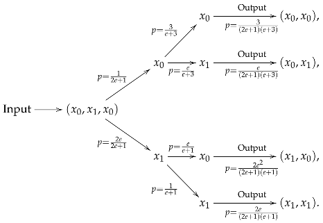
Example 1. 

Let $\mathbf{T}=\{e_0,e_1\}$ be the set of two tokens embedded in ${\mathbb{R}}^2$ such that $e_0=(1,0)$ and $e_1=(0,1).$ Then, $\mathbf{h}={\mathbb{C}}^2$ with the standard basis $|0⟩=|e_0⟩$ and $|1⟩=|e_1⟩.$ Let

$$\begin{array}{c}\hfill \mathbb{H}={\mathcal{F}}^{(3)}({\mathbb{C}}^2)=\mathbb{C}\oplus {\mathbb{C}}^2\oplus [{\mathbb{C}}^2\otimes {\mathbb{C}}^2]\oplus [{\mathbb{C}}^2\otimes {\mathbb{C}}^2\otimes {\mathbb{C}}^2].\end{array}$$

Suppose that $W^Q=W^K=\mathrm{FFN}=I$ in ${\mathbb{R}}^2$, and let $W^V={\sigma }_x,$ i.e., $W^V{e}_0=e_1$ and $W^V{e}_1=e_0.$ Below, we construct a quantum operation $\mathcal{E}$ associated with $\mathrm{SelfAtt}=(I,I,\sigma )$ and $\mathrm{FFN}=I$ in ${\mathbb{R}}^2.$ To this end, define $\mathsf{\Phi }(1)=|0⟩⟨0|,$

$$\begin{array}{c}\hfill \begin{array}{cc}\hfill \mathsf{\Phi }(|0⟩⟨0|)=& |0⟩⟨0| \times |W^V{e}_0⟩⟨W^V{e}_0|=|0⟩⟨0|\times |1⟩⟨1|,\hfill \\ \hfill \mathsf{\Phi }(|1⟩⟨1|)=& |1⟩⟨1| \times |W^V{e}_1⟩⟨W^V{e}_1|=|1⟩⟨1|\times |0⟩⟨0|;\hfill \end{array}\end{array}$$

and

$$\begin{array}{c}\hfill \begin{array}{cc}\hfill \mathsf{\Phi }(|0⟩⟨0|\otimes |0⟩⟨0|)=& |0⟩⟨0|\times |0⟩⟨0|\times |1⟩⟨1|,\hfill \\ \hfill \mathsf{\Phi }(|0⟩⟨0|\times |1⟩⟨1|)=& {\displaystyle \frac{e}{1+e}}|0⟩⟨0|\times |1⟩⟨1|\times |0⟩⟨0|\hfill \\ & +{\displaystyle \frac{1}{1+e}}|0⟩⟨0|\times |1⟩⟨1|\times |1⟩⟨1|,\hfill \\ \hfill \mathsf{\Phi }(|1⟩⟨1|\otimes |0⟩⟨0|)=& {\displaystyle \frac{1}{1+e}}|1⟩⟨1|\times |0⟩⟨0|\times |0⟩⟨0|\hfill \\ & +{\displaystyle \frac{e}{1+e}}|1⟩⟨1|\times |0⟩⟨0|\times |1⟩⟨1|,\hfill \\ \hfill \mathsf{\Phi }(|1⟩⟨1|\otimes |1⟩⟨1|)=& |1⟩⟨1|\times |1⟩⟨1|\times |0⟩⟨0|.\hfill \end{array}\end{array}$$

We regard $1,|e_i⟩⟨e_i|,$ $|e_j⟩⟨e_j|\otimes |e_k⟩⟨e_k|$ ($i,j,k=0,1$) as elements in $\mathcal{L}({\mathcal{F}}^{(3)}({\mathbb{C}}^2))$ in a natural way. Let

$$\begin{array}{c}\hfill \mathbf{S}=\mathrm{span}\{1,|e_i⟩⟨e_i|,|e_j⟩⟨e_j|\otimes |e_k⟩⟨e_k|:i,j,k=0,1\}.\end{array}$$

Then $\mathbf{S}$ is a subspace of $\mathcal{L}({\mathcal{F}}^{(3)}({\mathbb{C}}^2))$ and Φ extends uniquely to a positive map $\mathcal{E}$ from $\mathbf{S}$ into $\mathcal{L}({\mathcal{F}}^{(3)}({\mathbb{C}}^2)),$ i.e.,

$$\begin{array}{c}\hfill \begin{array}{cc}\hfill \mathcal{E}(a& +\sum _{i=0,1}{b}_i|e_i⟩⟨e_i|+\sum _{j,k=0,1}{c}_{j,k}|e_j⟩⟨e_j|\otimes |e_k⟩⟨e_k|)\hfill \\ \hfill =& a|0⟩⟨0|+\sum _{i=0,1}{b}_i\mathsf{\Phi }(|e_i⟩⟨e_i|)+\sum _{j,k=0,1}{c}_{j,k}\mathsf{\Phi }(|e_j⟩⟨e_j|\otimes |e_k⟩⟨e_k|),\hfill \end{array}\end{array}$$

for any $a,b_i,c_{j,k}\in \mathbb{C}.$ As shown in Proposition 3, $\mathcal{E}$ can extend to a completely positive operator in $\mathcal{L}({\mathcal{F}}^{(3)}({\mathbb{C}}^2)),$ which is a quantum operation in $\mathbb{H}={\mathcal{F}}^{(3)}({\mathbb{C}}^2)$ associated with $\mathrm{SelfAtt}=(I,I,\sigma )$ and $\mathrm{FFN}=I$ in ${\mathbb{R}}^2.$ Note that $\mathcal{E}$ is not necessarily unique.

Example 2. 

As in Example 1, $\mathbf{T}=\{x_0,x_1\}$ is the set of two tokens embedded in ${\mathbb{R}}^2$ such that $x_0=(1,0)$ and $x_1=(0,1).$ Then $\mathbf{h}={\mathbb{C}}^2$ with the standard basis $|0⟩=|x_0⟩$ and $|1⟩=|x_1⟩.$ Let $\mathbb{H}={\mathcal{F}}^{(6)}({\mathbb{C}}^2).$ Assume an input text $T=(x_0,x_1,x_0).$ The input state ${\rho }_T$ is then given by

$$\begin{array}{c}\hfill {\rho }_T=\rho (t_0)=\mathrm{diag}(0,0^{(1)},0^{(2)},|x_0⟩⟨x_0|\otimes |x_1⟩⟨x_1|\otimes |x_0⟩⟨x_0|,0^{(4)},0^{(5)},0^{(6)}).\end{array}$$

If $W_1^Q=W_1^K={\mathrm{FFN}}_1=I$ and $W_1^V={\sigma }_x$ in ${\mathbb{R}}^2,$ an associated physical operation $\mathcal{E}(t_1,t_0)$ at time $t_1$ satisfies

$$\begin{array}{c}\hfill \begin{array}{cc}\hfill \mathcal{E}(t_1,t_0)\rho (t_0)=& {\displaystyle \frac{1}{2e+1}}\mathrm{diag}(0,0^{(1)},0^{(2)},0^{(3)},|x_0⟩⟨x_0|\otimes |x_1⟩⟨x_1|\otimes |x_0⟩⟨x_0|\otimes |x_0⟩⟨x_0|,0^{(5)},0^{(6)})\hfill \\ \hfill +& {\displaystyle \frac{2e}{2e+1}}\mathrm{diag}(0,0^{(1)},0^{(2)},0^{(3)},|x_0⟩⟨x_0|\otimes |x_1⟩⟨x_1|\otimes |x_0⟩⟨x_0|\otimes |x_1⟩⟨x_1|,0^{(5)},0^{(6)}).\hfill \end{array}\end{array}$$

By measurement, we obtain $x_0$ with probability ${\displaystyle \frac{1}{2e+1}}$ and obtain $x_1$ with probability ${\displaystyle \frac{2e}{2e+1}},$ while

$$\begin{array}{c}\hfill \begin{array}{cc}\hfill {\rho }_{\mathrm{red}}{(t_1)}_0=& \mathrm{diag}(0,0^{(1)},0^{(2)},0^{(3)},|x_0⟩⟨x_0|\otimes |x_1⟩⟨x_1|\otimes |x_0⟩⟨x_0|\otimes |x_0⟩⟨x_0|,0^{(5)},0^{(6)}),\hfill \\ \hfill {\rho }_{\mathrm{red}}{(t_1)}_1=& \mathrm{diag}(0,0^{(1)},0^{(2)},0^{(3)},|x_0⟩⟨x_0|\otimes |x_1⟩⟨x_1|\otimes |x_0⟩⟨x_0|\otimes |x_1⟩⟨x_1|,0^{(5)},0^{(6)}).\hfill \end{array}\end{array}$$

If $W_2^Q=W_2^V={\mathrm{FFN}}_2=I$ and $W_2^K={\sigma }_x$ in ${\mathbb{R}}^2,$ an associated quantum operation $\mathcal{E}(t_2,t_0)$ at time $t_2$ satisfies

$$\begin{array}{c}\hfill \begin{array}{cc}\hfill \mathcal{E}(t_2,& t_0){\rho }_{\mathrm{red}}{(t_1)}_0\hfill \\ \hfill =& {\displaystyle \frac{3}{e+3}}(0,0^{(1)},0^{(2)},0^{(3)},0^{(4)},|x_0⟩⟨x_0|\otimes |x_1⟩⟨x_1|\otimes |x_0⟩⟨x_0|\otimes |x_0⟩⟨x_0|\otimes |x_0⟩⟨x_0|,0^{(6)})\hfill \\ & +{\displaystyle \frac{e}{e+3}}(0,0^{(1)},0^{(2)},0^{(3)},0^{(4)},|x_0⟩⟨x_0|\otimes |x_1⟩⟨x_1|\otimes |x_0⟩⟨x_0|\otimes |x_0⟩⟨x_0|\otimes |x_1⟩⟨x_1|,0^{(6)}),\hfill \end{array}\end{array}$$

and

$$\begin{array}{c}\hfill \begin{array}{cc}\hfill \mathcal{E}(t_2,& t_0){\rho }_{\mathrm{red}}{(t_1)}_1\hfill \\ \hfill =& {\displaystyle \frac{e}{e+1}}(0,0^{(1)},0^{(2)},0^{(3)},0^{(4)},|x_0⟩⟨x_0|\otimes |x_1⟩⟨x_1|\otimes |x_0⟩⟨x_0|\otimes |x_1⟩⟨x_1|\otimes |x_0⟩⟨x_0|,0^{(6)})\hfill \\ & +{\displaystyle \frac{1}{e+1}}(0,0^{(1)},0^{(2)},0^{(3)},0^{(4)},|x_0⟩⟨x_0|\otimes |x_1⟩⟨x_1|\otimes |x_0⟩⟨x_0|\otimes |x_1⟩⟨x_1|\otimes |x_1⟩⟨x_1|,0^{(6)}).\hfill \end{array}\end{array}$$

By measurement at time $t_2,$ when $x_0$ occurs at $t_1,$ we obtain $x_0$ with probability ${\displaystyle \frac{3}{e+3}}$ and obtain $x_1$ with probability ${\displaystyle \frac{e}{e+3}};$ when $x_1$ occurs at $t_1,$ we obtain $x_0$ with probability ${\displaystyle \frac{e}{e+1}}$ and obtain $x_1$ with probability ${\displaystyle \frac{1}{e+1}}.$

Therefore, we obtain the joint probability distributions:

$$\begin{array}{c}\hfill \begin{array}{cc}\hfill P_T(x_0,x_0)=& {\displaystyle \frac{1}{2e+1}}{\displaystyle \frac{3}{e+3}}={\displaystyle \frac{3}{(2e+1)(e+3)}},\hfill \\ \hfill P_T(x_0,x_1)=& {\displaystyle \frac{1}{2e+1}}{\displaystyle \frac{e}{e+3}}={\displaystyle \frac{e}{(2e+1)(e+3)}},\hfill \\ \hfill P_T(x_1,x_0)=& {\displaystyle \frac{2e}{2e+1}}{\displaystyle \frac{e}{e+1}}={\displaystyle \frac{2e^2}{(2e+1)(e+1)}},\hfill \\ \hfill P_T(x_1,x_1)=& {\displaystyle \frac{2e}{2e+1}}{\displaystyle \frac{1}{e+1}}={\displaystyle \frac{2e}{(2e+1)(e+1)}}.\hfill \end{array}\end{array}$$

This can be illustrated as follows:

6. Conclusions

Our primary innovative points are summarized as follows:

• Mathematical formalism for generative AI models. We present a mathematical formalism for generative AI models by using the theory of the history approach to physical systems developed by Isham and Gudder [1,2].
• Physical models realizing generative AI systems. We give a construction of physical models realizing generative AI systems as open quantum systems by using the theories of $\sigma$-effect algebras and open quantum systems.
• Large language models realized as open quantum system. We construct physical models realizing large language models based on the transformer architecture as open quantum systems in the Fock space over the Hilbert space of tokens. The Fock space structure plays a crucial role in this construction.

In conclusion, we present a mathematical formalism for generative AI and describe physical models realizing generative AI systems as open quantum systems. Our formalism shows that a transformer architecture used for generative AI systems is characterized by a family of sequential joint probability distributions. The physical models realizing generative AI systems are described by sequential event histories in open quantum systems. The Kraus operators in the physical models correspond to the query, key, and value matrices in the attention mechanism of a transformer, which are adjustable and learned during the training process. As an illustration, we construct physical models in the Fock space over the Hilbert space of tokens, realizing large language models based on a transformer architecture as open quantum systems. This means that our physical models underlie the transformer architecture for large language models. We refer to [23] for an argument on the physical principle of generic AI and to [15] for a mathematical foundation of general AI, including quantum AI.