A Deep Contextual Bandit-Based End-to-End Slice Provisioning Approach for Efficient Allocation of 5G Network Resources

Abstract

5G networks have been experiencing challenges in handling the heterogeneity and influx of user requests brought upon by the constant emergence of various services. As such, network slicing is considered one of the critical technologies for improving the performance of 5G networks. This technology has shown great potential for enhancing network scalability and dynamic service provisioning through the effective allocation of network resources. This paper presents a Deep Reinforcement Learning-based network slicing scheme to improve resource allocation in 5G networks. First, a Contextual Bandit model for the network slicing process is created, and then a Deep Reinforcement Learning-based network slicing agent (NSA) is developed. The agent’s goal is to maximize every action’s reward by considering the current network state and resource utilization. Additionally, we utilize network theory concepts and methods for node selection, ranking, and mapping. Extensive simulation has been performed to show that the proposed scheme can achieve higher action rewards, resource efficiency, and network throughput compared to other algorithms.

1. Introduction

In recent years, the fifth generation of communication networks, or simply 5G, has been continuously reshaping the ICT landscape. Along with the advent of 5G and beyond technologies, many services have also emerged, including augmented and virtual reality, vehicle-to-everything communications, e-health, and smart homes. Due to this diversity of existing services, the International Telecommunication Union (ITU) has identified three major usage scenarios for 5G services, namely: Ultra-Reliable Low Latency Communications (uRLLC), Enhanced Mobile Broadband (eMBB), and Massive Machine Type Communications (mMTC) [1]. Each of these usage scenarios has specific requirements that distinguish the types of resources allocated for each service request. To be specific, adaptive and on-demand resource provisioning methods based on varying service request types are needed to meet user needs [2]. Moreover, it is essential to meet the various requirements of these services to provide end-users with the best quality of service (QoS) possible.

One of the critical technologies on 5G and beyond systems is network slicing (NS) [3]. NS refers to creating multiple virtual networks within a 5G physical infrastructure to constitute a physical network. This technology is made possible by Software-Defined Networking (SDN) [4] and Network Function Virtualization (NFV) [5]. Moreover, each slice in the network has certain network functions tailored to the different services required by users. A classification of these slices includes service, resource, and deployment-driven NS solutions [6]. Moreover, creating slices for specific services within the physical network also ensures that network resources are efficiently utilized or allocated throughout the system. Likewise, NScan be broken down into three major processes: slice creation, slice isolation, and slice management [7]. This categorization of NS processes is further expanded into slice monitoring, slice mapping, and slice provisioning, as discussed in [8].

Recently, NS has become the subject of most research related to 5G networks, as it can improve service delivery and QoS. For example, the work in [9] studied the management and allocation of radio access networks (RAN) resources focusing on its impact on uRLLC and eMBB slices. The authors proposed an intelligent decision-making technique to manage network traffic and allocate the required resources. The work in [10] enumerates several factors that affect the implementation of network slices. These include resource allocation, slice isolation, security, RAN virtualization, feature granularity, and end-to-end (E2E) slice orchestration. Sohaib et al. presented the applications of machine learning (ML) and artificial intelligence (AI) for NS solutions in [11]. Their paper listed various ML and AI algorithms, and applications for different NS use-cases such as mobility prediction and resource management. Reference [12] studied the challenges in slice admission and management. The work investigated network revenue, QoS, inter-slice congestion, and slice fairness and possible solutions through various slice admission strategies and optimization techniques. Ye et al. [13] investigated how the NS process can improve E2E QoS in 5G networks by proposing an NS framework through effective resource allocation. Two scenarios, including (1) radio resource slicing for heterogeneous networks (HetNets) and (2) bi-resource slicing for core networks, were investigated to evaluate the efficiency of the proposed framework.

Recent studies have also applied the growing popularity of Deep Learning techniques to NS scenarios. For example, in [14], a framework for NS called DeepSlice was developed to classify incoming network service requests as either uRLLC, eMBB, or mMTC requests using Deep Learning. Ideal network slices for slice requests are then provided based on the classification results, with additional efficient resource allocation and network traffic regulation. The same authors of DeepSlice have also presented Secure5G [15], a Deep Learning-based framework designed for secure E2E-NS. This framework uses Deep Learning to identify network security threats through an NS- as-a-service model. Furthermore, Abbas et al. [16] proposed an intent-based NS (IBNSlicing) framework that aims to manage RAN and core network resources by using Deep Learning effectively. The framework focuses more on the process of slice orchestration, with the primary goal of improving the data transfer rate.

To the best of our knowledge, resource allocation influences several ways, from service provisioning to traffic or congestion management and ultimately to the QoS delivered by the whole network. More importantly, there should be mechanisms for monitoring the network’s state and current resource utilization to ensure that it handles all service requests at any time. Moreover, handling these service requests should be service-oriented and specific to each request’s requirements. Based on the information mentioned above, it is evident that the efficient allocation of network resources through NS dramatically affects the overall performance of 5G networks. Most of the works mentioned have presented the issues and challenges regarding resource allocation in 5G networks. However, most of these works have not thoroughly studied the potential of utilizing deep reinforcement learning methods for NS and resource allocation. Furthermore, these works have not investigated the effect of NS and resource allocation on the network’s resource efficiency and throughput.

For these reasons, we propose a Deep Contextual Bandits-based approach to NS for the improved resource allocation within a 5G network. Our work mainly focuses on the E2E provision of network slices to maximize RE and throughput by implementing Deep Reinforcement Learning and Network Theory. To be specific, the contributions of this work are as follows:

• A NS scenario is modeled as a Contextual Bandit problem, and an attempt is made to solve such a problem using a Deep Reinforcement Learning approach. Moreover, a network slicing agent (NSA) is developed and trained to perform slice creation for each Network Slice Request (NSR). For each NSR sent to the network, the agent is trained to select the best possible network slice from options. Accordingly, the state of the network determines the agent’s action and the reward it receives. Furthermore, the proposed work uses the Upper Confidence Bound (UCB) strategy to solve the exploration vs. exploitation dilemma in reinforcement learning, encouraging the agent to balance exploration and exploitation, resulting in more options for each NSR.
• Network theory is used to model the 5G network and its components. The modeling process is done through a graph-based approach that includes mapping, attribute definition, association, and path estimation of network nodes. The node degree and betweenness centrality, which are essential values for identifying appropriate nodes, are calculated for node selection. In addition, a link mapping method based on the Edmonds–Karp method to calculate the maximum flow is proposed.
• Network states are defined for the simulation as the basis for reward calculation. This work also considers the network’s current computing capability, bandwidth, node utilization, and the length of every candidate network slice as Reward Influencing Factors (RIF). Additionally, weights are assigned to each RIF to determine how they influence the reward for each action based on the current state of the network.

The remainder of this work is detailed as follows: Section 2 discusses related works that have served as a basis for this study. Next, Section 3 presents the proposed NS approach in detail. Section 4 then discusses the simulation scenario and results. Finally, Section 5 presents the conclusions and plans concerning this study.

2. Review of Related Works

Various works regarding resource allocation through 5G NS have been published in recent years. Most of the examined works in this section have proposed novel solutions to the resource allocation problem in NS. As such, they have served as an apparent motivation for the formulation of the proposed scheme.

2.1. Resource Allocation in 5G Networks

The efficient allocation of network resources is critical in mobile communication networks. Since the network receives many requests at a given time, it should be able to handle these requests without compromising the provided QoS. Therefore, significant efforts are being put into developing techniques for optimal resource allocation through NS. The authors in [17] presented various resource allocation methods for different 5G network scenarios. These include optimization, game theory, auction theory, and machine learning methods. The study in [18] suggests that user assignment, network utility, and throughput play an essential role in formulating resource allocation methods. Furthermore, in [19], the authors emphasized optimal dynamic resource management and aggregation as crucial components for effective resource allocation in 5G networks.

2.2. Network Slicing Solutions in 5G Networks

This section discusses the existing works focused on implementing NS solutions. Guan et al. in [20] utilized complex network theory methods to develop a service-oriented deployment approach to E2E-NS. In their work, NSRs are provisioned with slices by selecting the network node with the most favorable node importance among all candidate nodes at each time step. The importance of the node is calculated based on its degree and centrality. In addition, the authors then perform shortest path estimation to map all the selected nodes and create a network slice. Moreover, different slice provisioning strategies have also been formulated for uRLLC, eMBB, and mMTC service requests. Sciancalepore et al. designed a network slice brokering agent named ONETS [21]. The primary goal of their work is the development of a slice admission framework based on the multi-armed bandit problem. Such work has shown an increase in service request acceptance and maximization of network multiplexing gains through rewards systems, outperforming conventional existing reinforcement learning algorithms in the process. In [22], Abidi et al. attempted to address a slice allocation problem brought about by a massive data influx in the network. They introduced a Glowworm Swarm-based Deer Hunting Optimization Algorithm (GS-DHOA) to perform slicing classification. Based on their results, the proposed method distinguished uRLLC, eMBB, and mMTC requests and provided the necessary slices with great accuracy compared to other candidate algorithms utilized in the simulations. The work in [23] proposed a NS strategy by implementing a multi-criteria decision-making (MCDM) method. The authors used a slice provisioning algorithm based on the VIKOR approach to solve a 5G core-network-slice-provisioning problem (5G-CNSP). They also used complex network theory and a two-stage heuristic approach. The MCDM process for node selection considered the computational capacity and bandwidth of the nodes, as well as the local and global node topologies as decision parameters. Based on their results, the authors concluded that the proposed slicing strategy provides high RE and acceptance rate in high network traffic while addressing network security requirements. Fossati et al. [24] proposed a multi-resource allocation protocol for resource distribution on multiple network tenants. Their work proposed an optimization framework named multi-resources network slicing or MURANES that is based on the ordered weighted average (OWA) operator. The proposed solution considers the congestion and demand for resources from tenants. Likewise, the authors formulated allocation rules for single and multi-resource allocation scenarios. Results indicated that the proposed framework could address the multi-resource allocation problem while considering traffic support and heterogeneous congestion. The work in [25] introduced a prediction-assisted adaptive network slice expansion algorithm utilizing the Holt–Winters (HW) prediction method. The authors aimed to predict various changes occurring within the network and then provide services through a VNF adaptive scaling strategy. Network slices were proactively deployed based on NSRs received using network traffic rate and available resource information as the main parameters. Moreover, implementing the proposed approach resulted in lower energy consumption rates and slice deployment costs within the network. Sun et al. in [25] developed a RAN slicing framework for 5G networks aimed at maximizing bandwidth utilization and ensuring network QoS at the same time. Their paper focused on slice admission for NSRs through a joint slice association and bandwidth allocation approach. Slice admission policies for QoS optimization and user admissibility were then formulated, which increased the number of served users with the improved bandwidth consumption. Li et al. in [26] presented an application of Deep Q-Learning with the E2E-NS. The proposed algorithm maximizes user access through RAN and core network slices through dynamic resource allocation. Results of the simulations showed that the proposed reinforcement learning approach yielded a higher number of user access in both delays constrained and rate constrained slices. A summary of the related works is provided in Table 1.

Table 1. A Summary of Related Work on Resource Allocation and Network Slicing.

Ref	Objective	Proposed Solution	Performance Metrics
[14]	Optimal slice selection and prediction for mobile devices and adaptive slice assignments in the case of network failures	A Deep Learning and machine learning-based network slicing scheme that analyzes and predicts network traffic patterns for optimal resource allocation	Slice prediction accuracy Slice utilization Slice Failure
[15]	Secure network slicing for user equipment access	A neural network-based network slicing model for proactive threat detection and elimination	Threat detection accuracy
[16]	Efficient slice management and resource allocation for RAN and CN	An intent-based network slicing framework for upper-level slice configuration and orchestration	Data rate Network throughput
[19]	Integration of Mobile Edge Computing (MEC) for efficient allocation of idle 5G mobile network resources in urban settings	A MEC-based 5G network resource allocation framework for aggregated idle network resources	Service rate (in terms of served and blocked requests)
[20]	Service-oriented network E2E slice mapping and deployment	A complex network theory-based slice mapping and creation with slice deployment policy formulation for eMBB, mMTC, and uRLLC use-cases	Resource efficiency Acceptance Ratio
[21]	Efficient online service request-to-network slice brokering while considering network resource availability	A multi-armed bandit-based slice brokering method for budgeted resource lock-up for 5G network tenants	Cumulative agent rewards Tenant selection ratio System utilization distribution
[22]	Efficient network slicing using machine learning and AI techniques	A Deep Belief Network and Neural Network-based network slice classification scheme with Glowworm Swarm-based parameter weight optimization	Learning percentage Accuracy Sensitivity Specificity Precision
[23]	Implementation of MCDM-based node ranking for effective slice provisioning	A VIKOR algorithm-based core-network-slice-provisioning approach to secure network slicing	Acceptance ratio Revenue-to-cost ratio Node utilization
[24]	multi-resource allocation while considering resource usage fairness and system efficiency	A multi-resource allocation framework based on the Ordered Weighted Average (OWA) operator for resource availability and user demand information aggregation	Resource utilization Fairness
[25]	Efficient slice deployment through cost and network energy reduction	A dynamic slice deployment through a prediction-assisted adaptive network slice algorithm using Holt–Winters (HW) prediction	Energy consumption Link utilization Total slicing cost
[26]	Service provisioning in RAN slices while ensuring QoS and optimal resource utilization	A unified RAN slice provisioning framework for maximization of bandwidth utilization with user QoS guarantee	UE admission rate Bandwidth consumption Algorithm running time11
[27]	RAN and CN resource allocation through E2E NS while considering access rate and delay service requirements	A proposed Deep Q-Network algorithm for E2E wireless resource allocation and service link mapping on 5G network slices	E2E Access rate

3. Proposed Work

This section discusses the details of the proposed Deep Contextual Bandit-based network slicing (DCB-NS) scheme. It starts with the presentation of the proposed system architecture (Section 3.1), followed by the Network Slice Request Model (Section 3.2), the discussion of the Node Selection and Slice Mapping Model (Section 3.3), and then the specifics of the proposed scheme (Section 3.4).

3.1. System Architecture

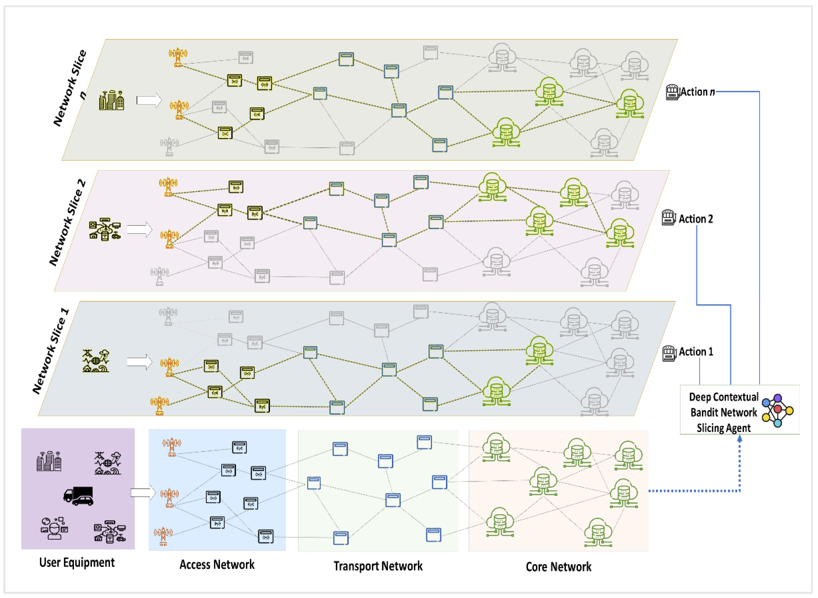
Figure 1 illustrates the system architecture of the proposed DCB-NS scheme. The proposed architecture divides the 5G network model into access, transport, and core networks. The main access point for users is through the access network. Next, the transport nodes forward service requests to the core network. Then, all service requests in the form of NSRs are processed in the core network, where the DCB-NS agent provisions appropriate network slices.

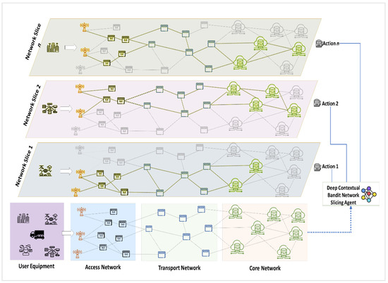
Figure 1. Proposed Deep Contextual Bandit 5G Network Slicing Architecture.

The proposed NS architecture consists of a set of physical nodes such as base stations, network switches, edge servers, and core computing servers $n=\left\{1,2,\dots ,N\right\}$, physical links $l=\{1,2,\dots ,L$} which are either wired or wireless, and user equipments $u=\left\{1,2,\dots ,U\right\}$. The network provides each node with a CPU computing capacity C. On the other hand, the network links are provided with link capacity B, measured in the allotted bandwidth per link. Lastly, the user equipments represent the devices (IoT devices, smartphones, and autonomous vehicles) that access and send NSRs to the 5G network.

3.2. Network Slice Request Model

The NSR of user $i$ at time $t$ is represented as $NS{R}_{i,t}=NS{R}^e\cup NS{R}^m\cup NS{R}^u$ with eMBB, mMTC, and uRLLC slice requests denoted by $NS{R}^e,NS{R}^m$, and $NS{R}^u$, respectively. For each slice request $NS{R}_{i,t}$, the user requests a specific amount of computing capacity $C_{NSR}$ (number of CPU cores) and link capacity $B_{NSR}$ (MHz) from the network based on the service or application they use. Additionally, each NSR includes the number of nodes $N_{NSR}$, a minimum transmission delay $D_{NSR}$ (milliseconds), the number of physical links (either wired or wireless) $L_{NSR}$, and the request lifetime $T_{NSR}$ (seconds) as request parameters. For example, we denote the uRLLC NSR for a user $U_{i,t}$ as $NS{R}^u{}_{i,t}=\left(C^u{}_{NSR},B^u{}_{NSR},N^u{}_{NSR},D^u{}_{NSR},L^u{}_{NSR},T^u{}_{NSR}\right)$. Furthermore, based on this model, the network will be able to identify the resources required by a user for each NSR and handle such requests by allocating the necessary resources through a network slice.

3.3. Node Selection and Slice Mapping Model

The node selection method is based on network theory [27,28] and uses node degree and centrality values to select candidate nodes for $NS{R}_{i,t}$. These parameters are chosen to select the nodes with the optimal position in the network. Accordingly, the degree of a node refers to the number of connections adjacent to other nodes in the network. Each node $n\in N$ has two degrees: an out-degree, which refers to the number of outgoing edges,

$$k_i^{in}={\displaystyle \sum }_{j=0}^J{\epsilon }_{j,i}$$

(1)

and an in-degree of the number of incoming edges onto $n$,

$$k_i^{out}={\displaystyle \sum }_{j=0}^J{\epsilon }_{i,j}$$

(2)

where $\epsilon$ is equal to 1 if node $i$ is directly connected to node $j$, and 0 if otherwise. The total degree of a node is then calculated as,

$${\displaystyle \sum }_{i=0}^I{k}_i=k_i^{in}+k_i^{out}$$

(3)

A centrality analysis is then performed for each node to determine its degree of importance to the information flow in the network. In this study, the betweenness centrality of the node is the chosen measure. We are interested in selecting candidate nodes based on how frequently they are used for network information flow. As such, the betweenness centrality of node i is estimated as,

$$\beta \left(n_i\right)={\displaystyle \sum }_{j=1}^J\frac{g_j\left(n_i\right)}{g_j}$$

(4)

where $g_j\left(n_i\right)$ is the number of all paths passing through node $n_i$, and $g_j$ is the sum of all the shortest paths from nodes $j$ to $k$.

The node’s viability $\xi$ is then calculated using the values for ${\displaystyle \sum }_{i=0}^I{k}_i$ and $\beta \left(n_i\right)$ as in Equation (5),

$$\xi =\frac{{{\displaystyle \sum }}_{i=1}^{I}C\left(n_i\right)\ast \left({{\displaystyle \sum }}_{i=1}^{L_{NSR}}B\left(n_i\right)\right)}{{{\displaystyle \sum }}_{i=0}^I{k}_i+\beta \left(n_i\right)}$$

(5)

where the node resource values ${\displaystyle \sum }_{i=1}^{I}C\left(n_i\right)$ for computing capacity, and ${\displaystyle \sum }_{i=1}^{L_{NSR}}B\left(n_i\right)$ for the total link capacity for all links of $n_i$ are considered. All ξ values are stored and arranged (in descending order) in the node viability array (NVA) to be used later for candidate node selection. Moreover, sorting from the highest value to the lowest means that nodes with higher $\xi$ values are given priority for candidate node selection (Algorithm 1).

Algorithm 1. NSR Node Selection Method.
1:	initialize $k_i^{in}$, $k_i^{out}$, $\beta \left(n_i\right)$, ${\displaystyle \sum }_{i=1}^{I}C\left(n_i\right)$, ${\displaystyle \sum }_{i=1}^{L_{NSR}}B\left(n_i\right)$, and x values
2:	for each node i with $C\left(n_i\right)>0$:
3:	calculate node degree ${\displaystyle \sum }_{i=0}^I{k}_i$ (Equation (3))
4:	calculate node betweenness centrality $\beta \left(n_i\right)$ (Equation (4))
5:	calculate node viability $\xi$ value (Equation (5))
6:	save $\xi$ of node $i$ to NVA
7:	sort NVA values in descending order
8:	for each $NS{R}_{i,t}$:
9:	input x value as the number of nodes to select from NVA
10:	while $x\ne 0$:
11:	retrieve ${\mathsf{\xi }}_x$ from NVA
12:	return ${\mathsf{\xi }}_x$ and perform node mapping (Algorithm 2)

For the mapping of paths that interconnect network nodes, conventional approaches use the shortest path methods [20,23,28] such as breadth-first search (BFS) and k-shortest path algorithms. This study implements the maximum flow approach utilizing the Edmonds–Karp method [29]. The network’s maximum flow indicates the amount of data that can flow through the network’s connections at a given time. This approach calculates the network’s flow by taking the sum of available bandwidth for all edges in the network. Additionally, this process aims to find all feasible paths or augmenting paths $\psi \left(n_{\alpha },n_{\mathsf{\Omega }}\right)$ from source node $n_{\alpha }$ to target node $n_{\mathsf{\Omega }}$ for every $NS{R}_{i,t}$ while considering the link capacity of every edge in the network. Such an approach reduces the chances of congestion when there is an influx of requests in the network. The nodes ranked in the NVA are used as target nodes for the link mapping process using the Edmonds–Karp method. Furthermore, choosing the best path for the selected nodes requires satisfying the following inequalities,

$${\psi }_{i,length}\le {\Psi }_{\mu }-1$$

(6)

$$f_{residual}\ge B_{NS{R}_{i,t}}$$

(7)

$$T_{round}\le T_{NSR}$$

(8)

where $f_{residual}$ is the total residual flow (in terms of link capacity) for path $i$ from the source node to the target node for $NS{R}_{i,t}$, ${\psi }_i^{length}$ is the length of path $i$, ${\Psi }_{\mu }$ is the average path length for all node connections, and $T_{round}$ is the total roundtrip time for data transmission from the source to target node expressed as,

$$T_{round}=T_{\left(n_{\alpha },n_{\mathsf{\Omega }}\right)}+T_{\left(n_{\mathsf{\Omega }},n_{\alpha }\right)}$$

(9)

where $T_{\left(n_{\alpha },n_{\mathsf{\Omega }}\right)}$ and $T_{\left(n_{\mathsf{\Omega }},n_{\alpha }\right)}$ refer to the transmission times from the source node to the target node, and from the target node to the source node, respectively. These transmission times denote the amount of time required for the NSR to travel from the source node to the target node (vice-versa) and is affected by transmission delays.

Algorithm 2 presents the details of the link mapping method. This approach aims to find the best path to the target node $n_{\mathsf{\Omega }}$ for $NS{R}_{i,t}$. Equation (6) ensures that the length of this path does not exceed the average length of all paths in the network. Equation (7) guarantees that the residual flow meets the required link capacity for $NS{R}_{i,t}$. In addition, Equation (8) ensures that the total time needed to transmit $NS{R}_{i,t}$ from $n_{\alpha }$ to $n_{\mathsf{\Omega }}$ (vice-versa) does not exceed the specified lifetime of the NSR. Furthermore, all identified augmenting paths are used as links for candidate network slices by the DCB-NS agent for NSR slice provisioning.

Algorithm 2. NSR Link Mapping Method.
1:	initialize flow value $f=0$
2:	for each ${\mathsf{\xi }}_x$ value from NVA:
3:	select source node $n_{\alpha }$ and initialize node of $n_{{\mathsf{\xi }}_x}$ as target node $n_{\Omega }$
4:	let $\psi {\left(n_{\alpha },n_{\mathsf{\Omega }}\right)}_{{\mathsf{\xi }}_x}\in G$ be a path with the minimum number of edges
5:	perform Breadth-First Search for $n_A$ to $n_{\mathsf{\Omega }}$
6:	for each $\mathrm{edge}\left(i,j\right)$ in $\left(\psi \right){\left(n_{\alpha },n_{\mathsf{\Omega }}\right)}_{{\mathsf{\xi }}_x}$:
7:	calculate for residual flow $f_{residual,i}$
8:	$f_{residual,i}=f\left(i,j\right)+c_{residual}\left(\psi \right){\left(n_{\alpha },n_{\mathsf{\Omega }}\right)}_{{\mathsf{\xi }}_x}$, for forward                  edges
9:	$f_{residual,i}=f\left(i,j\right)-c_{residual}\left(\psi \right){\left(n_{\alpha },n_{\mathsf{\Omega }}\right)}_{{\mathsf{\xi }}_x}$, if otherwise
10:	if Equations (6)–(8) = true:
11:	store $\left(\psi \right){\left(n_{\alpha },n_{\mathsf{\Omega }}\right)}_{{\mathsf{\xi }}_x}$ to augmenting path array $P_{aug}[]$
12:	select $\left(\psi \right){\left(n_{\alpha },n_{\mathsf{\Omega }}\right)}_{{\mathsf{\xi }}_x}$ with highest $f_{residual}$ from $P_{aug}[]$ as NSR path $\psi {\left(n_{\alpha },n_{\mathsf{\Omega }}\right)}_{NS{R}_{i,t}}$
13:	return $\psi {\left(n_{\alpha },n_{\mathsf{\Omega }}\right)}_{NS{R}_{i,t}}$

3.4. Deep Contextual Bandit Network Slicing Scheme

Reinforcement learning (RL) methods facilitate agent learning through evaluative feedback. An action performed by an agent is evaluated based on its quality, for which it receives a corresponding reward. In addition, RL agents attempt to solve a problem by balancing exploitation and exploration of actions. This process, in turn, allows the agent to learn a strategy to obtain an optimal reward for each action. Additionally, the way RL agents learn is in direct contrast to other AI methods that guide the agent to take corrective actions based on existing training data.

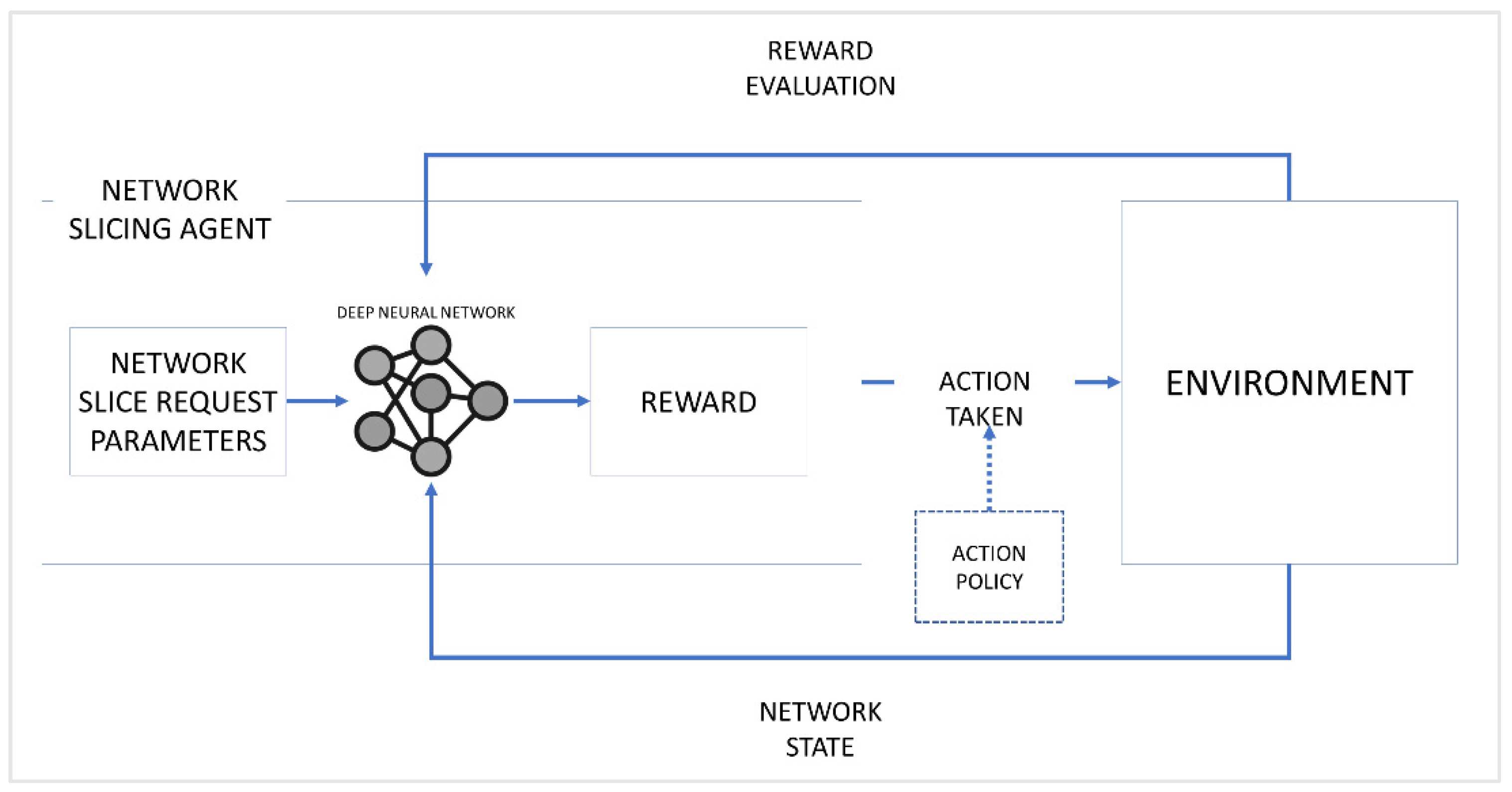
This work implements a variant of the multi-armed (or k-armed) bandit approach known as Contextual Bandits [30] for the proposed NS scheme. This approach is a type of associative search method in which the current state of the environment affects an agent’s reward for a given action. A famous example of this scenario is the case of slot machines in a casino, where a player tries to get the best payoff while playing slot machines. In this scenario, the rewards for pulling the arm of a slot machine (or bandit) are randomly distributed and are unknown to the player, so the player must choose the best action strategy to get the best payoff. Therefore, we model the proposed scheme based on a Contextual Bandit scenario. Moreover, a deep reinforcement learning is utilized to compute the reward and formulate the action strategy efficiently through a trial-and-error approach. The deep neural network receives the NSR parameters as through its input layer and then outputs it through the output layer. The rewards are calculated based on the network’s current state and checked for errors or losses using the mean squared error method. Such an approach leads to an optimal resource allocation strategy in the form of a network slice for each NSR. A graphical representation of the Deep RL model is shown in Figure 2.

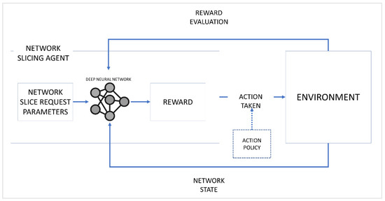
Figure 2. Deep Reinforcement Learning Model for the proposed work.

The proposed scheme considers an input $\eta$, and a set of actions $A$, and each action $a\in A$ has an associated reward $R_t$. In this case, $NS{R}_{i,t}$ and the mapped nodes $\psi {\left(n_{\alpha },n_{\mathsf{\Omega }}\right)}_{NS{R}_{i,t}}$ represent the input and the agent’s actions, respectively. For every action taken, the agent expects to achieve a value or utility $q_{\ast }\left(a\right)$ that measures the quality of such action. This value or utility calculation is expressed as,

$$q_{\ast }\left(a\right)=E\left[R_t|A_t=a\right]$$

(10)

thus, the expected value $q_{\ast }\left(a\right)$ for action $a$ is equivalent to the reward for that action at time $t$. In addition, the actions in the agent’s action space are randomly distributed using a Softmax function, which is denoted as,

$$\sigma {\left(z\right)}_i=\frac{ex{p}^{z_i}}{{{\displaystyle \sum }}_{j=1}^{K}ex{p}^{z_j}}$$

(11)

where the probability of choosing an action is calculated by dividing the input vector’s exponential function $ex{p}^{z_i}$ over the sum of all the exponential functions for an output vector $ex{p}^{z_j}$ for a $K$ number of classes. Moreover, this probability distribution method enables the NSA to randomly select an action out of a given set of possible actions without any bias.

Since the Contextual Bandit approach considers the environment state to determine the reward for an action taken, it is also necessary to define state $S$ as a set of states where each state $s\in S$ comprises various reward influencing factors (RIF). The various factors are defined as follows:

1.

The total path length $L_{hops}$ is the sum of all paths from $n_{\alpha }$ to $n_{\mathsf{\Omega }}$. This value provides the agent with the candidate slice topology information.

$$L_{hops}={\displaystyle \sum }_{i=0}^{n_{\mathsf{\Omega }}}\mathsf{\psi }\left(n_i\right)$$

(12)

2.

The computing capacity utilization denoted as $C_{\delta }$ provides information regarding the computing capacity ${\displaystyle \sum }_{i=1}^I{C}_{NS{R}_i}$ allocated for $NS{R}_i$ at time $t$. This value also helps determine the remaining computing capacity for the network’s physical infrastructure at the specified time step.

$$C_{\delta }=\frac{{{\displaystyle \sum }}_{i=1}^I{C}_{NS{R}_i}}{{{\displaystyle \sum }}_{n=1}^N{C}_n}$$

(13)

where ${\displaystyle \sum }_{n=1}^N{C}_n$ refers to the total remaining computing capacity for all physical infrastructure nodes.

3.

The bandwidth utilization $B_{\delta }$ reflects the network’s total bandwidth utilized at time $t$. This bandwidth utilization is also affected by other NSRs served at the specified time step.

$$B_{\mathsf{\delta }}=\frac{{{\displaystyle \sum }}_{i=1}^I{B}_{NS{R}_i}}{{{\displaystyle \sum }}_{i=1}^L{B}_i}$$

(14)

where ${\displaystyle \sum }_{i=1}^I{B}_{NS{R}_i}$ is the allocated link capacity for $NS{R}_i$ and ${\displaystyle \sum }_{i=1}^L{B}_i$ is the total remaining link capacity for all nodes from the physical infrastructure.

4.

Node utilization $N_{\rho }$ represents the percentage of network nodes serving all existing NSRs at time $t$. It also verifies whether the network can allocate the nodes needed by the NSR.

$$N_{\rho }=\frac{{{\displaystyle \sum }}_{i=1}^I{N}_{NS{R}_i}}{{{\displaystyle \sum }}_{n=1}^N{N}_n}$$

(15)

where ${\displaystyle \sum }_{i=1}^I{N}_{NS{R}_i}$ is the number of allocated nodes for $NS{R}_i$ at time $t$ and ${\displaystyle \sum }_{n=1}^N{N}_n$ is the total remaining number of physical infrastructure nodes.

Using RIFs as weights whose values are determined by the network state, the reward $R_i$ for action $a_i$ is calculated as

$$R_i=\mathsf{\sigma }\left(a\right)·\left(\frac{\left(w_1\right)L_{hops}+\left(w_2\right)C_{\delta }+\left(w_3\right)B_{\delta }+\left(w_4\right)N_{\rho }}{\left({{\displaystyle \sum }}_{n=1}^N{C}_n+{{\displaystyle \sum }}_{i=1}^L{B}_i+{{\displaystyle \sum }}_{n=1}^N{N}_n\right)\ast L_{hops}}\right)$$

(16)

where $w\in \left[0,1\right]$ is a weight factor defined by the network’s current state. We have defined the following network states $s_t$ to find for reward $R_i$ as follows:

1.

Network State 1 ($S_1$) represents a normal network state, meaning that the total available computing capacity ${\displaystyle \sum }_{n=1}^N{C}_n$, link capacity ${\displaystyle \sum }_{i=1}^L{B}_i$, the number of usable nodes ${\displaystyle \sum }_{n=1}^N{N}_n$, and total path length $L_{hops}$ are at 81–100%.

2.

Network State 2 ($S_2$) indicates that ${\displaystyle \sum }_{n=1}^N{C}_n$, ${\displaystyle \sum }_{i=1}^L{B}_i$, ${\displaystyle \sum }_{n=1}^N{N}_n$, and $L_{hops}$ are at 50–80% capacity or availability. Such a state requires that succeeding NSRs should not exceed the remaining capacity of available network resources.

3.

Network State 3 ($S_3$) signals that all network resources are below 50% capacity or availability. This state indicates either that the network is currently serving many NSRs or the NSRs currently served are utilizing a large amount of resource capacity.

Based on these network states, a combination of values for each $w$ of a RIF is assigned in Table 2.

Table 2. Weight value assignment for RIFs based on the network state $s_t$.

${\mathit{w}}_{\mathit{i}}$  ${\mathit{s}}_{\mathit{i}}$	${\mathit{w}}_1$	${\mathit{w}}_2$	${\mathit{w}}_3$	${\mathit{w}}_4$
$s_1$	0.50	0.75	0.75	0.50
$s_2$	0.50	1	1	0.75
$s_3$	1	1	1	1

The weight assignments in Table 2 show that $s_3$ requires a careful allocation of resources for an NSR to avoid network failure. State $s_2$, on the other hand, prioritizes resource allocation for computing capacity and bandwidth to incoming NSRs. Finally, $s_1$ has a lower priority on resource allocation since the network has high resource availability.

Next, the accumulated reward for a specific action $a$ at time $t$ is denoted as $Q_t\left(a\right)$ and then calculated after exploring all possible actions from the action space as,

$$Q_t\left(a\right)=\frac{1}{y}{\displaystyle \sum }_{i=1}^y{R}_i$$

(17)

where $y$ is the number of instances performed by the agent for action $a$, and $R_i$ is the reward earned for each action.

The Upper Confidence Bound (UCB) strategy is utilized to facilitate the exploration and exploitation of actions. Through this, the agent decides whether to continue choosing an action that gives a particular reward value (exploitation) or to check for other possible actions that could yield higher rewards (exploration). The UCB for action $a_i$ is expressed as follows,

$$UCB={\mathrm{argmax}}_a\left[Q_t\left(a\right)+c\sqrt{\frac{\log \left(t\right)}{Y_{t\left(a\right)}}}\right]$$

(18)

where $Y_t\left(a\right)$ is the number of instances when action $a$ is chosen before time $t$, and $c$ is a predefined confidence value controlling the degree of exploration. The UCB strategy implies that by checking each action’s $Q_t\left(a\right)$ and the number of instances it was executed, it can exploit the action with the highest $UCB$. However, other possible actions are explored and re-evaluated.

The calculated rewards are then evaluated for every action the agent performs to assess its quality. At the end of the training period, the cumulative mean rewards $q_{\ast }{\left(a\right)}_{\mathsf{\mu }}$ for each action are taken as,

$$q_{\ast }{\left(a\right)}_{\mathsf{\mu }}=\frac{{{\displaystyle \sum }}_{a=0}^A{Q}_{t\left(a\right)}}{Y_a}$$

(19)

where Y denotes the number of instances when the agent chose action $a_i$. These values are then ranked in descending order, and the action with the highest $q_{\ast }\left(a\right)s_{\mathsf{\mu }}$ is implemented as a network slice $N{S}_{NS{R}_{i,t}}$. Finally, the proposed DCB-NS scheme details are presented in Algorithm 3.

Algorithm 3. Proposed Deep Contextual Bandit Network Slicing Scheme.
1:	initialize $NS{R}_{i,t}=\left(C_{NSR},B_{NSR},N_{NSR},D_{NSR},L_{NSR},T_{NSR}\right)$, $x$, $y$, $c$
2:	perform Node Selection (Algorithm 1)
3:	for x in NVA:
4:	perform Node Mapping (Algorithm 2)
5:	add mapped nodes to candidate slices array $Slices[]$
6:	check for network state $s_t$
7:	while $y>0$:
8:	select action a candidate slice from Slices[] as action $a_i$
9:	calculate action value $q_{\ast }\left(a\right)$ (Equation (10))
10:	calculate reward $R_i$ (Equation (16))
11:	calculate total estimated value $Q_t\left(a\right)$ (Equation (17))
12:	calculate Upper Confidence Bound $UCB$ (Equation (18))
13:	if $length\left(A\right)$ = 1:
14:	set $UCB$ of $a_i$ as the max UCB
15:	select new action $a_{i+1}$, repeat steps 8–12
16:	else: Compare $UCB$ values for all actions performed
17:	if $UCB$ of current action is highest:
18	set $UCB$ of that action as max UCB (exploit)
19:	else: select new action and repeat from step 8 (explore)
20:	select action with the highest $q_{\ast }{\left(a\right)}_{\mu }$ from all actions performed in $a\in A$
21:	implement selected action as network slice $N{S}_{NS{R}_{i,t}}$ for $NS{R}_{i,t}$
22:	return $N{S}_{NS{R}_{i,t}}$

4. Simulation Environment and Performance Metrics

4.1. Simulation Environment Configuration

Table 3 shows the simulation configurations. The network setup assumes 100–300 nodes for the physical infrastructure. These nodes are then divided into the access, transport, and core network nodes. For the node computing and link capacity, a range of 20 to 50 are assumed. For every NSR, a total of 15 nodes, computing and link capacity within 5 to 25, transmission delay of 0.05 to 1, and NSR lifetime of 10 to 50 are assigned. In addition, the number of NSRs that are simultaneously served is limited to 20 NSRs.

Table 3. Simulation Configurations.

Parameter	Range
Physical Network:
Access network nodes	20, 40, 80
Transport network nodes	30, 60, 120
Core network nodes	50, 100, 200
Node computing capacity	U [20, 50]
Node link capacity	U [20, 50]
Network Slice Requests:
Number of nodes per NSR	15
Maximum number of NSRs	20
NSR node computing capacity	U [5, 25]
NSR link capacity	U [5, 25]
Transmission Delay	T [0.05, 1]
NSR Lifetime	T [10, 50]

Since the proposed scheme implements Deep RL, the properties of the deep neural network are defined as follows: a sequential model where each layer uses a linear transformation, rectifier linear unit (ReLU) as the activation function, Adam as the optimizer, and mean squared error (MSE) for loss calculation.

4.2. Performance Metrics

The proposed scheme’s performance evaluation includes assessing the network’s resource efficiency (RE) and throughput. The RE is defined based on how the network allocates resources to each slice requested by the NSR. Ideally, the network should effectively allocate the requested resources without exhausting most of the physical infrastructure resources. As such, the network’s RE is expressed as,

$$\mathsf{\phi }=\frac{{{\displaystyle \sum }}_{i=1}^I{C}_{NS{R}_i}+{{\displaystyle \sum }}_{i=1}^I{B}_{NS{R}_i}+{{\displaystyle \sum }}_{i=1}^I{N}_{NS{R}_i}}{\left(C_{\mathsf{\delta }}+B_{\mathsf{\delta }}+N_{\mathsf{\delta }}\right)\ast L_{hops}}$$

(20)

The network throughput measures the ratio of all NSRs served to the total number of NSRs received at time $t$. The network must serve all requested network slices by effectively allocating resources to achieve the highest possible throughput at each time step. The network’s throughput is calculated as,

$$\mathsf{\Gamma }=\frac{{{\displaystyle \sum }}_{t=0}^{T}NS{R}_{served,t}}{{{\displaystyle \sum }}_{t=0}^{T}NS{R}_{received,t}}$$

(21)

Additionally, the proposed scheme utilizes the cumulative mean rewards (Equation (19)) earned for performance evaluation as an additional metric.

5. Results and Discussions

The proposed DCB-NS scheme compares its performance with the Epsilon–Greedy and Thompson sampling algorithms [31]. Together with UCB (which the proposed scheme utilizes), these algorithms are popular approaches for solving multi-armed bandit problems. The proposed scheme is first evaluated based on the cumulative rewards obtained by the agent using the three methods above. Then, the effectiveness of the proposed scheme through network slice provisioning for each NSR is evaluated. In addition, the throughput of the network is examined to determine how well it serves the incoming NSRs during the simulation period. In this section, the results of the simulations are presented and discussed.

5.1. Agent Rewards Accumulation

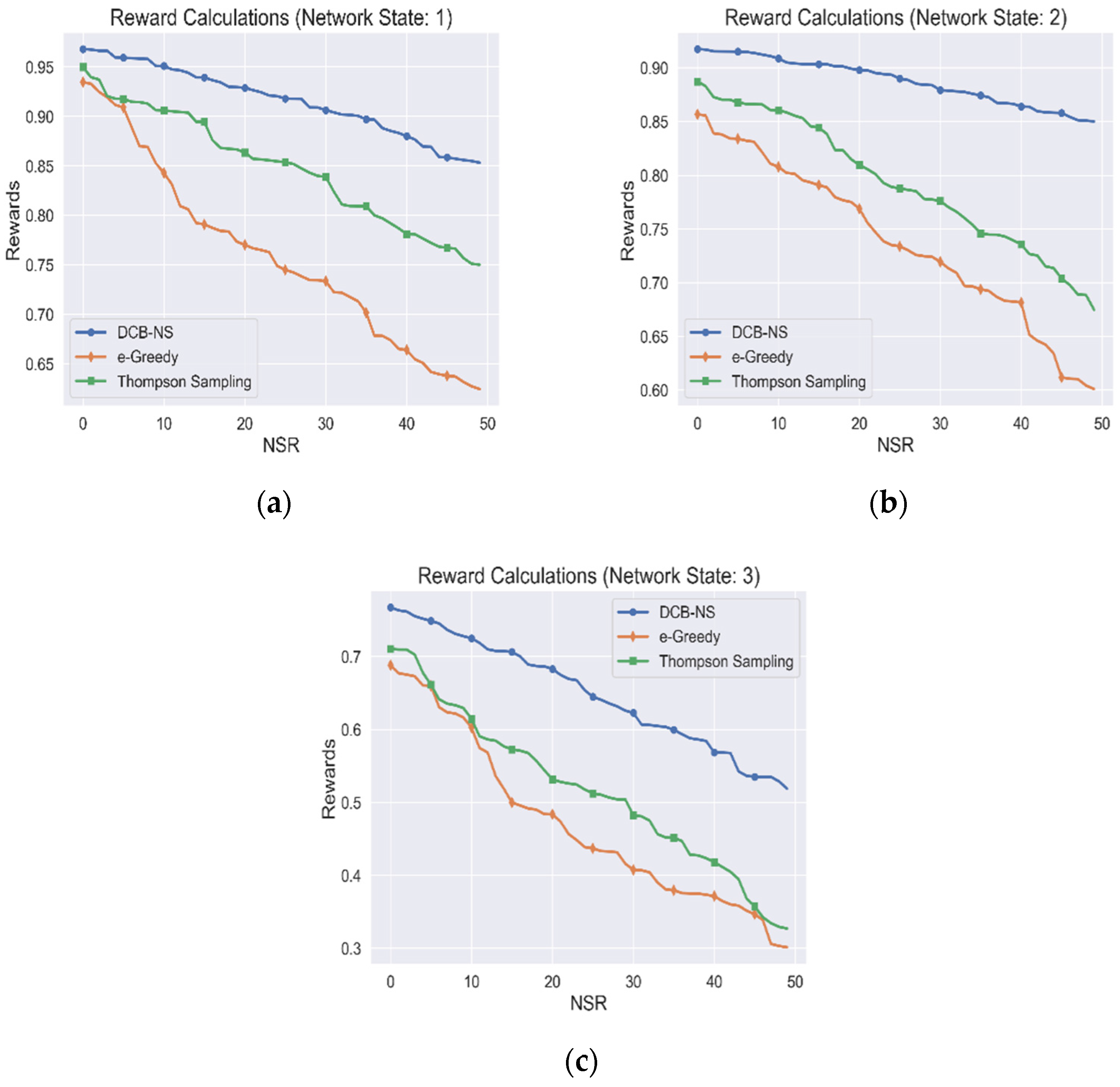
The rewards accumulated by the NSA from the simulations are shown in Figure 3. The proposed scheme is evaluated based on network states 1, 2, and 3, as shown in Figure 3a–c, respectively. The simulation is implemented using a total node value of 300 for maximum resource distribution. Additionally, for this simulation, we have only taken the rewards gained for all optimal actions chosen, which resulted in creating a network slice for an NSR.

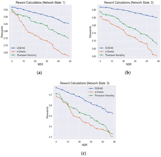
Figure 3. Cumulative Agent Rewards for (a) Network State 1, (b) Network State 2, and (c) Network State 3.

Based on the results, it can be observed that the rewards earned by the agent gradually decrease as the number of NSRs received by the network increases. This decline in rewards is due to the increase in resource utilization of the network, which affects the RIFs used for the reward calculation.

Similarly, the previously defined network states are essential indicators of the current resource availability in the network. Moreover, it is observed that the upper bound for the maximum reward also decreases due to this condition. However, unlike the other two algorithms, the DCB-NS strategy achieves higher rewards. This advantage is due to the efficiency of the UCB strategy in selecting the ideal actions by evaluating their confidence value, which increases the certainty of higher incentives for each scenario. On the other hand, Thompson sampling leads to an unbalanced distribution of actions due to the random nature of the sampling process, which is in contrast to the consistent performance of UCB [32]. Moreover, the algorithm is likely to become unstable during extended training periods. The Epsilon–Greedy algorithm achieves the lowest rewards because it simply relies on the randomness of the Epsilon value to balance exploration and action utilization [22]. Moreover, this algorithm explores only the neighboring solutions once an inferred distribution is known, leading to inefficient action policies. This property contrasts with the uniform distribution of action probabilities of the proposed scheme using the Softmax function, which ensures a higher likelihood of action exploration.

5.2. Network Resource Efficiency

Next, a simulation is performed to evaluate the efficiency of network resources (RE) in serving the received NSRs. Figure 3 and Figure 4 show the results considering the maximum number of nodes and the network states.

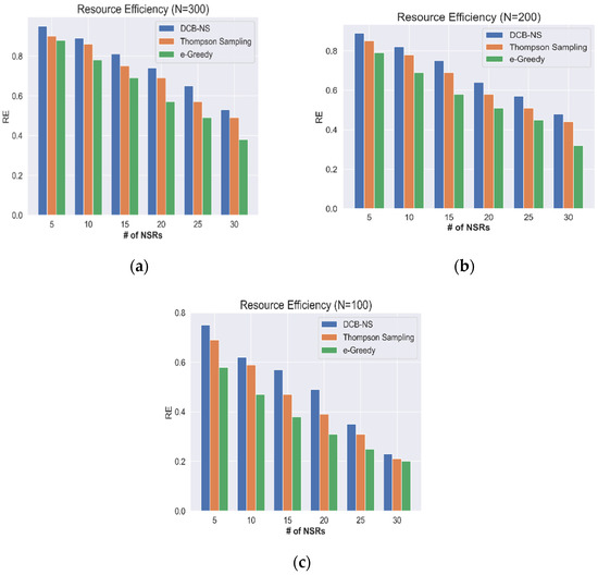
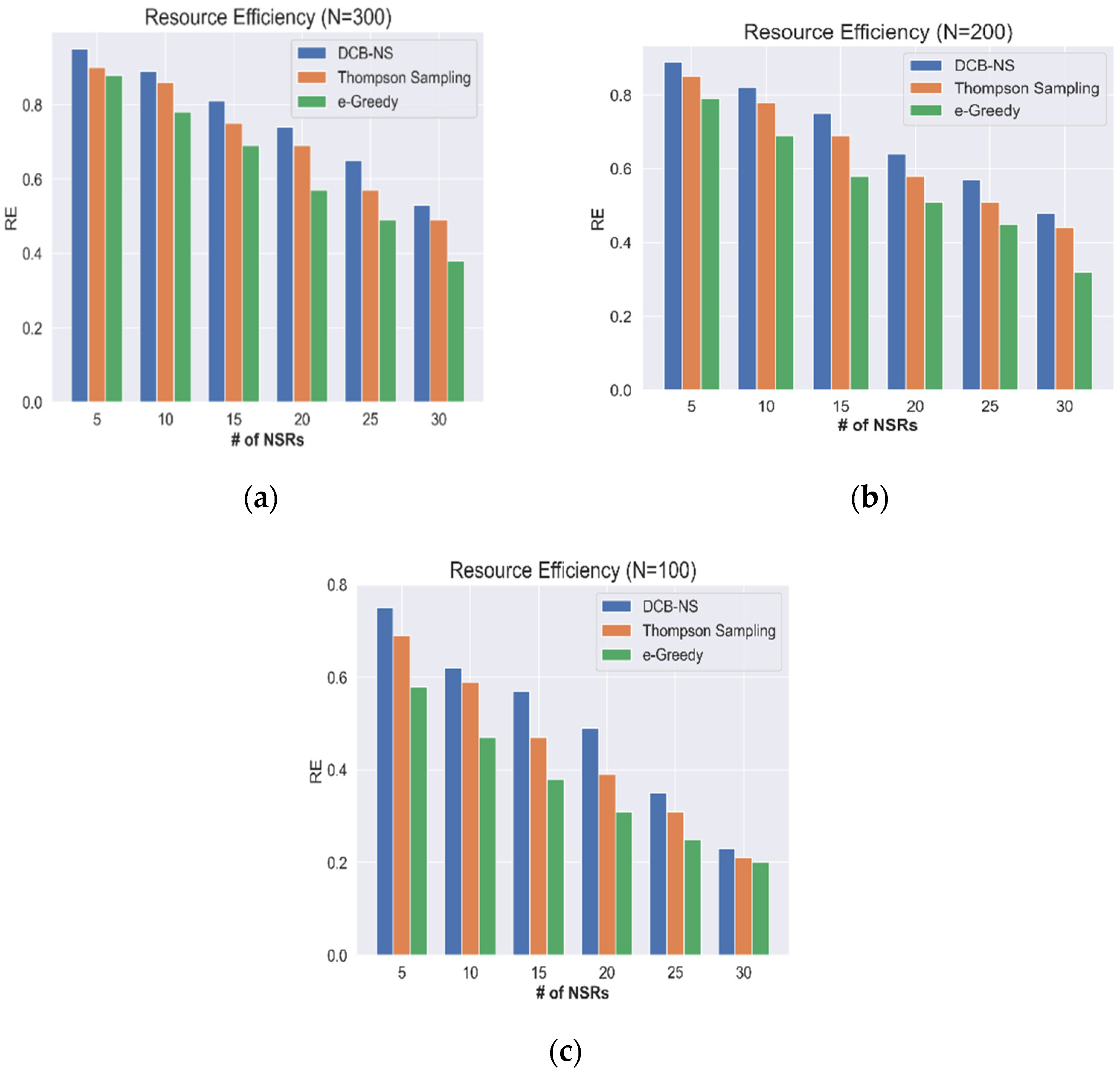
Figure 4. Network Resource Efficiency according to the maximum number of nodes: (a) N = 300, (b) N = 200, and (c) N = 100.

The RE calculated based on the total number of nodes (100, 200, 300), are shown in Figure 4. At N = 300, the network can maintain a value above the median for RE, although the resource availability gradually decreases as the number of NSRs increases. In contrast, the network encounters resource shortages when N = 100, leading to a sharp decline in RE when the number of NSRs peaks. Therefore, effective network resource allocation schemes are required to keep the network operational regardless of the surge of service requests. During simulations, the proposed DCB-NS scheme has maintained a higher RE than the Thompson Sampling and Epsilon–Greedy methods. The proposed scheme improves the slice allocation process by utilizing the RIF values that determine the current network resource utilization. Additionally, the integrated maximum flow computation ensures an efficient mapping of network slices. These processes allow the NSA to intelligently select the best possible network slices by considering the current state of the network.

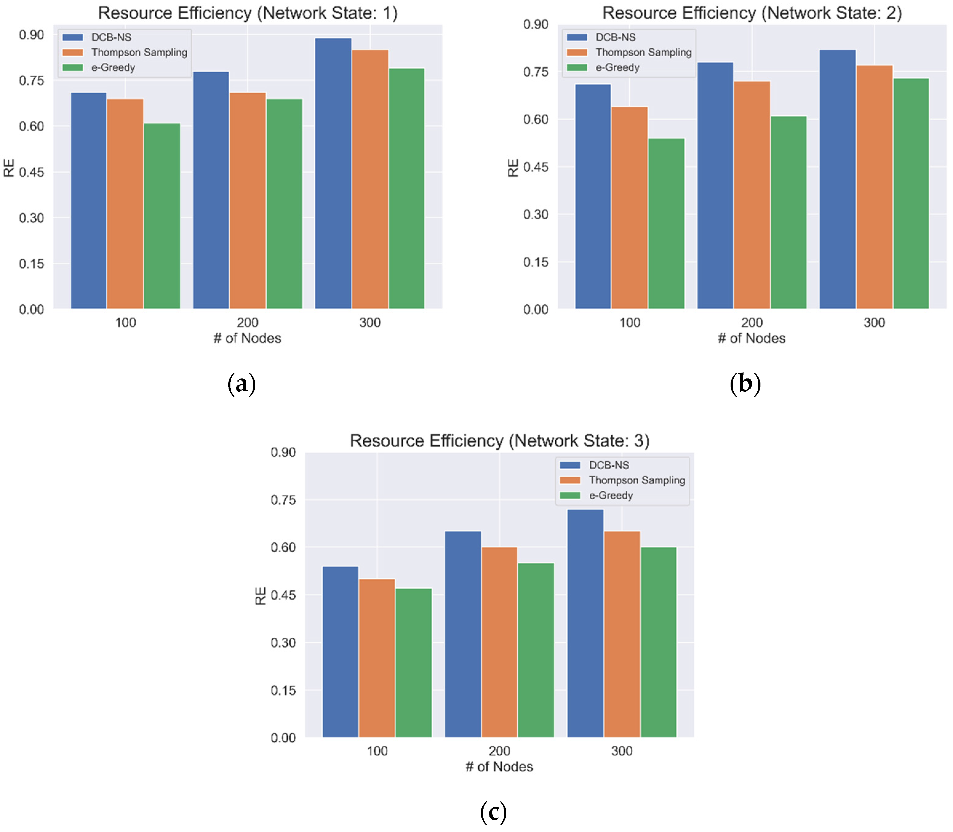
The network RE based on the current network state is also considered, as shown in Figure 5. For this simulation, the average REs for network states 1, 2, and 3, are taken as shown in Figure 4a–c. The results indicate that the proposed scheme can achieve higher RE regardless of the different states of the network. Moreover, the proposed scheme achieves favorable results compared to the other algorithms for all network states and the maximum number of network nodes.

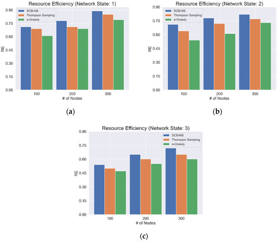
Figure 5. Average Network Resource Efficiency for (a) Network State 1, (b) Network State 2, and (c) Network State 3.

5.3. Network Throughput

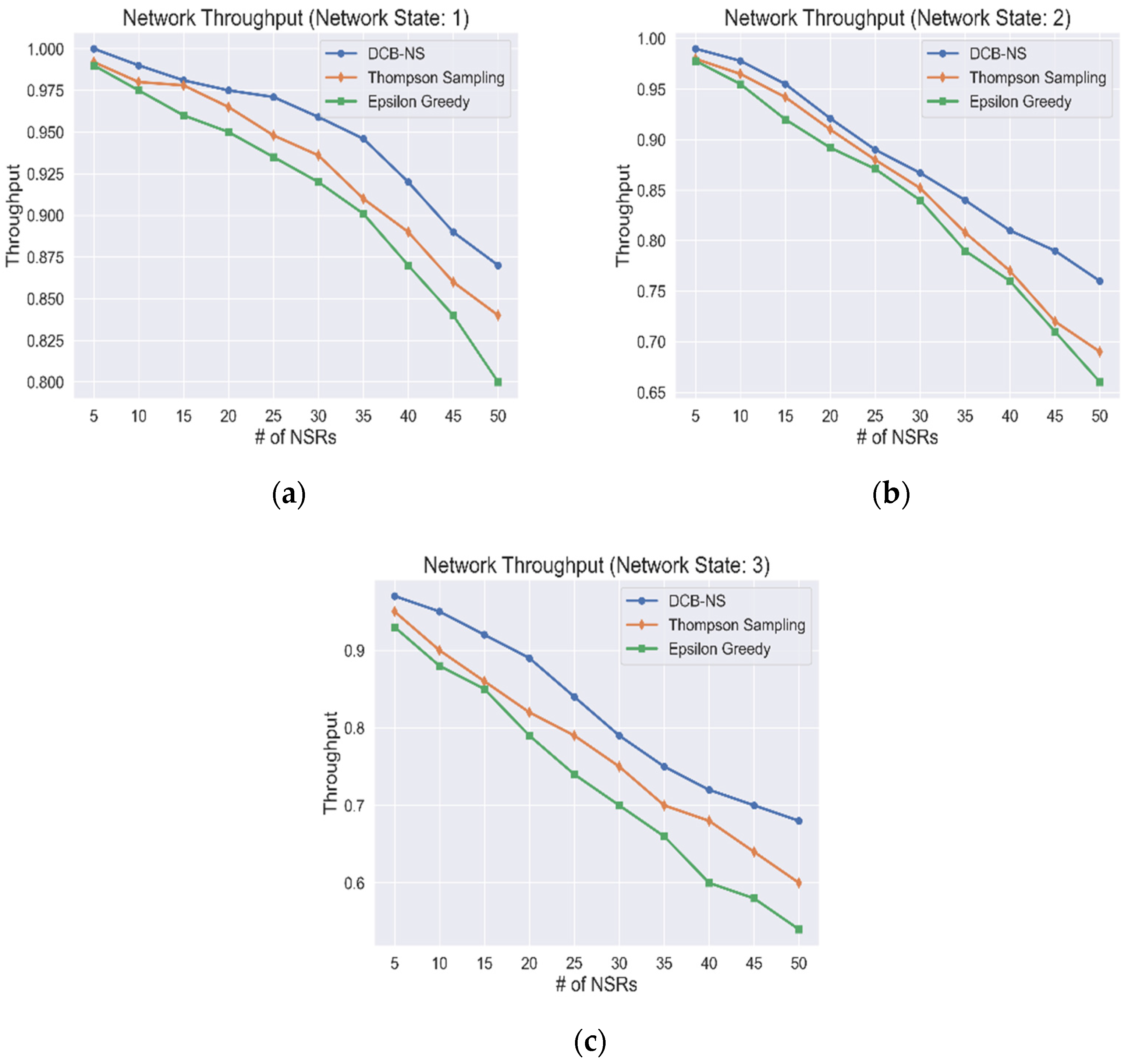
The network throughput for all network states is shown in Figure 6. The simulation results show how the provisioning of network slices is affected by the number of NSRs received in the network. It can be observed that, although the number of provisioned requests has decreased due to the influx of NSRs, the proposed DCB-NS scheme is still able to outperform the other two algorithms used for testing. The proposed scheme can allocate network resources efficiently by implementing node selection and mapping methods. The NVA and maximum data flow computation allow the NSA to select the ideal candidates for network slice creation and deployment. In addition, the goal of the NSA is to maximize its cumulative gain by considering the total resource utilization through the calculation of RIF values. This advantage, in turn, enables the optimal distribution of resources for all NSRs, considering the current network state, thus minimizing the number of unserved requests.

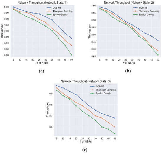
Figure 6. Network Throughput values based on (a) Network State 1, (b) Network State 2, and (c) Network State 3.

Finally, a summary showing an average comparison of the proposed scheme’s performance is provided in Table 4.

Table 4. The proposed scheme’s average performance comparison with the Epsilon–Greedy and Thompson Sampling algorithms.

Algorithm	Rewards	RE	Throughput
DCB-NS	90%	77%	85%
Thompson Sampling	86%	63%	83%
Epsilon-Greedy	77%	60%	80%

6. Conclusions

This paper presents a Deep Contextual Bandits-based network slicing scheme (DCB-NS) that aims to allocate network resources in a 5G network effectively. The proposed scheme uses network theory methods to implement node selection, ranking, and mapping for network slice candidate selection. A Deep RL approach was used to develop a NSA that solves a Contextual Bandit problem. The goal of this agent is to maximize action rewards by selecting and implementing the best possible network slice for each NSR sent to the network. Reward Influencing Factors (RIFs) for the reward calculation were formulated by considering the current network resource utilization. In addition, the Upper Confidence Bound strategy was implemented to balance exploration and exploitation of agent actions for efficient network slice selection.

The simulations showed that the proposed DCB-NS scheme could achieve significantly higher rewards, RE, and network throughput than the Epsilon–Greedy and Thompson sampling methods. With the simulation results, it was observed that the proposed scheme was able to maintain higher performance regardless of the gradual decrease in resource availability with the increasing number of NSRs. The implementation of optimization methods is planned for the future to improve network resource allocation. Dynamic slicing will also be investigated to improve network throughput and RE. Finally, further studies on other RL methods to improve the decision-making capability of the NSA will be conducted.

References

- Henry, S.; Alsohaily, A.; Sousa, E.S. 5G is Real: Evaluating the Compliance of the 3GPP 5G New Radio System with the ITU IMT-2020 Requirements. IEEE Access 2020, 8, 42828–42840. [Google Scholar] [CrossRef]
- Jain, A.; Lopez-Aguilera, E.; Demirkol, I. User association and resource allocation in 5G (AURA-5G): A joint optimization framework. Comput. Netw. 2021, 192, 108063. [Google Scholar] [CrossRef]
- Fantacci, R.; Picano, B. When Network Slicing Meets Prospect Theory: A Service Provider Revenue Maximization Framework. IEEE Trans. Veh. Technol. 2020, 69, 3179–3189. [Google Scholar] [CrossRef]
- Tadros, C.N.; Rizk, M.R.M.; Mokhtar, B.M. Software Defined Network-Based Management for Enhanced 5G Network Services. IEEE Access 2020, 8, 53997–54008. [Google Scholar] [CrossRef]
- Mei, C.; Liu, J.; Li, J.; Zhang, L.; Shao, M. 5G network slices embedding with sharable virtual network functions. J. Commun. Netw. 2020, 22, 415–427. [Google Scholar] [CrossRef]
- Papageorgiou, A.; Fernández-Fernández, A.; Siddiqui, S.; Carrozzo, G. On 5G network slice modelling: Service, resource, or deployment-driven? Comput. Commun. 2020, 149, 232–240. [Google Scholar] [CrossRef]
- Subedi, P.; Alsadoon, A.; Prasad, P.W.C.; Rehman, S.; Giweli, N.; Imran, M.; Arif, S. Network slicing: A next generation 5G perspective. EURASIP J. Wirel. Commun. Netw. 2021, 2021, 1–26. [Google Scholar] [CrossRef]
- Kourtis, M.-A.; Sarlas, T.; Xilouris, G.; Batistatos, M.C.; Zarakovitis, C.C.; Chochliouros, I.P.; Koumaras, H. Conceptual Evaluation of a 5G Network Slicing Technique for Emergency Communications and Preliminary Estimate of Energy Trade-off. Energies 2021, 14, 6876. [Google Scholar] [CrossRef]
- Chagdali, A.; Elayoubi, S.; Masucci, A. Slice Function Placement Impact on the Performance of URLLC with Multi-Connectivity. Computers 2021, 10, 67. [Google Scholar] [CrossRef]
- Alotaibi, D. Survey on Network Slice Isolation in 5G Networks: Fundamental Challenges. Procedia Comput. Sci. 2021, 182, 38–45. [Google Scholar] [CrossRef]
- Sohaib, R.; Onireti, O.; Sambo, Y.; Imran, M. Network Slicing for Beyond 5G Systems: An Overview of the Smart Port Use Case. Electronics 2021, 10, 1090. [Google Scholar] [CrossRef]
- Ojijo, M.O.; Falowo, O.E. A Survey on Slice Admission Control Strategies and Optimization Schemes in 5G Network. IEEE Access 2020, 8, 14977–14990. [Google Scholar] [CrossRef]
- Ye, Q.; Li, J.; Qu, K.; Zhuang, W.; Shen, X.S.; Li, X. End-to-End Quality of Service in 5G Networks: Examining the Effectiveness of a Network Slicing Framework. IEEE Veh. Technol. Mag. 2018, 13, 65–74. [Google Scholar] [CrossRef]
- Thantharate, A.; Paropkari, R.; Walunj, V.; Beard, C. DeepSlice: A Deep Learning Approach towards an Efficient and Reliable Network Slicing in 5G Networks. In Proceedings of the 2019 IEEE 10th Annual Ubiquitous Computing, Electronics and Mobile Communication Conference, UEMCON 2019, New York, NY, USA, 10–12 October 2019; pp. 762–767. [Google Scholar] [CrossRef]
- Thantharate, A.; Paropkari, R.; Walunj, V.; Beard, C.; Kankariya, P. Secure5G: A Deep Learning Framework Towards a Secure Network Slicing in 5G and Beyond. In Proceedings of the 2020 10th Annual Computing and Communication Workshop and Conference, CCWC 2020, Las Vegas, NV, USA, 6–8 January 2020; pp. 852–857. [Google Scholar] [CrossRef]
- Abbas, K.; Afaq, M.; Khan, T.A.; Mehmood, A.; Song, W.-C. IBNSlicing: Intent-Based Network Slicing Framework for 5G Networks using Deep Learning. In Proceedings of the APNOMS 2020–2020 21st Asia-Pacific Network Operations and Management Symposium: Towards Service and Networking Intelligence for Humanity, Daegu, Korea, 22–25 September 2020; pp. 19–24. [Google Scholar] [CrossRef]
- Sharma, N.; Kumar, K. Resource allocation trends for ultra-dense networks in 5G and beyond networks: A classification and comprehensive survey. Phys. Commun. 2021, 48, 101415. [Google Scholar] [CrossRef]
- Ejaz, W.; Sharma, S.K.; Saadat, S.; Naeem, M.; Anpalagan, A.; Chughtai, N. A comprehensive survey on resource allocation for CRAN in 5G and beyond networks. J. Netw. Comput. Appl. 2020, 160, 102638. [Google Scholar] [CrossRef]
- Pereira, R.; Lieira, D.; Silva, M.; Pimenta, A.; Da Costa, J.; Rosário, D.; Villas, L.; Meneguette, R. RELIABLE: Resource Allocation Mechanism for 5G Network using Mobile Edge Computing. Sensors 2020, 20, 5449. [Google Scholar] [CrossRef]
- Guan, W.; Wen, X.; Wang, L.; Lu, Z.; Shen, Y. A service-oriented deployment policy of end-to-end network slicing based on complex network theory. IEEE Access 2018, 6, 19691–19701. [Google Scholar] [CrossRef]
- Sciancalepore, V.; Zanzi, L.; Costa-Perez, X.; Capone, A. ONETS: Online Network Slice Broker From Theory to Practice. IEEE Trans. Wirel. Commun. 2022, 21, 121–134. [Google Scholar] [CrossRef]
- Abidi, M.H.; Alkhalefah, H.; Moiduddin, K.; Alazab, M.; Mohammed, M.K.; Ameen, W.; Gadekallu, T.R. Optimal 5G network slicing using machine learning and deep learning concepts. Comput. Stand. Interfaces 2021, 76, 103518. [Google Scholar] [CrossRef]
- Li, X.; Guo, C.; Gupta, L.; Jain, R. Efficient and Secure 5G Core Network Slice Provisioning Based on VIKOR Approach. IEEE Access 2019, 7, 150517–150529. [Google Scholar] [CrossRef]
- Fossati, F.; Moretti, S.; Perny, P.; Secci, S. Multi-Resource Allocation for Network Slicing. IEEE/ACM Trans. Netw. 2020, 28, 1311–1324. [Google Scholar] [CrossRef]
- Sun, Y.; Qin, S.; Feng, G.; Zhang, L.; Imran, M.A. Service Provisioning Framework for RAN Slicing: User Admissibility, Slice Association and Bandwidth Allocation. IEEE Trans. Mob. Comput. 2021, 20, 3409–3422. [Google Scholar] [CrossRef]
- Li, T.; Zhu, X.; Liu, X. An End-to-End Network Slicing Algorithm Based on Deep Q-Learning for 5G Network. IEEE Access 2020, 8, 122229–122240. [Google Scholar] [CrossRef]
- Jungnickel, D. Graphs, Networks, and Algorithms, 2nd ed.; Springer: New York, NY, USA, 2005. [Google Scholar]
- Li, X.; Guo, C.; Xu, J.; Gupta, L.; Jain, R. Towards Efficiently Provisioning 5G Core Network Slice Based on Resource and Topology Attributes. Appl. Sci. 2019, 9, 4361. [Google Scholar] [CrossRef] [Green Version]
- Van Steen, M. Graph Theory and Complex Networks: An Introduction; University of Twente: Enschede, The Netherlands, 2010. [Google Scholar]
- Slivkins, A. Introduction to Multi-Armed Bandits. arXiv 2019, arXiv:1904.07272. Available online: http://arxiv.org/abs/1904.07272 (accessed on 3 March 2022).
- Sutton, R.S.; Barto, A.G. Reinforcement Learning: An Introduction, 2nd ed.; The MIT Press: Cambridge, MA, USA, 2017. [Google Scholar]
- Singh, A. Reinforcement Learning Based Empirical Comparison of UCB, Epsilon-Greedy, and Thompson Sampling. Int. J. Aquat. Sci. 2021, 12, 1–9. Available online: http://www.journal-aquaticscience.com/article_134653_449d479986f2096f94b09b7227ae8a2d.pdf (accessed on 24 March 2022).
Publisher’s Note: MDPI stays neutral with regard to jurisdictional claims in published maps and institutional affiliations. |
© 2022 by the authors. Licensee MDPI, Basel, Switzerland. This article is an open access article distributed under the terms and conditions of the Creative Commons Attribution (CC BY) license (https://creativecommons.org/licenses/by/4.0/).