


Abstract
We introduce a deterministic class of constraint-coupled reaction–diffusion systems in which an internally generated field modulates transport and reaction processes while being regenerated by the same dynamics that it regulates. This feedback structure provides a minimal mathematical framework for studying dynamically consequential endogenous regulation in spatially extended non-equilibrium systems; the presence of a causal loop alone is not identified with organizational autonomy. The model is formulated as a quasilinear parabolic system on a bounded domain. Positivity, boundedness, viability, equilibrium stability, and spatial localization are treated as distinct mathematical properties. Under structural assumptions on the diffusion and reaction terms, we establish local classical well-posedness, preservation of non-negativity, and global existence under boundedness or forward-invariant-region conditions. Viability is formulated as forward invariance of subsets of an infinite-dimensional phase space rather than as a local pointwise balance. A minimal three-field realization, consisting of a resource field, an organizing field, and a constraint field, is then analyzed. We derive conditions for the existence of positive homogeneous equilibria, obtain sufficient criteria for homogeneous and full modal stability, and characterize stationary and oscillatory spatial instability thresholds through a mode-dependent dispersion relation. We complement the analysis with conservative two-dimensional finite-volume simulations. Below the predicted spatial-instability threshold, perturbations decay, whereas above threshold a persistent heterogeneous state forms with a dominant scale consistent with the dispersion relation. Constraint level sets, occupied fraction, connected components, and concentration indices quantify the resulting dynamically generated localization. Feedback-ablation controls show that, for the representative parameter set, removing either transport or reaction feedback eliminates the finite-wavenumber instability, while alternative bounded monotone constitutive laws preserve spatial patterning. The framework therefore distinguishes externally imposed regulation, passive outputs, and dynamically consequential endogenous feedback, and provides a basis for investigating bounded self-maintenance and localization without equating loop topology with autonomy.
1. Introduction
1.1. Reaction–Diffusion Organization and the Present Problem
The emergence and persistence of organized spatial structures in non-equilibrium systems is a central problem in nonlinear dynamics. Reaction–diffusion equations provide one of the classical mathematical frameworks in which spatial organization can arise from the interaction of local kinetics and transport. Turing’s analysis showed that diffusion can destabilize an otherwise stable homogeneous chemical state and thereby generate a characteristic spatial pattern [1]. Since then, reaction–diffusion theory has been extended to stationary patterns, traveling fronts, oscillatory structures, wave instabilities, localized states, and transitions between different spatiotemporal regimes [2,3,4].
The classical framework usually assumes that the principal elements regulating the dynamics are specified in advance. Diffusion coefficients, reaction pathways, coupling strengths, external resource terms, and boundary conditions are prescribed as fixed components of the model. The resulting system may generate highly complex behavior, but the effective operators governing that behavior are not normally produced by the evolving state itself.
The present work investigates a different situation. We consider reaction–diffusion systems coupled to an additional field that is generated by the internal dynamics and that modifies the subsequent transport and reaction processes of the variables contributing to its production. We refer to this field as a constraint field. Its defining property is not simply that it is an additional chemical or biological variable, but that it occupies a particular functional position within the coupled dynamics.
At a schematic level, the relevant feedback architecture is
where
denotes the collection of primary fields, C is the constraint field, and denotes the state-dependent operator acting on the primary variables. The first arrow expresses the production or regeneration of C by the internal state. The second expresses the dependence of transport or reaction processes on C. The final arrow closes the feedback loop by allowing this regulation to alter the future evolution of the variables that maintain the constraint.
The mathematical problem is therefore not only to determine whether the system forms a pattern. It is also to determine whether the internally generated regulatory field remains dynamically active, whether it contributes to maintaining the system inside an admissible region, and whether it can support persistent spatially localized regimes.
1.2. Internally Generated Constraints and Endogenous Regulation
The term autonomous has a standard meaning in dynamical-systems theory: an evolution equation is autonomous when its governing law has no explicit dependence on time. That usage is distinct from the organizational interpretation discussed in the literature on closure of constraints.
In the present paper we do not infer organizational autonomy from the existence of a causal loop alone. We use the more specific term endogenous regulation for the mathematical property that part of the effective regulatory structure is generated by the evolving state and acts back on that state. The equations themselves remain fixed; what changes during the evolution is the effective operator experienced by the primary variables because coefficients or reaction rates depend on a dynamically produced field. Whether this feedback is dynamically consequential is a comparative question tested against feedback-ablated controls in Section 8. Organizational autonomy, when discussed below, is therefore a broader interpretation requiring additional persistence and viability criteria.
For example, an operator of the form
contains both transport and reaction mechanisms whose effective form depends on C. If C is itself produced by the fields , then the system contributes to the construction of the regulatory conditions under which it subsequently evolves.
This idea is related to several established traditions, although the present paper does not attempt to identify them as mathematically equivalent. The theory of dissipative structures emphasizes that organized states can be sustained far from equilibrium through continuous energetic or material throughput [5]. The theory of adaptive and coevolutionary systems studies situations in which the state of a system modifies the structure governing its future interactions [6]. Theories of biological autonomy and closure of constraints emphasize networks in which regulatory or constraining processes depend on one another for their continued maintenance [7,8].
The present contribution is narrower and more explicitly mathematical. It does not propose a general theory of biological autonomy. Instead, it formulates a class of deterministic partial differential equations in which internally generated regulation can be studied using the methods of quasilinear parabolic equations, invariant-region theory, linear stability, bifurcation analysis, and numerical continuation.
The distinction between an internally generated constraint, a passive output, and an externally imposed control field is essential. A field produced by the system but having no feedback action is merely an output. A field that modifies the dynamics but is fixed externally is a control parameter or imposed environment. A dynamically generated constraint must perform both functions: it must be produced internally and must influence processes relevant to its own continued production.
This functional definition does not require C to represent a literal physical boundary. Depending on the application, it may represent a structural matrix, a permeability field, an effective mobility, an inhibitory environment, a regulatory concentration, or another coarse-grained quantity that modifies the available dynamical pathways.
1.3. Relation to State-Dependent Transport and Cross-Diffusion
The general class studied below has the form
on a bounded spatial domain. Here denotes a prescribed environmental or resource field, H describes production and degradation of the constraint, and the functions and describe its action on transport and local kinetics.
Because the diffusion coefficients depend on an evolving state variable, the system belongs to the broad class of quasilinear reaction–diffusion equations. It is also related to density-dependent transport and cross-diffusion models, in which the movement of one component depends on the local concentration of another [9,10]. The emphasis here is, however, different. The variable C is interpreted through the feedback role expressed in (1), rather than only as another interacting population or chemical species.
State-dependent transport can contribute to retention and concentration. For instance, if , a region with elevated C reduces the mobility of . Such retention may sharpen, stabilize, or prolong an existing spatial structure. Nevertheless, reduced mobility alone does not guarantee the formation of a pattern.
Indeed, consider a spatially homogeneous equilibrium . Since
the linearization of the transport term satisfies
The derivative does not generate a linear cross-diffusion term about a constant equilibrium because it multiplies the equilibrium gradient, which vanishes. Consequently, a spatial instability depends on the complete reaction–transport coupling, not merely on the fact that the constraint reduces diffusion.
This observation motivates the inclusion of both transport regulation and reaction feedback in the minimal model developed later. Constraint-mediated retention may influence nonlinear localization, while constraint-dependent reaction terms can enter the Jacobian directly and therefore affect the onset of a linear instability.
The present parabolic formulation also belongs to a wider landscape of non-equilibrium transport models. Hyperbolic advection–diffusion theories replace the infinite propagation speed of classical Fourier–Fick transport by finite-speed relaxation mechanisms and require correspondingly different analytical and numerical tools [11]. Generalized heat-conduction models derived from the Boltzmann transport equation extend this viewpoint to moving media while enforcing Galilean invariance [12]. Recent work on thermal-wave reflection and refraction in heterogeneous two-layer composites further illustrates how state-dependent or spatially heterogeneous transport, interfaces, and moving sources can produce localized energy accumulation and nonclassical propagation [13]. These models are not mathematically identical to the reaction–diffusion system studied here, but they place constraint-dependent diffusivity within the broader context of generalized transport in heterogeneous non-equilibrium media.
The present construction also overlaps with several more direct traditions that must be kept conceptually separate. In Keller–Segel chemotaxis, aggregation is driven by a cross-gradient flux, typically of the form , whereas the minimal model below uses a diagonal flux : the field c changes the magnitude of ordinary diffusion but does not generate directed drift [14]. Classical cross-diffusion systems likewise allow one component’s flux to depend directly on gradients of other components [9,10]. Models of protocell self-maintenance may instead couple reaction–diffusion processes to an explicit moving membrane or free boundary [15,16]. Localized states in reaction–diffusion systems can arise through subcritical Turing bifurcations, wave pinning, front interactions, and homoclinic snaking [17,18,19]. The present work does not claim that localization itself is a new mechanism. Its narrower question is how a field generated by the active state can modulate both transport and kinetics, how this modulation can be placed inside a viability framework, and whether its dynamical contribution survives explicit feedback-removal controls.
A related earlier preprint by one of the present authors proposed the broader “Constraint Emergence Hypothesis” in the context of origins-of-life scenarios [20]. That work is conceptual in scope and discusses constraint fields, organizational closure, and proto-individuality. The present article is deliberately narrower and should not be read as a second presentation of the same result. Here the focus is a specified uniformly parabolic PDE class, with explicit hypotheses for well-posedness and invariant regions, a minimal three-field realization, modal stability and bifurcation criteria, reproducible two-dimensional finite-volume simulations, and ablation tests of the feedback mechanism. No numerical dataset from the earlier preprint is reused here; all computations reported below were generated specifically for the present model and are reproducible from the accompanying code.
1.4. Viability, Stability, and Self-Maintenance
A central concept of the paper is viability. Informally, a system is viable when its trajectory remains inside a prescribed set of physically and organizationally admissible configurations.
In a reaction–diffusion problem, the state at a given time is not a point of , but a spatial profile. Viability must therefore be formulated in an infinite-dimensional phase space such as
A subset is forward invariant when
This formulation is closely related to viability theory [21]. For reaction–diffusion systems, positively invariant regions can often be obtained from inward-pointing conditions on the reaction vector field, together with a diffusion structure compatible with the maximum principle [22,23].
The use of forward invariance corrects a common ambiguity. Conditions such as
describe a desired range, but they do not show that the PDE preserves that range. A viability theorem must examine the vector field on every relevant boundary face and prove that the trajectory cannot exit.
It is also necessary to distinguish positivity from persistence. A constraint field may satisfy
while becoming arbitrarily small and dynamically ineffective. A quantitatively maintained constraint requires either a positive lower bound or persistence above an operational threshold on a nonempty spatial region.
Viability must also be separated from equilibrium stability. A forward-invariant region can contain stable or unstable equilibria, periodic trajectories, spatially patterned states, or more complicated bounded dynamics. Stability concerns the response of a particular trajectory or invariant set to perturbations. Viability concerns continued membership in an admissible region.
Similarly, a forward-invariant set is not automatically an attractor. The existence of a global attractor for a dissipative PDE normally requires a global semiflow, a bounded absorbing set, and an appropriate compactness or asymptotic compactness property [24,25,26]. The present paper therefore uses the term viability region for the invariant sets established below and reserves the term attractor for situations in which an attraction property has been proved.
1.5. Dynamically Generated Localization
If the constraint field becomes spatially heterogeneous, its level sets define regions in which transport and reaction dynamics differ from those of the surrounding medium. Given an operational threshold , define
The set is called a constraint-defined domain. Its boundary is not prescribed as part of the geometry of the problem. It is generated by the evolving solution.
This interpretation connects the model to the broader mathematical theory of localized states, in which spatially confined structures can arise through instability, bistability, front interactions, or pinning mechanisms [17]. In the present setting, however, localization is measured through the dynamically generated constraint field rather than by assuming a material enclosure in advance.
The threshold is an operational parameter. Different threshold values may produce different geometries, and the connectedness of must therefore be studied over a nontrivial range of thresholds. The set should not be interpreted as an independent physical object added to the equations. It is a diagnostic derived from the field C.
When C is sufficiently regular and
the normal velocity of the level-set boundary is
This identity shows that expansion or contraction cannot be inferred from the local production term alone. Constraint production, degradation, diffusion, and the local curvature of the profile all contribute to the motion of the threshold boundary.
Likewise, an increase in the number of connected components of requires the creation of new extrema or the deformation of the field through a critical threshold. Such behavior cannot be deduced from the feedback diagram alone. It must be established through bifurcation analysis, nonlinear continuation, or direct numerical integration.
For the same reason, a loss of connectedness of will be described as level-set splitting. It will not be identified with reproduction unless the resulting components are shown to persist independently and to retain the internal feedback required for their own viability.
1.6. Objectives and Organization of the Paper
The objective of this work is to provide a mathematically controlled framework for autonomous constraint-coupled reaction–diffusion systems. The analysis begins by defining a deterministic quasilinear parabolic class with explicit spatial domain, boundary conditions, phase space, regularity assumptions, and notion of solution.
The first analytical task is to establish that the system generates a well-defined evolution. Local existence and uniqueness are obtained under uniform parabolicity and regularity assumptions, while quasi-positivity is used to preserve the non-negative state space. Global existence is then derived from a continuation criterion together with dissipative estimates or bounded invariant regions.
The second task is to formulate viability rigorously. Rather than treating pointwise bounds as assumed properties, the paper derives inward-pointing conditions under which the associated phase-space rectangle is forward invariant. This yields sufficient conditions for boundedness, persistence, and maintenance of a positive constraint threshold.
The third task is to introduce a minimal three-field model consisting of a resource field, an organizing field, and a constraint field. The organizing field produces the constraint, while the constraint modifies both its mobility and its local production. The model is constructed so that positivity and boundedness can be established explicitly.
The fourth task is to analyze the homogeneous equilibria and their stability. Positive equilibria are reduced to a scalar equation, and sufficient conditions for existence, uniqueness, and local stability are derived. Spatial perturbations are then studied through the dispersion relation
where is the reaction Jacobian, is the diffusion matrix at the equilibrium, and q is a Laplacian eigenvalue.
The final task is computational. Numerical continuation and direct simulation are used to test whether the analytical instability conditions lead to persistent nonlinear patterns or localized constraint-defined domains. Particular attention is given to the size, connectedness, and time evolution of the threshold set (7), together with feedback-ablation controls and constitutive-law sensitivity tests. These computations test the mathematical mechanisms developed in the paper and delimit the claims to the representative parameter regimes actually studied.
Section 2 introduces the general deterministic constraint-coupled system. Section 3 establishes well-posedness, positivity, continuation criteria, and global existence. Section 4 develops the invariant-region formulation of viability. Section 5 introduces the minimal three-field model, and Section 6 analyzes its homogeneous equilibria and sufficient stability conditions. Section 7 derives the spatial dispersion relation and the associated bifurcation conditions. Section 8 presents the continuation, direct simulations, feedback-ablation controls, constitutive-law sensitivity tests, and level-set diagnostics. Section 9 discusses interpretation, limitations, and stochastic extensions, and Section 10 summarizes the principal conclusions.
2. Deterministic Constraint-Coupled Reaction–Diffusion Systems
We now formulate the deterministic class of spatially extended systems studied throughout the paper. The objective is to define a well-posed quasilinear parabolic initial-boundary value problem and, within that mathematical class, to identify the structural conditions that distinguish a dynamically generated constraint from an ordinary interacting field.
The formulation is intentionally general. It is not tied to a particular chemical mechanism, biological process, or engineering realization. Instead, it describes systems in which an evolving field is produced by the internal state and subsequently modifies the transport or reaction processes of the variables involved in its production. The resulting PDE belongs to the broad theory of quasilinear parabolic systems [27,28], while its state-dependent transport structure is related to density-dependent diffusion and cross-diffusion models [9,10].
2.1. Spatial Domain, Fields, and Environmental Input
Let
be a bounded and connected domain whose boundary is of class . The outward unit normal to the boundary is denoted by n.
The system contains N primary scalar fields
and one scalar constraint field
where and . We write
for the primary and complete state vectors, respectively.
The variables may represent concentrations, densities, activities, populations, or other non-negative spatially distributed quantities. The interpretation of C is not determined solely by its physical units. It is determined by its position in the feedback structure: the field must be internally generated and must modify processes that affect the future evolution of the primary variables.
The dynamics may also depend on a prescribed environmental field
This field may represent an externally supplied resource, an energetic input, a chemical potential, or another environmental condition. Unlike x and C, the field is not included among the evolving state variables in the present analysis. It acts as a prescribed input to the reaction terms.
2.2. General Evolution Equations
The deterministic constraint-coupled system is
The coefficient is the effective diffusivity of the i-th primary field, while is the diffusivity of the constraint. The function contains the local production, consumption, conversion, decay, and environmental coupling terms for . The function H describes the local production and degradation of C.
A useful representation of the constraint source is
where is a production coefficient, is a decay coefficient, and F measures the contribution of the internal state and environment to constraint production. This decomposition is not required for the entire general theory, but it is useful when discussing persistence and upper bounds.
In compact notation, the system may be written as
where
and
Because the coefficients depend on an evolving component of the state, the system is quasilinear rather than semilinear. Standard local existence theory therefore requires regularity of the coefficient maps, uniform ellipticity, and suitable compatibility conditions [27,28].
2.3. Initial and Boundary Conditions
We impose homogeneous no-flux boundary conditions,
together with the initial conditions
The no-flux conditions isolate the internal redistribution and reaction dynamics from direct material exchange through . They do not imply energetic or environmental closure, because the prescribed field may supply or remove resources through and H.
Dirichlet, Robin, or nonlinear exchange conditions could be introduced to represent contact with an external reservoir. Such choices would modify the mass balances, maximum-principle arguments, and invariant-region conditions. They are therefore excluded from the main analytical development.
2.4. Phase Space and Admissible States
The state of a reaction–diffusion system is a spatial profile rather than a point of . We therefore take
as the phase space, equipped with the norm
Its non-negative cone is
The use of makes positivity, upper and lower thresholds, and invariant rectangles unambiguous at every spatial point. Weak-solution theories may instead be developed in Sobolev or Lebesgue spaces, but the pointwise formulation is more convenient for the viability analysis undertaken here.
Let
be a bounded pointwise rectangle. It induces the phase-space set
It is , rather than the finite-dimensional rectangle by itself, that may be forward invariant under the PDE semiflow. Positively invariant rectangles for nonlinear diffusion systems are classically obtained through maximum-principle and inward-pointing arguments [22,23].
2.5. Structural Assumptions
We now state the hypotheses used in the well-posedness, positivity, and viability analysis.
Assumption 1
(Uniform ellipticity). For every , the map
belongs to , and there exist constants such that
for every . In addition, .
Uniform ellipticity ensures that all transport equations remain genuinely parabolic. If one of the diffusivities were permitted to vanish, the problem would become degenerate and would require a different existence theory.
Assumption 2
(Local regularity of the nonlinearities). For every bounded interval of admissible environmental values, the functions
and
are continuous in all variables and locally Lipschitz continuous with respect to , uniformly on bounded sets of Φ.
This hypothesis includes polynomial, rational, saturating, and Hill-type kinetics on bounded subsets of the state space. Its principal analytical role is to provide local uniqueness and continuous dependence on initial data.
Assumption 3
(Admissible environmental field). The environmental field satisfies
and there exist constants such that
for every and .
The boundedness of prevents the prescribed environment from introducing an uncontrolled singular forcing. The lower bound need not be positive in the general theory, although particular persistence results may require a strictly positive resource level.
Assumption 4
(Quasi-positivity). For every non-negative state , every admissible value of Φ, and every ,
and
Quasi-positivity means that the local reaction vector field cannot point outward through a boundary face of the non-negative orthant. It does not require every source term to be positive. Consumption, decay, and competition remain admissible away from the corresponding zero boundary. Together with the maximum principle, this condition is the standard mechanism by which non-negativity is preserved in reaction–diffusion systems [23,29].
Assumption 5
(Initial data). The initial state satisfies
For classical solutions, the initial data are assumed to possess the additional spatial regularity and boundary compatibility introduced in Assumption 6 and (59).
2.6. Classical and Maximal Solutions
Definition 1
Definition 2
(Maximal solution). A classical solution is maximal if it is defined on an interval , where , and cannot be extended as a classical solution beyond .
The continuation result established in Section 3 will show that a finite maximal time can occur only if the solution becomes unbounded or leaves a region in which the coefficients remain regular. This is consistent with standard continuation principles for quasilinear parabolic systems [27,30].
2.7. Definition and Action of a Dynamically Generated Constraint
From the formal PDE viewpoint, C is one component of the state vector. It evolves, diffuses, and participates in nonlinear interactions. Its special status is therefore functional rather than algebraic.
Definition 3
(Dynamically generated constraint field). The field C is called a dynamically generated constraint field when its production depends nontrivially on the internal state,
and when it acts back on at least one primary equation. The feedback condition holds when, for some i,
or
The generation condition excludes a field whose evolution is independent of the internal state. The feedback condition excludes a passive by-product that records activity without affecting it. Together, they define the minimal loop
The interpretation is relational. A substance or field acts as a constraint only because of the causal role it plays in the coupled dynamics.
The constraint may regulate transport. A typical bounded decreasing diffusivity is
where
This expression reduces mobility as C increases while preserving the uniform bounds
The positive lower bound is analytically significant. The simpler law
approaches zero as and therefore fails to satisfy the global ellipticity assumption unless an independent upper bound for C has already been established.
The constraint may also regulate local kinetics. A representative form is
where
is a bounded saturating response. Such bounded feedback laws are preferable to unrestricted linear amplification when global a priori bounds are sought.
Environmental coupling may itself depend on the constraint. For example,
allows C to alter the efficiency with which an externally supplied resource is captured, transformed, or retained.
Transport regulation, reaction regulation, and environmental coupling are not interchangeable. The first modifies spatial redistribution, the second changes local production or loss, and the third changes the relation between the internal state and the prescribed environment. A particular model may contain one or several of these mechanisms.
2.8. External Driving and Endogenous Regulation
The presence of does not contradict the organizational meaning of autonomy used in this work. A non-equilibrium system may require continuous external supply while regulating internally how that supply is used, as is typical of dissipative systems [5].
External driving supplies material, energy, or another resource. External control prescribes the regulatory structure that determines how the system evolves. Internal constraint generation occurs when the evolving state produces the field that performs part of this regulatory role. These situations are mathematically and conceptually distinct.
The systems considered here may therefore be externally driven without being externally controlled at the level of C. The field provides conditions under which activity can persist, whereas the constraint field contributes endogenously to the spatial and dynamical organization of that activity. Autonomy in this restricted sense does not mean energetic independence from the environment.
2.9. Mass Balances and Homogeneous States
Integrating the primary equations over and using the no-flux boundary conditions gives
Similarly,
State-dependent diffusion redistributes the fields within the domain but does not directly alter their total mass under no-flux boundary conditions. Changes in total mass arise from the local source terms. Consequently, reduced diffusivity may increase local retention, but it cannot create constraint mass. Persistent localization must result from the interaction between redistribution and local production or loss.
If is spatially homogeneous, a spatially homogeneous state has the form
and satisfies
A homogeneous equilibrium
therefore satisfies
The equality expresses a balance between production and loss of the constraint. It does not establish stability, viability, or localization. These properties must be analyzed separately.
Spatial heterogeneity may arise from heterogeneous initial data, heterogeneous environmental forcing, nonlinear front dynamics, or instability of a homogeneous equilibrium. The analysis below concentrates on the last mechanism, while retaining bistability and finite-amplitude localization as distinct possibilities.
2.10. Deterministic Scope and Stochastic Extensions
The principal analytical problem is deterministic. This choice separates the structural consequences of internally generated feedback from the additional regularity, positivity, and interpretation problems introduced by stochastic forcing.
A formal additive space–time white-noise term in the constraint equation would generally be incompatible with pointwise non-negativity. Moreover, in dimensions , the associated stochastic convolution need not be function-valued, so nonlinear expressions such as and may cease to be classically defined. These issues are standard in the theory of stochastic partial differential equations [31,32].
A more suitable stochastic extension has the abstract form
where has a spatially regular covariance operator and is selected consistently with the desired state space and positivity properties. Such extensions are discussed only in Section 9.
The deterministic initial-boundary value problem studied in the following sections is therefore
Under Assumptions 1–5, this is a uniformly parabolic quasilinear system with locally Lipschitz nonlinearities. Section 3 establishes local existence, uniqueness, preservation of non-negativity, and the continuation criterion. Global existence is then obtained when suitable a priori bounds or bounded forward-invariant regions prevent blow-up [30,33].
3. Well-Posedness, Positivity, and Global Existence
The notions of viability, equilibrium stability, bifurcation, and localization presuppose that the constraint-coupled system generates a mathematically well-defined evolution. We therefore establish local existence, uniqueness, preservation of non-negativity, and a continuation criterion for the initial-boundary value problem (55). The analysis follows the standard theory of uniformly parabolic quasilinear systems, together with maximum-principle and comparison arguments [23,27,28,29].
These tools are classical and are not claimed as new. The novelty sought here is in their organization around a state-generated regulatory field and in the explicit hierarchy of questions to which they are applied: physical admissibility, constraint persistence, organizational viability, homogeneous stability, spatial instability, and nonlinear constraint-defined localization. The invariant-region arguments in Section 4 are likewise applications of the classical Chueh–Conley–Smoller/maximum-principle construction, specialized to the present constraint-coupled class. The contribution is therefore not a new general existence or invariant-region technique, but a mathematically explicit framework and worked model in which endogenous operator modulation can be separated from ordinary reaction–diffusion pattern formation by analytical and numerical controls.
These properties have different meanings. Local well-posedness ensures that an admissible initial profile determines a unique trajectory for a nonzero time interval. Positivity guarantees that concentrations and constraint intensities do not leave the physically relevant state space. Global existence excludes finite-time breakdown. None of these statements, by itself, implies convergence to equilibrium, persistence above a positive constraint threshold, stability of a particular state, or spatial localization.
3.1. Classical Regularity and Local Well-Posedness
The local Lipschitz assumptions introduced in Assumption 2 are sufficient for several mild or weak formulations. To work with pointwise maximum principles and classical invariant-region arguments, we impose stronger Hölder regularity.
Assumption 6
(Classical regularity). Let . For every ,
and the nonlinearities and are locally with respect to , uniformly for Φ in bounded sets. For every finite , the environmental field satisfies
The initial state satisfies
together with the compatibility conditions
These assumptions are convenient rather than conceptually indispensable. Weaker hypotheses can be used in maximal-regularity, , or weak-solution settings. The present choice ensures that the solution is regular enough for the positivity and invariant-region arguments to be performed pointwise.
Theorem 1
(Local classical well-posedness). Suppose that Assumptions 1, 3, 5, and 6 hold. Then, there exists a maximal time
and a unique classical solution
of (55) on . For every ,
The solution depends continuously on the initial data on every compact subinterval of .
Proof.
The principal diffusion matrix is
By Assumption 1, there is a constant
such that
for every and every admissible state. The system is therefore uniformly normally elliptic.
The coefficient maps possess the regularity specified in Assumption 6, and the reaction map is locally Lipschitz in the state variables. The homogeneous Neumann boundary operators satisfy the standard compatibility and complementing conditions. Classical quasilinear parabolic theory therefore gives local existence, uniqueness, regularity, and continuous dependence [27,28].
The solution can be continued uniquely while its range remains inside a bounded region on which the coefficients and nonlinearities retain the required regularity and uniform ellipticity. The supremum of all such existence intervals defines . □
The theorem concerns the existence of a mathematical trajectory. It does not yet show that the solution remains in the non-negative cone. That property follows from the quasi-positivity conditions.
3.2. Preservation of Non-Negativity and Strict Positivity
The non-negative cone defined in (24) is the physically relevant state space. Assumption 4 ensures that, on a boundary face where one component vanishes, its local reaction term cannot force that component to become negative.
Theorem 2
(Preservation of non-negativity). Assume the hypotheses of Theorem 1 and Assumption 4. If
then
Equivalently,
for every , every , and every .
Proof.
We give the argument for . The proof for C is analogous.
Suppose that becomes negative. Since the initial data are non-negative and the solution is continuous, there is a first time and a point at which
and the solution is about to cross into negative values.
If , then has a spatial minimum at , so
At this point,
All other components remain non-negative up to , and quasi-positivity gives
when . Hence
which contradicts a first crossing from non-negative to negative values.
If the minimum is attained on , the homogeneous Neumann condition and the parabolic boundary maximum principle yield the same conclusion. For C, one uses at a first zero minimum and . Thus, no component can leave the non-negative cone. This is the standard invariant-cone argument based on the parabolic maximum principle [23,29]. □
Quasi-positivity does not require every reaction term to be non-negative. A degradation term such as is compatible with the condition because it vanishes when . Likewise, does not threaten positivity because it vanishes at . A term that remained strictly negative when its corresponding component vanished would instead point outward from the non-negative cone.
For the decomposition
constraint quasi-positivity is equivalent to
for every non-negative x and every admissible environmental value.
Non-negativity allows a component to vanish identically. Under the strong maximum principle, nontrivial components become strictly positive at every positive time.
Proposition 1
(Strict positivity of nontrivial components). Assume the hypotheses of Theorem 2 and suppose that Ω is connected. If
then
for every and .
If , or if is strictly positive on a nonempty space–time region, then, under the usual strong maximum-principle hypotheses,
for every and every later positive time.
Proof.
Fix . Since the trajectory is bounded on and is locally Lipschitz, there exists such that, along the solution,
Consequently,
The strong parabolic maximum principle, together with the connectedness of , implies strict positivity for whenever the initial component is non-negative and nontrivial. The same reasoning applies to C [28,29]. □
Strict positivity of C is weaker than constraint viability. A field may remain positive while becoming arbitrarily small and dynamically ineffective. Viability above a prescribed threshold requires a quantitative lower bound, not merely the exclusion of exact zero.
3.3. Continuation Criterion and the Blow-Up Alternative
Local existence does not exclude a finite maximal time. The following continuation criterion identifies the obstruction to extending the classical solution.
Theorem 3
(Blow-up alternative). Under the hypotheses of Theorem 1, either
or
Proof.
Suppose that but
The range of the trajectory then remains in a bounded subset of the state space. On this set, the functions , their derivatives, and the nonlinearities and H possess uniform bounds and local Lipschitz constants. Uniform ellipticity remains valid by Assumption 1.
Parabolic regularity provides the estimates required to restart the local existence theorem at times approaching . The solution can therefore be extended beyond , contradicting maximality. Hence, a finite maximal time is possible only if the X-norm becomes unbounded. This is the standard continuation principle for uniformly parabolic quasilinear systems [27,30]. □
The global lower and upper ellipticity bounds are important in this argument. If a diffusivity were permitted to vanish or become unbounded, loss of uniform parabolicity could constitute an additional obstruction even if all state variables remained bounded.
Corollary 1
(Boundedness implies global existence). Suppose the hypotheses of Theorem 1 hold and
Then .
The corollary separates the abstract parabolic theory from the model-dependent boundedness problem. Once a uniform pointwise bound or a bounded forward-invariant set has been established, global existence follows without reconstructing the solution.
3.4. Global Existence from Dissipative Bounds
A direct route to global existence is obtained when each component is controlled above by a scalar dissipative equation.
Assumption 7
(Scalar dissipative envelopes). There exist constants
and constants , , such that for every non-negative state and every admissible Φ,
and
This assumption states that each component possesses an upper restoring mechanism that eventually dominates its positive production. It is a strong but transparent sufficient condition.
Theorem 4
(Global existence under componentwise dissipation). Assume the hypotheses of Theorem 2 and Assumption 7. Then, the solution exists globally and satisfies
and
for every .
Proof.
Let
At a spatial maximum of ,
and therefore
In the upper Dini derivative sense,
Comparison with yields
Hence
The same comparison argument for
gives
and therefore (81). The solution is uniformly bounded in X, so Corollary 1 implies . □
Componentwise dissipative envelopes are not necessary for global boundedness. In coupled systems, one component may receive a large positive input from another while the complete system remains bounded through mass control, entropy estimates, duality arguments, or invariant regions. Broader global-existence methods for reaction–diffusion systems are discussed in [30,33].
A second route to global existence is directly connected to the viability analysis.
Proposition 2
Proof.
Forward invariance gives the bounds (87) throughout the maximal interval of existence. The X-norm therefore remains uniformly bounded, and the blow-up alternative yields . □
Section 4 derives explicit inward-pointing conditions ensuring the forward invariance required by this proposition. These conditions are closely related to classical invariant-region criteria for parabolic systems [22,23].
3.5. Positivity, Persistence, and the Role of Diffusion
The positivity theorem proves only
Strict positivity strengthens this to for positive time, but neither statement ensures that the constraint remains dynamically significant.
We use the term uniform constraint persistence when there exists a constant such that
on the entire region and time interval under consideration. We use localized constraint persistence when
on a nonempty, possibly time-dependent subset of . Only these quantitative notions express a sustained constraint. Positivity and strict positivity are analytical properties of the parabolic evolution, whereas persistence refers to maintenance above an operationally meaningful scale.
The state dependence of the diffusivity does not invalidate the preceding componentwise maximum-principle arguments. At a spatial extremum of ,
so the additional term arising from expansion of the divergence operator,
vanishes. The sign of the diffusion contribution is therefore determined by , and the positive lower bound on preserves the parabolic character of the equation.
This observation relies crucially on the diagonal flux structure
For genuine cross-diffusion systems containing terms of the form
componentwise maximum principles and rectangular invariant regions may fail. Such systems often require entropy structures, bounds on the complete diffusion matrix, or alternative compactness methods [9,10].
3.6. Positive Semiflow and Analytical Hierarchy
When the environmental field is time-independent, , uniqueness defines a solution operator
For global solutions,
and
Thus the deterministic system generates a positive semiflow on its admissible phase space. This provides the dynamical-system setting needed for invariant sets, equilibria, stability, and attractors [24,25].
If depends explicitly on time, the evolution is non-autonomous in the standard sense. One then obtains a two-parameter process rather than a one-parameter semiflow. Because the equilibrium and bifurcation analyses require autonomous dynamics, the later sections take to be independent of time and, when homogeneous states are considered, independent of space.
The analytical conclusions may be summarized by the implication chain
These implications establish a global and physically admissible evolution, but they do not yet prove organizational viability. The next step is to identify phase-space regions in which the variables remain not only non-negative and bounded, but quantitatively confined to ranges that preserve the constraint-producing feedback.
4. Invariant Regions and Viability
The existence of a global non-negative solution does not imply that the system remains in a dynamically meaningful regime. A trajectory may exist for all positive times while one or more primary variables approach zero, while the constraint field becomes dynamically negligible, or while the state enters a region in which the feedback responsible for constraint generation is no longer active.
To formulate self-maintenance mathematically, we introduce subsets of the phase space that encode admissible ranges of the primary and constraint fields. The central question is whether these subsets are preserved by the PDE evolution. In the deterministic setting considered here, viability is therefore expressed through forward invariance, in the spirit of viability theory and invariant-region methods for nonlinear evolution equations [21,22,23,34].
This formulation corrects an important ambiguity. An inequality such as
states only that the local reaction contribution to is positive at a particular state. It does not prove boundedness, persistence, forward invariance, or self-maintenance of the complete coupled PDE.
4.1. Admissible State Ranges and Forward Invariance
Let
where
The corresponding subset of the phase space X is
The finite-dimensional rectangle specifies admissible pointwise values. The actual candidate viability set for the PDE is , because the state of the system is a complete spatial profile rather than a single vector in .
Definition 4
(Forward-invariant set). Let denote the semiflow generated by the deterministic problem with time-independent environmental field Φ. A set is forward invariant if
When depends explicitly on time, the corresponding condition is
provided the conditions ensuring invariance hold uniformly over the admissible range of .
Definition 5
(Viability region). A subset is called a viability region when it is forward invariant, bounded in the phase-space norm, and defined by conditions having an explicitly stated physical or organizational interpretation.
The last requirement is essential. Every viability region is an invariant set, but not every invariant set represents a viable regime. The singleton containing a zero equilibrium may be invariant while corresponding to complete disappearance of the primary and constraint fields.
4.2. Inward-Pointing Conditions
For the rectangle , define the lower and upper faces
and
The local reaction field points inward on the primary lower faces when
and on the primary upper faces when
For the constraint component, the corresponding conditions are
and
These inequalities are required on every point of the corresponding face and for every admissible environmental value. The lower conditions prevent a component from crossing below its prescribed minimum, whereas the upper conditions prevent escape above its prescribed maximum. They express tangency or inward orientation of the reaction vector field on the boundary of the rectangle, as in classical invariant-region theory [22,23,34].
4.3. Invariant-Rectangle Theorem
Theorem 5
(Forward invariance of a rectangular viability region). Assume the hypotheses of Theorem 1. Let be the rectangle defined by (95). Suppose that (101)–(104) hold uniformly on the corresponding faces for all admissible values of Φ.
If
then
Consequently, the solution is global.
Proof.
Suppose that the solution leaves . By continuity, there is a first exit time at which one component reaches a boundary face of and attempts to cross outward.
Assume first that reaches the lower face at . At an interior spatial minimum,
Hence
Together with (101), this yields
which prevents crossing below .
If reaches the upper face , then at an interior maximum
The diffusion contribution is therefore non-positive, and (102) gives
Thus the solution cannot cross above .
The same reasoning applies to C. At a minimum with ,
and (103) gives . At a maximum with ,
and (104) gives .
Boundary extrema are treated using the homogeneous Neumann conditions and the parabolic boundary maximum principle [23,29]. No component can cross an outward face, contradicting the definition of the first exit time. Hence, is forward invariant. Since it is bounded in X, Proposition 2 implies global existence. □
The theorem gives sufficient rather than necessary conditions. A curved or non-rectangular set may be invariant even when no axis-aligned rectangle with comparable bounds satisfies the componentwise face inequalities. Rectangles are used because their conditions are explicit and have a direct interpretation in terms of admissible upper and lower field values.
The diagonal diffusion structure is also essential. For genuine cross-diffusion systems, the flux of may depend on the gradients of other components, and the diffusion contribution at an extremum of need not have a definite sign. In such cases, componentwise maximum principles may fail and other methods, including entropy estimates or structural conditions on the full diffusion matrix, are generally required [9,10].
4.4. Non-Negative and Positive-Threshold Rectangles
Choosing
reduces the lower-face requirements to the quasi-positivity conditions. A bounded non-negative invariant rectangle is then obtained when finite constants and can be found such that
and
for every admissible choice of the remaining components.
These upper-face conditions show why a positive production inequality is insufficient for bounded self-maintenance. Near a desired lower threshold, production must compensate for loss. Near a finite upper bound, decay, saturation, or resource limitation must dominate production.
Let denote an operational lower threshold and consider
The lower constraint-face condition is
for every . Under the decomposition
this becomes
At the upper face , boundedness requires
The first inequality prevents the constraint from falling below its operational threshold. The second prevents unbounded amplification.
Corollary 2
(Uniform constraint persistence). Assume the hypotheses of Theorem 5 for . If
then
This result establishes persistence of the constraint throughout the whole domain. It is stronger than localized persistence, where only a time-dependent subregion remains above the operational threshold.
4.5. Strict Invariance and Robustness
For robustness under perturbations, it is useful to require a uniform inward margin. Suppose there exists such that
and
These strict inequalities mean that the local reaction field points uniformly into the rectangle.
Proposition 3
Proof.
Choose . On each lower face,
and similarly . On each upper face,
and the same estimate holds for . Theorem 5 therefore applies to the perturbed system. □
This proposition provides a precise notion of robustness of the viability region: sufficiently small perturbations of the reaction law do not destroy its invariance. This is distinct from asymptotic stability of an individual equilibrium or trajectory.
4.6. Physical, Constraint, and Organizational Viability
A trajectory is physically viable when it remains in a bounded subset of , so that all components remain non-negative and finite. A rectangle
is sufficient for physical viability.
A trajectory is uniformly constraint viable when there exists a constant such that
for every and every . It is locally constraint viable when there is a nonempty time-dependent set on which
Uniform constraint viability is naturally represented by an invariant rectangle with a positive lower constraint bound. Local constraint viability is more subtle because the region carrying the lower bound is generated by the solution and changes in time.
Organizational viability requires more than the persistence of a positive field. The internal variables must remain in ranges that permit continued constraint production, the constraint must continue to influence at least one dynamically relevant transport or reaction process, and this feedback must contribute to retaining the state inside the viable regime. The first two requirements can be checked from the structure of H, , and . The third is dynamical and cannot be inferred from the loop topology alone. In Section 8 it is tested by comparing the full system with controls in which transport and/or reaction feedback is removed.
This interpretation is consistent with the broader idea of organizational closure, according to which regulatory constraints are maintained through the processes they help organize [7,8]. In the present paper, however, the concept is restricted to a mathematically explicit feedback structure and does not imply a complete biological theory of autonomy.
Proposition 4
(Sufficient condition for bounded constraint viability with endogenous feedback). Let
where
Assume that
and
for every i. Assume also that
and
Finally, suppose that constraint production depends nontrivially on the internal state,
and that for at least one i,
Then, every solution beginning in is global, remains bounded, and satisfies
for every and . The trajectory is physically and uniformly constraint-viable and possesses an endogenous feedback structure. These conclusions do not, by themselves, establish that the feedback is dynamically necessary for maintaining the viable regime.
Proof.
Conditions (124)–(127) are precisely the inward-pointing conditions of Theorem 5. Hence, the corresponding phase-space rectangle is forward invariant, and the solution is global. Conditions (128) and (129) ensure that C is internally generated and acts back on the primary dynamics, as required by Definition 3. Whether this feedback is dynamically consequential is a separate comparative question addressed numerically in Section 8. □
The proposition establishes bounded persistence together with the structural presence of endogenous feedback. It does not prove that removing that feedback would destroy persistence, nor that the viable set contains a stable equilibrium, a periodic orbit, or a global attractor. The trajectory may converge, oscillate, or exhibit bounded spatial dynamics while remaining inside the same viability region.
4.7. Why Local Balance Inequalities Are Insufficient
The three statements
and
may be useful as heuristic requirements, but they do not constitute a viability theorem.
The interval condition on merely describes the desired range. It does not prove that the PDE vector field preserves that range. Preservation requires the lower- and upper-face inequalities.
The inequality means that the local reaction part of the constraint equation is positive. If it remains positive for arbitrarily large C, it may produce unbounded growth rather than bounded self-maintenance. A viable interval requires production to compensate for decay near its lower face and decay, saturation, or depletion to dominate near its upper face.
A lower environmental bound may be necessary in a particular application, but it is not sufficient. The manner in which enters and H must be specified, and the face conditions must hold uniformly over the admissible range of the environment.
Furthermore, the constraint equation is
The local production–decay balance therefore does not by itself determine the motion of a nonconstant threshold profile, because the diffusion term may reinforce or oppose the reaction contribution.
4.8. Viability, Stability, and Attraction
A viable region may contain several equilibria, and those equilibria may be stable or unstable. If a homogeneous equilibrium lies in the interior of , then
but these equalities do not determine the spectrum of the linearized system.
A trajectory may move away from an unstable equilibrium without leaving the viability region. This distinction is especially important in pattern formation: a homogeneous state may be stable to spatially uniform perturbations but unstable to nonzero Laplacian modes, while the resulting pattern remains inside the same forward-invariant rectangle. Thus, viability does not imply equilibrium stability, and equilibrium instability does not imply loss of viability.
Forward invariance also does not imply attraction. A set may preserve every trajectory beginning inside it without attracting trajectories that start outside it. A global attractor generally requires a continuous global semiflow, a bounded absorbing set, and asymptotic compactness [24,25,26]. A bounded invariant rectangle is absorbing only when every bounded initial set eventually enters it. That stronger conclusion requires additional dissipativity estimates.
Accordingly, the term viability region is used for the invariant sets constructed here. The term attractor is reserved for sets satisfying an explicit attraction property in the chosen phase-space topology.
4.9. Viability Margins and Localized Domains
For a strictly invariant rectangle, the distance of the spatial profile from its faces provides a useful robustness diagnostic. Define
When , the complete profile lies in the interior of the viability region. When , the state touches at least one viability boundary. This quantity is not generally a Lyapunov function, but it is useful in simulations and perturbation studies because small values indicate proximity to a prescribed viability limit.
For a positive constraint interval, one may define
Uniform constraint persistence may be too restrictive for localized structures. Given , define
The set is called a constraint-defined viable domain on a time interval when it remains nonempty, the primary variables satisfy their prescribed viability bounds on that set, and the local mechanism producing the constraint remains active there.
Unlike , the set is not a fixed subset of phase space. It is a time-dependent spatial region derived from the solution.
If C is sufficiently smooth and
the outward normal velocity of the level-set boundary is
Constraint production may contribute to outward motion, while degradation may contribute to inward motion. Diffusion and the local geometry of the profile may reinforce or oppose either effect. Consequently, the sign of alone does not determine whether the threshold domain expands or contracts.
4.10. Mechanisms of Viability Loss
Viability may be lost in several inequivalent ways. A primary field may reach its lower admissible value, or the constraint may approach its lower bound. A component may instead reach its upper threshold, signaling uncontrolled amplification or departure from the modeled regime.
For localized viability, loss may occur when
The feedback may also fail while C remains positive. This can happen if the primary variables leave the range in which they regenerate the constraint or if the coupling through which C modifies the primary dynamics becomes negligible.
These mechanisms should be diagnosed separately. In numerical investigations, the viability margin, the size and connectedness of , and the individual reaction balances provide complementary information.
The total constraint content satisfies
Define
A positive value of means that the total constraint content is increasing, while a negative value means that it is decreasing. This global balance does not determine spatial viability. The total integral may remain constant while the field homogenizes and a localized threshold domain disappears. Conversely, a localized high-C region may remain viable while the total amount of constraint decreases. Integral and level-set diagnostics are therefore both necessary.
4.11. Interpretive Scope and Transition to the Minimal Model
The invariant-region theorem establishes that the coupled trajectory remains in a prescribed bounded range. It also shows that a positive lower constraint threshold can be maintained when the lower-face production condition holds and that excessive amplification can be excluded by the upper-face condition. The conclusion concerns the full PDE trajectory, not only the sign of the local constraint balance.
The theorem does not establish that the viable regime is attracting, that it emerges from initial states outside the viability region, that a homogeneous state loses stability, or that a localized domain expands or splits. It also does not establish adaptation, heredity, or reproduction. Those questions require equilibrium analysis, bifurcation theory, and nonlinear computation.
The general conditions developed here are deliberately abstract. Their application requires reaction functions for which the face inequalities can be verified explicitly. The next section introduces a minimal system with a resource field u, an organizing field v, and a constraint field c. The model is constructed so that the non-negative cone and a bounded rectangle can be checked directly, the organizing field produces the constraint, the constraint modifies both transport and local kinetics, and positive equilibria and spatial stability can be analyzed explicitly.
5. A Minimal Three-Field Constraint-Coupled Model
The general framework developed in Section 2, Section 3 and Section 4 contains a broad class of quasilinear reaction–diffusion systems. To make the questions of equilibrium existence, stability, spatial instability, and localization analytically explicit, we now introduce a minimal three-field realization.
The model distinguishes a resource field , an organizing field , and a constraint field . The resource supports the production of organized activity, the organizing field generates the constraint, and the constraint acts back on the organizing field by modifying its mobility and local production. The resulting feedback structure is
Resource–consumer systems of this general type are classical in mathematical biology and spatial ecology [3,35]. The distinctive feature of the present model is that c is not introduced merely as a third interacting species. It is assigned the functional role of an internally generated regulatory field.
5.1. Governing Equations and Interpretation of the Fields
Let , with , be the bounded domain introduced in Section 2. The model is
The associated boundary conditions are
and the initial data satisfy
All parameters
are assumed strictly positive.
The field u represents a locally available substrate, nutrient, resource, or generic energetic capacity. It is supplied at rate s, removed at rate , and consumed through interaction with v.
The field v represents active or organized dynamics capable of using the resource and producing regulatory structure. Depending on the intended application, it may be interpreted as an autocatalytic population, an activated chemical component, a processing density, or a coarse-grained measure of organized activity.
The field c is produced by v, diffuses through the domain, and decays at rate . Its role differs from that of v: the latter represents activity, while c represents an effect generated by that activity which subsequently changes the conditions under which the activity evolves.
The quadratic term introduces nonlinear limitation. It may represent competition, crowding, depletion of an unmodeled factor, or another self-limiting process. Analytically, it prevents unrestricted amplification of v when the positive feedback through c is strong. Logistic and saturating corrections of this type are standard in resource–consumer and population models [3,36].
5.2. Constraint-Dependent Transport
The mobility of v is assumed to decrease as the constraint intensity increases. We use
where
The function satisfies
and
Thus, a larger constraint intensity reduces the mobility of the organizing field. The positive residual diffusivity ensures that the transport operator remains uniformly parabolic. It also expresses the modeling assumption that constraint-mediated retention reduces mobility without immobilizing v completely.
The parameter controls the strength of transport regulation. When ,
and the constraint has no effect on transport.
State-dependent transport and cross-diffusion mechanisms are widely used to describe spatial segregation, directed movement, and mobility depending on local environmental conditions [9,10]. The present diffusion operator is simpler than a genuine cross-diffusion matrix because the flux of v remains proportional to , with a coefficient depending on c.
5.3. Constraint-Dependent Reaction Feedback
The constraint also modifies the local production of v through the bounded response
where
The response satisfies
and
The parameter determines the maximal amplification of organized activity caused by the constraint, while K determines the scale at which the response begins to saturate.
A bounded response is preferable to an unrestricted law such as . Under an unbounded law, the term may grow without limit as c increases and can overwhelm the restoring terms. Saturating response functions are commonly used when a regulatory effect has finite capacity [3,36].
When , one has , so the constraint no longer modifies the local kinetics of v. The two parameters and therefore distinguish transport regulation from reaction regulation.
The rational forms in (144) and (149) are constitutive closures, not microscopic laws. They were chosen because they encode two structural hypotheses while preserving the analytical assumptions: mobility is positive, bounded, and decreasing with c, whereas reaction amplification is positive, bounded, increasing, and saturating. To test whether the numerical localization is tied to the exact rational formulas, Section 8 repeats the calculation with
These alternatives preserve the same monotonicity and boundedness properties but have different curvature and saturation profiles. Persistence of a finite-wavenumber instability and localized state under these replacements is therefore a sensitivity test of the structural mechanism, not a derivation of the constitutive laws from first principles.
5.4. Local Reaction Structure
The spatially homogeneous reaction system associated with (140) is
In the resource equation, s represents external supply, represents background removal, and represents consumption by organized activity.
In the organizing-field equation, represents conversion of resource into organized activity with efficiency modified by the constraint. The term represents linear loss, while introduces nonlinear saturation.
In the constraint equation, represents production of regulatory structure by the organizing field and represents its decay. The positive feedback is therefore
This amplification is counteracted by resource consumption, linear losses, nonlinear saturation, and constraint decay. The system is externally driven through s, but the regulation of v by c is endogenous. This is consistent with the distinction between external energetic support and internally generated organization in non-equilibrium systems [5].
5.5. Transport Feedback and Linearization
Transport and reaction regulation play different roles. Elevated c reduces the dispersal of v, which may help retain an already existing inhomogeneity. The factor , by contrast, changes the local reaction Jacobian and can therefore affect the onset of an instability.
To see the distinction, let
where is spatially homogeneous. Since ,
The derivative does not generate a linear cross-diffusion term around a constant equilibrium because it multiplies the equilibrium gradient. Nevertheless, enters the modal diffusion matrix and therefore affects the dispersion relation.
The derivative enters the reaction Jacobian directly through
Constraint-dependent reaction feedback can therefore contribute directly to the amplification of perturbations.
5.6. Verification of the Constraint-Field Conditions
For the minimal model, the constraint source is
Its dependence on the internal organizing field is nontrivial because
The regulatory condition is satisfied through transport when , because
and through reaction feedback when , because
Consequently, c is a dynamically generated constraint field whenever
If , then c is produced by v but has no effect on u or v. In that limiting case, it is a passive output rather than a constraint in the sense of Definition 3.
5.7. Non-Negativity
The reaction terms are quasi-positive. At ,
At ,
and at ,
Proposition 5
5.8. Invariant Bounds and Global Existence
Define
Choose constants satisfying
and
where . Consider the rectangle
Theorem 6
Proof.
The lower-face conditions follow from quasi-positivity. At ,
At , using and ,
At ,
All inward-pointing conditions of Theorem 5 are satisfied. Hence, the rectangle is forward invariant. Since it is bounded, the solution is global. □
These bounds are sufficient rather than optimal. Their purpose is to make the invariant-region argument explicit. Sharper estimates could exploit the fact that an increase of v depletes u, thereby weakening the production term .
For arbitrary bounded non-negative initial data, the resource equation satisfies
and therefore
Once u is bounded by a parameter-dependent constant , the field v satisfies
A scalar logistic comparison yields an eventual upper bound for v. Once , the maximum of c satisfies
Proposition 6
(Dissipativity of the minimal model). The boundedness mechanism is componentwise and explicit: the scalar comparison for u gives an absorbing upper bound; the bounded amplification then converts the v-equation into a logistic differential inequality; and the linear equation for c yields a bound from the already controlled organizer field. Thus, no circular assumption of boundedness is used.
Every bounded non-negative initial state generates a global bounded solution. Moreover, there exists a bounded set , depending only on the parameters, that absorbs every bounded set of non-negative initial data.
Proof.
Estimate (179) gives an eventual parameter-dependent bound for u. The logistic comparison associated with (180) gives an eventual bound for v, and (181) gives an eventual bound for c. The blow-up alternative therefore excludes finite-time divergence, and the resulting parameter-dependent estimates define an absorbing set. □
Together with parabolic smoothing and compact embeddings on a bounded domain, this dissipative estimate supplies the standard ingredients for a global-attractor analysis [24,25,26]. A complete attractor theorem is not required for the equilibrium and bifurcation analysis and is not pursued here.
5.9. Mass Balances
Integrating the system over and using the no-flux boundary conditions gives
and
The function changes the spatial redistribution of v, but it does not directly change its total amount under no-flux conditions. The total amount of constraint is controlled by its production from v and its decay. Consequently, persistent localization cannot be attributed to reduced diffusion alone. It must arise from the interaction between transport, nonlinear production, and loss.
5.10. Constraint Threshold and Level-Set Dynamics
For an operational threshold , define
At the threshold value, the local reaction balance is
Ignoring diffusion, this balance is positive when
The value is therefore the local organizing-field level required to compensate for constraint decay at the selected threshold.
The complete normal velocity of the threshold boundary is
whenever . Hence, the inequality does not by itself imply outward motion. The diffusive curvature contribution may reinforce or oppose the local reaction balance.
5.11. Control Systems
To identify effects caused specifically by the generated constraint, we define reduced control systems and compare the principal ablations numerically in Section 8.
Setting
gives
In this system, c records the activity of v but does not influence it. It is a passive output.
A second comparison replaces inside and by a fixed profile . The resulting system is regulated by a heterogeneous field, but that field is externally prescribed rather than generated by the state.
Comparing the full and reduced systems separates pattern formation due to the ordinary u–v interaction from effects that require endogenous constraint feedback. Section 8 implements passive-output, transport-only, and reaction-only ablations. The externally prescribed control defined above remains a useful additional comparison for future system-specific studies.
5.12. Parameter Roles
The principal parameters are summarized in Table 1.
Table 1.
Parameters of the minimal three-field model.
The ratio
compares the maximal resource-supported production rate with the linear loss of v. The ratio
sets the equilibrium constraint level generated per unit of organizing activity. The diffusion ratios
compare the characteristic spatial redistribution rates.
For analysis and numerical interpretation, it is useful to expose the smaller set of independent dimensionless combinations. Let
The minimal model then becomes
where
The feedback laws retain the bounded form
Thus, the original coefficients enter the reduced problem through a smaller set of ratios and feedback groups, together with the dimensionless domain size and scaled localization threshold. The simulations in Section 8 are therefore interpreted as a representative nondimensional example rather than as a calibration to a specific chemical or biological system. The model is phenomenological: u, v, and c are coarse-grained intensities, and no claim is made that the numerical parameter values are experimentally measured constants. A system-specific application would require a microscopic constitutive derivation or experimental calibration of the feedback functions and their associated time and length scales.
5.13. Scope of the Model
The model isolates internally generated regulation of a spatially extended active process. It contains no explicit membrane or moving material interface, no multiple constraint modalities, no hereditary variable, no adaptation of kinetic parameters, no nonlocal transport, and no stochastic forcing. It also does not include explicit conversion of constraint material back into resource.
These omissions are deliberate. The model is not intended as a complete description of a living, cognitive, or adaptive system. It is a minimal PDE realization in which a produced field modifies both transport and local activity while positivity, boundedness, equilibria, and spatial stability remain analytically accessible.
The next section studies the homogeneous equilibria of (140). We derive the conditions under which a positive constraint-sustained equilibrium exists and obtain sufficient conditions for its stability with respect to homogeneous perturbations.
6. Positive Equilibria and Sufficient Stability Conditions
We now study the spatially homogeneous equilibria of the minimal three-field model introduced in Section 5. The analysis determines when the resource–organizer–constraint feedback can support a positive stationary state and identifies sufficient conditions for stability with respect to spatially homogeneous perturbations.
Homogeneous stability must be distinguished from stability of the full reaction–diffusion system. An equilibrium may be stable for the finite-dimensional reaction equations and nevertheless become unstable when nonconstant spatial perturbations are admitted. This distinction is central to diffusion-driven pattern formation [1,2,3]. The mode-dependent problem is developed in Section 7.
6.1. Homogeneous Reaction System and Equilibrium Classes
An equilibrium
satisfies
The factorization of the second equation separates two qualitatively different regimes. When , the third equation gives , and the system is in an organizer-free state. When , the equilibrium has positive organized activity and a positive constraint level generated by that activity.
A positive equilibrium represents stationary turnover rather than static inactivity. Resource is continuously supplied and consumed, organized activity is continuously produced and lost, and the constraint is continuously generated and degraded. The time derivatives vanish because these processes balance, not because they are absent.
6.2. Organizer-Free Equilibrium and Invasion Threshold
Setting in (200) yields
At this state, the resource reaches its supply–removal balance, while organized activity and the generated constraint are absent.
The Jacobian of the homogeneous reaction system is
Since , evaluation at gives
The eigenvalues are
It is convenient to define
This quantity compares the per-capita production rate of a rare organizing field in the resource-rich background with its linear loss rate . It plays the role of an invasion ratio for the organizer-free state, in the same general sense in which threshold ratios separate decay from growth in population and epidemic models [3,37].
Proposition 7
(Stability of the organizer-free equilibrium). The equilibrium is locally asymptotically stable for the homogeneous reaction system when
and unstable when
At , the equilibrium is nonhyperbolic.
Proof.
The eigenvalues and are strictly negative. The sign of the remaining eigenvalue is the sign of
The conclusion follows from the linearization principle for hyperbolic equilibria [38]. □
The threshold concerns the growth of an infinitesimally small organizing field in the absence of an established constraint. Since , the parameters , , , and K do not enter this invasion criterion. Constraint-mediated amplification becomes relevant only after a nonzero amount of v has produced a nonzero value of c.
This observation opens the possibility of finite-amplitude activation. Strong feedback may sustain a positive equilibrium even when a rare organizing field cannot invade the organizer-free state. Such a regime is associated with bistability or a saddle-node structure rather than with linear invasion.
6.3. Reduction of the Positive-Equilibrium Problem
Suppose . The first and third equilibrium equations give
and
Set
Then, . Dividing the second equilibrium equation by gives
Substitution of (208) and (209) reduces the positive-equilibrium problem to the scalar equation
where
Every positive root determines the equilibrium
and every positive equilibrium is obtained in this way.
The first term in is the resource-supported per-capita production of v, amplified by the generated constraint. The quantity is the total per-capita loss. Positive equilibria occur at intersections of these two state-dependent rates.
6.4. Existence and Exclusion of Positive Equilibria
The function is continuous on , and
Since h is bounded and the term tends to ,
Theorem 7
(Existence of a positive equilibrium). If
then the homogeneous reaction system possesses at least one positive equilibrium.
Proof.
The theorem establishes existence but not uniqueness. Because the feedback factor increases with v, the graph of need not be monotone, and several positive equilibria may coexist.
A simple condition excludes positive equilibria. Since
and
one has
Proposition 8
(Sufficient condition for nonexistence). If
then the system has no positive homogeneous equilibrium.
Condition (219) may be written as
Thus, even the maximal amplification permitted by the constraint is then insufficient to compensate for organizer loss.
6.5. Finite-Amplitude Activation and Bistability
The interval
is especially important. In this range, the organizer-free equilibrium is linearly stable because , so an arbitrarily small amount of v decays. Nevertheless,
which means that sufficiently strong constraint amplification can, in principle, overcome linear loss at a nonzero amplitude.
This inequality does not prove that a positive equilibrium exists. It only identifies a parameter regime in which finite-amplitude activation is not excluded. If becomes positive for some , then its negativity at and for sufficiently large v forces at least two positive intersections, counted with multiplicity.
Proposition 9
(Finite-amplitude positive equilibria). Assume
If there exists such that
then has at least two positive roots, counted with multiplicity.
Proof.
Since , one has . The assumption gives at least one root in . Since , there is at least one additional root in . A tangential intersection is counted according to its multiplicity. □
Linear activation and finite-amplitude activation are therefore distinct. In the first case, arbitrarily small organizer perturbations grow. In the second, only sufficiently large perturbations can generate enough constraint-mediated feedback to reach a positive state.
Generically, the transition to a pair of positive equilibria occurs through a saddle-node bifurcation. One branch may be unstable and act as a basin boundary, while another may be stable. This qualitative interpretation is standard in local bifurcation theory [38,39], but the actual branch structure must be verified through the scalar equation and continuation rather than assumed from the feedback diagram.
6.6. A Sufficient Uniqueness Criterion
Differentiation of gives
If for all , then the positive equilibrium is unique whenever it exists.
For
one has
together with the bounds
and
Since ,
Because ,
Proposition 10
(Sufficient uniqueness criterion). Suppose
Then,
Consequently, the system possesses at most one positive homogeneous equilibrium. If , that equilibrium exists and is unique.
Proof.
The function is strictly decreasing and can have at most one zero. Existence under follows from Theorem 7. □
The criterion is sufficient and conservative. When it fails, uniqueness may still hold and can be determined directly from the scalar graph or through numerical continuation.
6.7. Jacobian and Characteristic Polynomial at a Positive Equilibrium
Let
be a positive equilibrium. Using
the Jacobian becomes
Introduce the positive quantities
Then,
The coefficient A is the effective restoring rate in the resource direction, while E is the local nonlinear restoring rate of the organizing field. The coefficient F measures the sensitivity of organizer production to the constraint, and measures the sensitivity of constraint production to the organizer. Their product is the incremental gain around the loop
The product combines the direct restoring effects of organizer saturation and constraint decay.
The characteristic polynomial is
with
and
For a real cubic polynomial, all roots have negative real parts precisely when:
These are the cubic Routh–Hurwitz conditions [38,40]. Since , the first condition always holds. The remaining inequalities measure whether the positive v–c feedback is dominated by resource and loss-mediated restoration.
6.8. A Sufficient Homogeneous Stability Condition
A transparent sufficient condition is
In the original parameters, this is
Since , it is equivalent to
Theorem 8
(Sufficient homogeneous stability condition). Let be a positive homogeneous equilibrium. If
then is locally asymptotically stable with respect to spatially homogeneous perturbations.
Proof.
Condition (243) is equivalent to
Then
and
Moreover,
Every term on the right-hand side is positive. Hence, all conditions in (239) hold, and every eigenvalue of has negative real part. □
The inequality has a direct feedback interpretation:
The left-hand side measures the increase in v generated through the sequence . The right-hand side combines nonlinear organizer saturation with constraint decay.
The condition is sufficient but not necessary. Resource-mediated negative feedback, represented by the coupling between u and v, may stabilize an equilibrium even when .
Since
and
one obtains
Corollary 3
(Parameter-only sufficient stability condition). Every positive homogeneous equilibrium is locally asymptotically stable if
This condition is more conservative than (243), but it can be checked before the equilibrium is computed.
6.9. Possible Loss of Homogeneous Stability
The feedback balance suggests that homogeneous stability becomes more difficult to maintain when or increases, because these parameters strengthen the positive loop. Reducing prolongs the constraint and therefore also increases the effective feedback. Reducing weakens nonlinear organizer saturation, while increasing the equilibrium resource level strengthens constraint-amplified production.
These observations identify plausible destabilizing parameter directions, but violation of does not itself prove instability. The exact boundary is determined by the full Routh–Hurwitz conditions. Loss of stability may occur when
or when
with . The first equality corresponds generically to a zero eigenvalue and may indicate a steady-state bifurcation. The second is the cubic condition associated with a conjugate pair of purely imaginary eigenvalues and therefore identifies a candidate Hopf boundary [38,39].
The equality may also mark loss of the Routh–Hurwitz conditions, although a generic local bifurcation interpretation requires examining the full spectrum and parameter dependence. Actual saddle-node or Hopf bifurcations require the usual nondegeneracy and transversality conditions. These are not established by the algebraic equalities alone and should be verified through analytical or numerical continuation.
6.10. Equilibrium Viability and Stationary Turnover
A positive equilibrium is bounded and time-independent, but its interpretation as an organizationally viable state requires that it lie in the interior of a forward-invariant region with positive organizer and constraint bounds.
Let
where and . The equilibrium is an interior viable state when
and the phase-space set induced by is forward invariant.
At equilibrium,
This is a balance of nonzero production and nonzero loss whenever . The constraint is dynamically maintained rather than externally fixed.
Likewise,
states that constraint-amplified production balances linear and nonlinear organizer loss. Stability determines whether these turnover balances are restored after a perturbation.
6.11. Transition from Homogeneous to Spatial Stability
Theorem 8 concerns only the finite-dimensional reaction system, which corresponds to the spatially uniform mode.
For the PDE, perturbations are decomposed into eigenfunctions of the Neumann Laplacian. A mode with eigenvalue is governed by
where
At , the characteristic polynomial reduces to the homogeneous polynomial derived above. For , the three diffusion coefficients modify the diagonal entries by different amounts. Unequal diffusion can therefore alter the relative strength and timing of the coupled feedback loops and destabilize a reaction-stable equilibrium, even though every individual diffusion coefficient is positive [1,2,3].
Section 7 derives the mode-dependent characteristic polynomial and determines when a band of nonzero spatial modes becomes unstable. It also distinguishes stationary and oscillatory spatial instabilities and relates the fastest-growing mode to a characteristic spatial scale.
7. Dispersion Relation and Bifurcation Analysis
The stability analysis in Section 6 concerns spatially homogeneous perturbations of a positive equilibrium. We now examine the response of that equilibrium to spatially heterogeneous disturbances.
The principal object is the dispersion relation, which associates a set of temporal growth rates with each eigenvalue of the Neumann Laplacian. If all admissible modes decay, the homogeneous equilibrium is linearly stable for the full PDE. If the homogeneous mode remains stable while one or more nonzero modes grow, the system undergoes a diffusion-driven spatial instability. A nonzero mode may lose stability through a real eigenvalue, leading to a stationary instability, or through a complex conjugate pair, leading to an oscillatory or wave instability. These distinctions are standard in reaction–diffusion pattern theory [1,2,3,4].
The derivation also clarifies the different roles of constraint-dependent transport and constraint-dependent reaction feedback. At a spatially homogeneous equilibrium, the derivative does not appear directly in the linearized operator because the equilibrium gradient vanishes. Transport regulation enters through the equilibrium diffusivity , whereas reaction regulation enters through the derivative in the reaction Jacobian.
7.1. Neumann Eigenmodes and Linearization
Let be an orthonormal basis of eigenfunctions of the negative Neumann Laplacian,
with
The eigenvalues satisfy
The mode is spatially constant and represents homogeneous perturbations. Every mode with is spatially heterogeneous.
For the interval , the spectrum is
Thus, the domain size determines which spatial scales are admissible. A continuous unstable wave-number interval produces a physical instability only when it contains at least one eigenvalue of the chosen domain.
Let
be a positive homogeneous equilibrium, and introduce perturbations
The resource and constraint diffusion terms linearize directly to
For the organizing-field flux,
Since is constant, . The product is quadratic in the perturbations, and therefore
Define the equilibrium diffusivities
and the diagonal matrix
The linearized PDE is
where is the reaction Jacobian defined in (232).
7.2. Modal Problem and Dispersion Relation
Consider a normal mode of the form
where is a constant amplitude vector. Substitution into (264) gives
For a continuous spectral parameter , define
The dispersion relation is
Only the discrete values correspond to admissible modes on the bounded domain. Nevertheless, treating q as continuous is useful for identifying unstable intervals, critical wave numbers, and characteristic linear length scales.
Recall the positive quantities
and
The modal matrix is
Set
The characteristic polynomial is
with
and
At , these coefficients reduce to the homogeneous coefficients in Section 6.
Let , , denote the roots of (271). The spectral growth function is
The equilibrium is linearly stable for the full PDE precisely when
7.3. Mode-Dependent Stability Conditions
For a fixed , the cubic Routh–Hurwitz criterion gives stability when
These conditions follow from the standard stability theory of real cubic polynomials [38,40]. Since , one always has . Any modal loss of stability must therefore involve one of the other three inequalities.
Define
The sufficient homogeneous stability condition obtained in Section 6 is . For a nonzero mode, define
If , then for every .
Theorem 9
(Uniform modal stability under weak feedback gain). Let be a positive homogeneous equilibrium. If
or equivalently,
then is linearly asymptotically stable with respect to every Neumann spatial mode. In particular, no diffusion-driven instability can occur under this condition.
Proof.
For every , . Hence
and
Furthermore,
Every term on the right-hand side is positive. Therefore, all inequalities in (277) hold. □
This theorem shows that a diffusion-driven instability is possible only outside the simple weak-feedback regime . The zero mode may remain stable when because the resource-mediated coupling represented by contributes additional stabilization. Unequal diffusion may then weaken that stabilization selectively for nonzero modes.
For large q,
and
The corresponding modal matrices are dominated by the negative diagonal term . Consequently, all sufficiently large wave numbers are stable. Any unstable spectral interval is bounded, which reflects the strong damping of short wavelengths by uniform diffusion.
7.4. Stationary Spatial Instability
A stationary instability occurs when a real modal eigenvalue crosses zero. Setting in the dispersion relation yields
Expanding gives
where
and
The coefficients and are strictly positive. If the homogeneous equilibrium is stable, then . When , all coefficients of (287) are positive and for every . Therefore,
is necessary for a stationary diffusion-driven instability.
The only potentially negative contribution to is . Hence, requires
Thus, the incremental gain of the v–c loop must exceed the direct restoring product , while the complete homogeneous system remains stabilized by the resource coupling.
When , the positive critical point of is
Proposition 11
(Continuous stationary-instability criterion). Assume that the homogeneous equilibrium is stable. A stationary unstable interval exists for the continuous spectral parameter if
and
The boundaries of that interval are positive roots of .
Proof.
Homogeneous stability gives , while the leading coefficient implies
When , the polynomial initially decreases and has the positive critical point (294). It becomes negative for some precisely when its positive local minimum lies below zero. □
For a bounded domain, this continuous criterion must be supplemented by the spectral condition
for at least one Neumann eigenvalue, where and denote the positive roots delimiting the unstable interval.
7.5. Oscillatory Spatial Instability
An oscillatory instability occurs when a complex conjugate pair crosses the imaginary axis. For the cubic polynomial, the candidate boundary is
under the positivity conditions
Substituting into (271) and separating real and imaginary parts gives
At , this condition describes a candidate homogeneous Hopf instability. At , it describes a candidate oscillatory spatial or wave instability. An actual Hopf bifurcation additionally requires transversality and the standard nondegeneracy conditions [38,41].
Let p be a control parameter. A stationary spatial threshold , with , satisfies
while the remaining Routh–Hurwitz quantities remain positive. An oscillatory spatial threshold satisfies
together with
In either case, the critical eigenvalue must cross the imaginary axis with nonzero speed as p passes through . The algebraic equality alone locates a candidate threshold but does not prove a bifurcation.
7.6. Fastest-Growing Mode and Characteristic Length
Suppose that on a nonempty interval. Define
The corresponding linear wavelength is
On a bounded domain, the initially dominant pattern is associated with the admissible eigenvalue maximizing , not necessarily with the continuous maximizer .
The value predicts only the scale of the early linear pattern. Nonlinear saturation, mode competition, coarsening, front interaction, and pinning may alter the eventual spatial scale [2,4,17].
7.7. Influence of Transport Regulation
The parameter enters the modal problem through
For , increasing decreases and changes the relative diffusion ratios
It thereby changes the coefficients and may move the system through a spatial instability threshold.
Because diffusion vanishes on homogeneous states, does not change the equilibrium equations or the reaction Jacobian. It modifies spatial stability without modifying homogeneous kinetics. This makes a particularly useful continuation parameter for identifying genuinely transport-mediated transitions.
The parameters , , and have a different role. They change the equilibrium itself, the reaction Jacobian, and, through , the effective diffusivity .
7.8. Homogeneous Equilibrium Bifurcations
The positive equilibria are determined by
where p is a chosen continuation parameter.
A generic saddle-node of positive equilibria satisfies
and the nondegeneracy conditions
These are the standard local conditions for a fold of scalar equilibrium branches [38,41].
The organizer-free equilibrium becomes nonhyperbolic at
At this point . The initial slope of the positive branch is related to
The sign of helps distinguish a forward branch from a backward or subcritical branch. A complete local classification also depends on the chosen control parameter and on higher-order nondegeneracy coefficients.
When , the organizer-free equilibrium is stable to infinitesimal homogeneous perturbations. If two positive equilibria coexist, the system may be bistable. In the generic saddle-node geometry, the lower positive branch is often unstable and acts as an activation threshold, whereas an upper branch may be stable. Initial states below the threshold decay toward , while sufficiently large initial states may approach the positive constraint-sustained state.
This mechanism provides a precise meaning for finite-amplitude constraint activation. A localized initial perturbation may cross the nonlinear activation threshold in one spatial region while the surrounding medium remains in the basin of the organizer-free state. Bistability and front pinning can therefore generate localized structures even when no classical linear spatial instability is present [17,18,42].
Localization produced by a linearly unstable nonzero mode should therefore be distinguished from localization produced by bistability, front interaction, and pinning. The two mechanisms have different onset conditions and may coexist in the same model.
7.9. Steady Spatial Bifurcation
Suppose that a control parameter p varies and a simple nonzero Neumann mode satisfies
If the corresponding zero eigenvalue is simple and crosses transversely,
then a branch of nonhomogeneous stationary solutions may bifurcate from the homogeneous state. Under the usual one-dimensional kernel, range, and transversality hypotheses, this setting is covered by the Crandall–Rabinowitz theorem [41,43].
To leading order, the bifurcating branch has the form
where spans the kernel of . The linear analysis identifies the critical mode but does not determine whether the branch is supercritical or subcritical. That distinction depends on nonlinear terms and must be obtained from a normal-form calculation or numerical continuation.
For the homogeneous mode , a Hopf candidate occurs when
with . For a nonzero mode , the corresponding wave-instability condition is
The critical angular frequency is
A homogeneous Hopf bifurcation produces temporally oscillating but spatially uniform behavior. A nonzero-mode Hopf bifurcation produces an initial spatiotemporal structure shaped by . Existence, direction, and stability of the periodic branch require the Hopf nondegeneracy conditions and, in general, computation of the first Lyapunov coefficient [38].
Several instability boundaries may intersect because the model contains independent reaction and transport parameters. A zero eigenvalue may coincide with a purely imaginary pair, producing a saddle-node–Hopf configuration. A stationary nonzero mode may become critical together with a homogeneous Hopf mode, giving a Turing–Hopf point. Stationary and oscillatory nonzero modes may become critical simultaneously, or two different Laplacian modes may cross at the same parameter value. Such codimension-two points can organize nearby complex dynamics, but their normal forms lie beyond the present analytical objectives. When detected computationally, they should be reported as candidate organizing centers without stronger claims than the computed spectrum supports.
7.10. Continuation and Modal Evaluation
The computational bifurcation study begins with continuation of the scalar equilibrium equation in a selected parameter such as s, , , , or . Along a positive branch,
and the eigenvalues of determine homogeneous stability. The continuation diagram should distinguish the organizer-free and positive branches, locate saddle-node and homogeneous Hopf candidates, and indicate stable and unstable branch segments. Standard predictor–corrector continuation and bifurcation detection methods are described in [38,44].
At each equilibrium, spatial stability is evaluated from
for a sufficiently large set of Neumann eigenvalues. The calculation should record the first mode to lose stability, whether the critical eigenvalue is real or complex, the associated eigenvalue , the geometry of its eigenfunction, and the parameter value at onset.
For intervals and rectangular domains, the Laplacian eigenvalues are available analytically. On more general domains they must be computed numerically. Continuation of nonhomogeneous stationary branches may then be performed with a PDE continuation package, provided the discretization, mesh resolution, and continuation tolerances are reported [45].
Different continuation parameters answer different questions. Increasing tests whether stronger local amplification creates finite-amplitude equilibria, bistability, or homogeneous instability. Increasing raises the ratio and strengthens the incremental feedback loop. Decreasing prolongs constraint persistence and may increase both reaction feedback and transport suppression. Varying changes without changing the homogeneous equilibrium, and is therefore especially useful for isolating a diffusion-mediated transition. Varying s changes
and moves the system through the organizer-free activation threshold.
7.11. Scope of the Linear Analysis
The dispersion relation determines whether sufficiently small perturbations of a homogeneous equilibrium initially decay or grow. If
for some admissible mode, then a perturbation with a nonzero projection onto the corresponding eigenspace grows during the linear regime.
This conclusion does not establish the existence of a stable nonlinear pattern, long-term localization, front pinning, level-set splitting, or independent persistence of separated domains. The unstable mode may saturate into a stationary pattern, produce oscillations, generate only a transient, or drive the solution toward another homogeneous state. Nonlinear continuation and direct time integration are required to distinguish these outcomes.
Conversely, the absence of a positive modal growth rate does not exclude localized states. Subcritical or bistable systems can support finite-amplitude localized solutions while the homogeneous background remains linearly stable [17,18,42].
The principal analytical conclusions of this section are therefore as follows. The modal growth rates are the roots of the cubic polynomial (271). The condition guarantees stability of every spatial mode. A stationary diffusion-driven instability requires , together with the more specific conditions and . A stationary critical mode satisfies , whereas an oscillatory critical mode satisfies with positive coefficients. Only values in the Neumann spectrum correspond to physical perturbations on the bounded domain. Finally, the maximizer of predicts an initial linear length scale but not necessarily the final nonlinear domain size.
The next section uses these criteria to formulate a numerical continuation and simulation protocol. Its purpose is to determine whether the predicted instabilities lead to persistent nonlinear patterns or constraint-defined localized domains.
8. Two-Dimensional Finite-Volume Simulations
We now test the analytical predictions of Section 6 and Section 7 by direct numerical integration of the minimal three-field system (140) on a square domain. The computations are designed to compare a parameter set below the spatial instability threshold with a parameter set above it, and to quantify the constraint-defined localization domain.
8.1. Conservative Finite-Volume Discretization
Let
and divide the domain into a uniform Cartesian mesh of cell-centred control volumes. Thus . Homogeneous no-flux boundary conditions are imposed by setting every exterior face flux equal to zero.
For a generic cell , the organizing-field diffusion operator is approximated by the conservative face-flux balance
where, for example,
The harmonic mean preserves positivity of the face diffusivity and is appropriate for heterogeneous transport coefficients. Constant diffusion in the u- and c-equations is discretized by the same cell-centred finite-volume Laplacian [46].
Time integration uses an IMEX Euler method, following the standard implicit–explicit treatment of diffusion–reaction systems [47]. The constant diffusion terms in u and c are treated implicitly, whereas the nonlinear reactions and the variable-coefficient conservative flux in the v-equation are treated explicitly. The time step is , and simulations are continued to . Decreasing the time step and increasing the spatial resolution gave the same qualitative instability classification and comparable dominant length scales.
The initial condition is a one-percent mean-zero random perturbation of the positive homogeneous equilibrium,
where is a fixed Gaussian realization with zero spatial mean. The random seed is fixed in the accompanying code, so that all figures are reproducible.
8.2. Parameter Set and Linear Prediction
The parameter values used in the numerical experiment are listed in Table 2. They were selected by scanning the reaction-stable positive-equilibrium regime and then varying , which changes the equilibrium diffusivity without changing the homogeneous equilibrium or its reaction Jacobian.
Table 2.
Parameter values used in the two-dimensional simulations.
The corresponding positive homogeneous equilibrium is
A numerical continuation of the dispersion relation gives the critical transport-feedback value
We therefore compare , which lies below threshold, with , which lies well above threshold. For , the largest modal growth rate is
whereas for ,
The predicted linear wavelength is consequently
The corresponding dispersion curves are shown in Figure 1.
Figure 1.
Dispersion relation for the two transport-feedback values used in the simulations. The homogeneous mode remains stable in both cases. For , all nonzero modes decay. For , a finite band of nonzero modes has positive growth rate, with .
8.3. Two-Parameter Sweep in and
To assess robustness with respect to both transport and reaction feedback, we computed on a rectangular grid in . At each value of , the positive homogeneous equilibrium and its reaction Jacobian were recomputed before scanning the spatial modes. Figure 2 shows a connected region of finite-wavenumber instability separated from the stable region by the neutral curve . The two direct simulations are marked on the horizontal line . This sweep shows that the observed transition is not an isolated numerical accident and that increasing either the transport feedback or, within the displayed range, the constraint-mediated reaction amplification can move the system through the spatial-instability boundary.
Figure 2.
Two-parameter linear-stability sweep. The color scale gives after recomputing the positive homogeneous equilibrium for each . The contour marks the neutral stability boundary. Circles identify the below-threshold case and above-threshold case used for direct 2D simulations.
8.4. Influence of Parametric Errors
To complement the two-parameter continuation study, we tested the sensitivity of the representative above-threshold state to uncertainty in the numerical parameters. The purpose of this calculation is different from scanning a control parameter through a bifurcation: here the nominal parameter set in Table 2 is regarded as uncertain, and the question is whether small relative errors alter the predicted instability and its characteristic scale.
For each parameter
we first performed a one-at-a-time perturbation
while keeping the remaining parameters fixed. Whenever a reaction parameter was changed, the positive homogeneous equilibrium and reaction Jacobian were recomputed before evaluating the dispersion relation. A central normalized sensitivity of the maximum modal growth rate was estimated from the runs,
Figure 3 shows that the instability margin is most sensitive, in this parameter regime, to , s, k, , , and . By contrast, the local sensitivity to at is small because the bounded mobility law is already close to its strong-retention plateau. The sign of changes under a perturbation of s, k, or . Thus the nominal state should not be interpreted as lying deep inside a structurally insensitive unstable region; its instability margin is quantitatively parameter dependent.
Figure 3.
One-at-a-time sensitivity of the maximum modal growth rate to parameter errors about the nominal above-threshold parameter set. Bars show the normalized central sensitivity in Equation (329); parameters are ordered by decreasing .
We also performed a simultaneous uncertainty test in which every parameter, including , was independently sampled from a uniform interval . For 300 realizations at each error level, of the samples and of the samples retained a positive finite-wavenumber growth rate. For the ensemble, the 5th–95th percentile interval of was , whereas the corresponding interval of the predicted wavelength was much narrower, . For errors these intervals became and , respectively. Hence, parameter uncertainty can change whether the nominal homogeneous state is predicted to be unstable, while the characteristic wavelength of those realizations remains comparatively less sensitive.
As a nonlinear check, we repeated the two-dimensional integration to for four perturbations selected from the most influential parameters. The results are summarized in Table 3. The linear classification is confirmed by the nonlinear runs: and produce strong heterogeneous states, whereas and decay to spatially homogeneous states. Because perturbing kinetic parameters also shifts the homogeneous value of c, the fixed operational threshold is not by itself an invariant measure of heterogeneity across parameter-error realizations. We therefore use the concentration index and field standard deviations for this validation comparison.
Table 3.
Nonlinear validation for selected parameter errors at . The concentration index and are evaluated at .
The corresponding final fields are shown in Figure 4.
Figure 4.
Final organizer and constraint fields for selected parameter errors. The two perturbations with positive linear growth rate develop finite-amplitude spatial heterogeneity, while the two perturbations with negative growth rate return to a nearly homogeneous state. All simulations use the same numerical domain, grid, time step, no-flux conditions, random seed, and relative initial perturbation as the nominal run.
8.5. Below- and Above-Threshold Dynamics
Figure 5 shows that the perturbation decays when . At , the standard deviation of the organizing field is only , and the solution has returned close to the homogeneous equilibrium. In particular, no cell satisfies .
Figure 5.
Evolution of u, v, and c below the spatial instability threshold (). Domain , finite volumes, , no-flux boundaries, and the initial condition (323). Each panel has its own labeled color scale; the perturbation decays toward the homogeneous equilibrium, and at the final time.
For , the same initial perturbation grows and saturates into a persistent heterogeneous state; see Figure 6. At , the standard deviations are
Figure 6.
Evolution of u, v, and c above the spatial instability threshold (). The numerical domain, mesh, time step, boundary conditions, and initial condition are as in Figure 5; each panel has its own labeled color scale. A spatial pattern grows from the small perturbation and persists to . The operational localization threshold is .
The observed spacing of the principal high-v and high-c regions is of order nine spatial units, in agreement with the linear prediction (327).
8.6. Visualization of the Feedback Loop
The final-time fields in Figure 7 directly display the feedback architecture
Figure 7.
Final-time visualization of the feedback mechanism for : organizer field v, generated constraint c, effective mobility , and reaction-amplification factor . High-v and high-c regions overlap with low-diffusion and high-amplification regions.
High-v regions coincide with high-c regions. Since , these same regions have lower organizer mobility; since , they also have stronger local organizer production. The final-time Pearson correlation between v and c is . Thus, the numerical solution confirms the spatial overlap required by the proposed constraint-mediated retention mechanism.
8.7. Quantitative Localization Diagnostics
For the operational threshold , define
We record the occupied fraction
the number of four-neighbor connected components of , and the concentration index
At , the below-threshold run has
whereas the above-threshold run has
These diagnostics provide a quantitative distinction between decay to a homogeneous state and dynamically generated constraint-defined localization. Their complete time histories are shown in Figure 8.
Figure 8.
Time evolution of the occupied fraction, four-neighbor connected-component count, and organizer concentration index for the below-threshold case and the above-threshold case . The localization threshold is ; all other parameters, the initial condition, grid, time step, and no-flux boundary conditions are those of Table 2 and Equation (323).
8.8. Feedback Ablation Controls and a Quantitative Feedback-Relevance Test
The existence of the causal loop is not, by itself, evidence of self-maintenance or organizational autonomy. We therefore compare the full model with three controls evaluated with the same numerical protocol: (i) a passive-output control with , in which c is produced but does not regulate v; (ii) a transport-only control with and ; and (iii) a reaction-only control with and . Each control is initialized by the same one-percent relative perturbation of its own positive homogeneous equilibrium. This choice asks whether the corresponding mechanism can spontaneously amplify spatial heterogeneity rather than conflating spatial growth with a shift of the homogeneous steady state.
At the representative parameter set, the full system is the only one of these four cases with a positive finite-wavenumber growth rate. The final diagnostics are The quantitative values for these feedback-ablation controls are summarized in Table 4.
Table 4.
Feedback-ablation controls at . The full system requires both feedback channels at the selected parameter point; removal of either channel returns the solution to a homogeneous state.
Figure 9 shows the corresponding final v and c fields. The comparison supplies the independent dynamical criterion requested by the conceptual interpretation: endogenous feedback is regarded as dynamically consequential only if its removal changes measurable persistence, stability, or localization. For a diagnostic , we define the normalized feedback effect
Figure 9.
Feedback-ablation controls at . Rows show v and c; columns show the full model, passive-output control, transport-only control, and reaction-only control. Only the full feedback model maintains finite-amplitude spatial heterogeneity for the representative parameter set. Each case uses the same domain, grid, time step, no-flux conditions, random seed, and one-percent relative perturbation of its own positive homogeneous equilibrium.
For the occupied fraction and concentration index, the passive-output control gives at . We therefore use the more precise phrase “dynamically consequential endogenous regulation” for this demonstrated property. The broader term “organizational autonomy” remains an interpretation that additionally requires viability and continued regeneration; it is not inferred from loop topology alone.
The same comparison is summarized quantitatively in Figure 10.
Figure 10.
Quantitative comparison of the full and feedback-ablated systems. Shown are the largest modal growth rate, occupied fraction, connected-component count, and organizer concentration index at .
8.9. Sensitivity to the Constitutive Feedback Functions
We next replace the rational mobility law by and, separately, the Michaelis– Menten-type amplification by the Hill response in (153). No other structural mechanism is added. With the exponential mobility law, the positive equilibrium is unchanged and the maximum growth rate is at ; the simulation reaches occupied fraction and concentration index . With the Hill reaction response, the positive equilibrium shifts to and the maximum growth rate is at ; the final occupied fraction is and the concentration index is . Thus, the quantitative amplitude and morphology are constitutive-law dependent, as expected, but the existence of finite-wavenumber growth and persistent constraint-defined localization is not restricted to the original pair of rational functions.
The resulting constitutive-law comparison is shown in Figure 11.
Figure 11.
Functional-form sensitivity at . The baseline rational laws are compared with an exponential decreasing mobility and with a Hill-2 saturating reaction response. Rows show v and c. All alternatives preserve positive bounded mobility and bounded monotone reaction amplification. The quantitative pattern changes, but persistent spatial heterogeneity remains.
8.10. Reproducibility
The complete implementation is supplied in the file fv2d_constraint_rd_referee2.py, together with the parameter-error driver parametric_error_study.py. Running
- python fv2d_constraint_rd_referee2.py --outdir fv2d_results
- recomputes the equilibrium, the dispersion relation, the threshold , both two-dimensional simulations, the feedback controls, and the principal diagnostics. Running python parametric_error_study.py reproduces the one-at-a-time error analysis, simultaneous uncertainty ensemble, selected nonlinear checks, and the additional figures in Section 8.4. The comma-separated diagnostic files and a machine-readable JSON summary are written to the same output directory.
9. Interpretation, Limitations, and Stochastic Extensions
The preceding sections introduced a deterministic class of constraint-coupled reaction–diffusion systems, established conditions for well-posedness and viability, analyzed a minimal three-field realization, and derived criteria for homogeneous and spatial stability. This section clarifies the interpretation and scope of those results and outlines several extensions that would require additional mathematical analysis.
The results support a precise but limited claim. A spatially extended system may generate a field that modifies transport and reaction processes involved in its own production. Under suitable assumptions, the coupled evolution can remain bounded, preserve a positive constraint level, and support homogeneous or spatially structured regimes. Such a regime may be described as organizationally self-maintaining when the regulatory field is internally regenerated, dynamically active, and relevant to preservation of the viable state.
This conclusion should not be identified with a general theory of life, adaptation, cognition, heredity, or reproduction. The minimal model isolates one feedback motif: the endogenous production of a state-dependent regulatory field. It does not include many other mechanisms normally associated with biological autonomy.
9.1. Endogenous Regulation and the Organizational-Autonomy Interpretation
In standard dynamical-systems terminology, an equation is autonomous when it contains no explicit time dependence. The present mathematical result is more specific: the model realizes endogenous regulation, in which a field produced by the state modifies transport or kinetics acting on that state. We do not take this loop topology as a sufficient definition or proof of organizational autonomy. The latter is used only as a broader interpretive notion requiring continued regeneration, viability, and a measurable dynamical contribution of the feedback relative to suitable controls.
In the minimal model, this dependence is represented by
The first arrow represents production of the constraint by organized activity. The second represents modification of mobility and local production. The final arrow closes the loop because those modifications change the future evolution of the field that produces the constraint.
This definition is relational rather than material. A field is not a constraint merely because it is slowly varying, localized, or persistent. It functions as a constraint because of its causal position in the coupled dynamics. The same physical quantity could be dynamically regulatory in one model and a passive by-product in another.
The passive-output control illustrates the distinction. When
the field c continues to be produced by v, but it no longer modifies the evolution of v. It then records organized activity without contributing to its regulation. Internal production is therefore necessary but not sufficient for constraint status.
Conversely, an externally prescribed field can modify transport and growth without being internally regenerated. Externally imposed regulation and endogenous regulation are therefore distinct mechanisms; neither distinction alone establishes the broader property of organizational autonomy.
All variables remain components of the same PDE state vector. The distinction between a primary field and a constraint field appears in the structure of the evolution operator. For example,
depends on the internally generated value of c. The system does not rewrite its governing equations. Rather, the evolving state selects the effective coefficients and rates from a fixed family of admissible operators. This type of state–structure feedback is related to adaptive and coevolutionary systems, in which the state modifies the structure governing its subsequent evolution [6].
The present framework also has affinities with the idea of closure of constraints, according to which regulatory processes participate in networks that contribute to their own mutual maintenance [7,8]. The minimal model, however, contains only one explicit constraint field and should therefore be interpreted as a partial or elementary closure rather than a complete network of mutually dependent constraints.
9.2. Stationary Turnover, Viability, and Stability
A positive homogeneous equilibrium satisfies
and
These equalities describe stationary turnover rather than absence of activity. Constraint production and degradation are both nonzero, while organized activity is continuously produced and lost. The macroscopic fields remain constant because the fluxes balance.
The same interpretation applies to a stationary spatial pattern. A time-independent nonhomogeneous solution may contain spatially varying reaction and transport fluxes whose combined effect vanishes at every point. Self-maintenance therefore need not imply microscopic or local inactivity.
Viability is a property of trajectories and invariant sets, not only of equilibria. A viable trajectory may converge to a stationary state, approach a periodic orbit, remain on a patterned branch, or exhibit bounded spatiotemporal dynamics. Consequently,
and
The invariant-region analysis ensures preservation of specified upper and lower bounds. It does not determine the asymptotic dynamics inside those bounds. A homogeneous equilibrium may lose stability while the resulting trajectory remains entirely inside the same viability region. Pattern formation can therefore represent a change in organization without a loss of viability.
Forward invariance should also not be confused with attraction. A global attractor generally requires a continuous global semiflow, a bounded absorbing set, and asymptotic compactness [24,25,26]. The absorbing estimates established for the minimal model provide part of this structure, but a complete attractor theorem was not proved here. Even if such a theorem were established, it would not by itself classify the dynamics on the attractor, which could contain homogeneous equilibria, patterned states, periodic orbits, or more complicated bounded trajectories.
9.3. Localization, Individuality, and Competing Mechanisms
For a threshold , the set
provides an operational representation of a constraint-defined spatial domain. Inside this set, the regulatory field exceeds a chosen level and may substantially modify local mobility or reaction kinetics.
The boundary is a level set rather than necessarily a material interface. Matter may cross it, the field may vary smoothly across it, and its location depends on the threshold. The model does not require a membrane, discontinuity, or sharply separated phase.
A localized high-c region should therefore not automatically be called an individual, organism, or cell. Spatial coherence alone does not establish independent viability, functional integration, or persistence after separation. The more conservative term constraint-defined domain is appropriate unless stronger properties are demonstrated.
Two principal localization mechanisms have been identified. The first is a linear spatial instability of a homogeneous positive equilibrium. Its onset is governed by the mode-dependent matrix
and its initial length scale is predicted by the dispersion relation. The second is finite-amplitude localization in a bistable regime. A localized perturbation may cross the basin boundary toward a positive state while the surrounding region remains close to the organizer-free equilibrium.
The latter mechanism does not require any positive linear growth rate. Instead, it depends on bistability, front interactions, and possibly pinning. Subcritical patterned branches and localized states of this type are well known in nonlinear pattern-forming systems [17,18,42]. Linear instability and finite-amplitude localization may coexist, but they should be distinguished through branch continuation and direct simulation.
Constraint-dependent mobility can strongly influence developed patterns. High c reduces the dispersal of v, promotes local retention, and can change front and peak interactions. Nevertheless, the linearized diffusion term about a homogeneous equilibrium is only
The derivative is absent at first order because . A decreasing diffusivity is therefore not sufficient by itself to initiate a linear pattern-forming instability. Retention, nonlinear pattern sharpening, and linear pattern initiation are distinct dynamical effects.
9.4. External Driving and Partial Constraint Closure
The minimal model is driven by the external resource supply s. Organizational autonomy, as defined here, does not imply energetic or material closure. A dissipative system requires sustained throughput, while the internal organization determines how that throughput is transformed and regulated [5].
The relevant distinction is between external supply and external specification of organization. The environment provides the resource, but the internal fields generate the constraint and determine how it modifies the subsequent dynamics.
The model does not allow the system to modify the resource-supply law or to alter an evolving environment. A more complete system–environment model could promote the environmental field to a dynamical variable,
leading to the reciprocal loop
Such a formulation could represent resource depletion, environmental modification, or niche construction, but it would also make the internal–external distinction more model-dependent.
A richer version of constraint closure could introduce fields satisfying
Different fields could regulate transport, catalytic activity, structural stability, environmental exchange, or other processes, while depending indirectly on one another for their maintenance. This would more closely approximate a network of constraints, but it would substantially enlarge the equilibrium, invariant-region, and bifurcation problems.
9.5. Limitations of the Scalar-Field Representation
Representing regulatory organization by one scalar field is a strong coarse-graining assumption. A scalar variable records only the local intensity of one regulatory effect. It does not describe orientation, mechanical stress, directional permeability, topological connectivity, memory, discrete structural components, or several interacting forms of regulation.
In an anisotropic application, the mobility could instead be represented by
where is a symmetric positive-definite tensor. Structural memory could be represented through additional relaxation variables, history-dependent constitutive laws, or nonlocal temporal kernels.
The model also contains no material membrane or moving interface. This allows localization to emerge without prescribing a boundary whose origin is external to the system, but it prevents direct representation of selective membrane transport, interfacial tension, curvature forces, osmotic effects, or active boundary deformation.
A phase-field extension could couple c to an interface variable , for example,
Such a system would distinguish the regulatory constraint from the material boundary while permitting the former to contribute to the production or maintenance of the latter.
If geometry or material motion is important, the equations should be posed on an evolving domain or coupled to a velocity or mechanical field. An advected constraint equation could take the form
where is a material velocity. Coupling w to stresses generated by c would allow the regulatory field to modify geometry as well as transport coefficients.
9.6. Absence of Adaptation, Heredity, and Reproduction
The parameters
are fixed. The system does not change its kinetic structure in response to history, environmental performance, or previous perturbations. Consequently, it does not model adaptation in the strong sense of persistent modification of parameters or interaction rules.
An adaptive extension could introduce a slowly varying variable ,
where regulates , , or another kinetic coefficient. Such a model would contain a separation between fast activity and slow modification of the regulatory structure.
The model also contains no hereditary variable and no copying mechanism. Even if loses connectivity, the equations do not duplicate a symbolic sequence, catalytic network, or encoded organization.
A change from one connected component to two should therefore be described as level-set splitting. A reproductive interpretation would require the resulting components to remain viable for a substantial time, maintain their own constraint production, persist after dynamical separation, and retain the organization needed for independent self-maintenance. The event would also need to be robust over a range of thresholds, initial conditions, parameters, and numerical resolutions.
Even these properties would demonstrate only a primitive dynamical analog of reproduction. Heredity, variation, and reliable transmission of organization would require additional state variables and mechanisms.
9.7. Threshold Dependence and Deterministic Robustness
The geometry of depends on . Different threshold values can yield different occupied volumes, numbers of connected components, and apparent splitting times. This dependence does not make the construction meaningless, because many physically relevant regions are defined operationally by thresholds. It does require sensitivity analysis.
A robust geometric conclusion should persist for
with . An event occurring only for one isolated threshold should not support a strong structural interpretation.
A transport-based definition may be more directly connected to the model. For example, may be chosen from
so that the threshold boundary corresponds to a prescribed reduction in organizer mobility.
Several notions of deterministic robustness appear in the analysis. Strict inward-pointing inequalities imply persistence of an invariant rectangle under small perturbations of the reaction functions. Linear stability implies decay of sufficiently small perturbations near a particular equilibrium. Continuation of a nonlinear branch can reveal an interval over which a patterned or localized solution persists. These are distinct properties:
A trajectory may remain viable after an equilibrium loses stability, and a locally stable equilibrium may disappear at a fold. Robustness claims should therefore state explicitly which of these properties has been tested.
9.8. Stochastic Extensions and Positivity
The principal model is deterministic. Adding formal space–time white noise to the constraint equation,
creates several difficulties. Additive noise can drive c below zero, even when the deterministic drift preserves the non-negative cone. In spatial dimensions , the stochastic convolution associated with space–time white noise may not be function-valued, so nonlinear expressions such as and may not be defined in the classical sense. White noise also introduces fluctuations on arbitrarily small spatial scales, which may be inappropriate for a coarse-grained constraint field.
A more regular stochastic extension is
where is a Q-Wiener process on a suitable Hilbert space. The covariance operator should be trace class, or sufficiently smoothing, to obtain a function-valued stochastic convolution [31,32].
A spectral representation is
where the processes are independent Brownian motions and the covariance eigenvalues satisfy
Decay of suppresses fine-scale fluctuations and introduces a finite spatial correlation scale.
A positivity-compatible noise amplitude should vanish at . Possible formal choices include
or the bounded law
A square-root coefficient,
is also formally compatible with vanishing noise at zero, but it is not locally Lipschitz there and requires a different well-posedness theory.
The condition is not by itself a positivity theorem. The conclusion depends on the interpretation of the stochastic integral, the regularity and covariance of the noise, and the analytical solution framework.
Noise could instead enter through the environment or parameters. A fluctuating supply may be written as
or as a spatially correlated field
Likewise, , , or could vary stochastically. Direct internal noise, environmental noise, and parameter fluctuations represent different mechanisms and should not be treated as equivalent.
9.9. Stochastic Viability and Pattern Selection
Under stochastic forcing, deterministic forward invariance is generally replaced by probabilistic persistence. For a deterministic viability region , define the first exit time
Natural quantities include the survival probability
and the mean exit time
For the constraint-defined domain, one may similarly define
In a weak-noise regime, large-deviation methods may estimate rare transitions between organizer-free and positive states or between coexisting localized configurations [48].
Noise may seed a deterministically unstable mode, select among nearly degenerate spatial modes, induce transitions between coexisting attractors, cause random drift of localized structures, or trigger collapse near a deterministic threshold. These effects must be interpreted relative to the deterministic spectrum and bifurcation structure.
When the deterministic system already contains an unstable mode, noise may merely supply the perturbation that activates it. If all deterministic modes are stable, a sustained stochastic pattern would require a separate analysis of stochastic amplification or noise-induced transitions.
9.10. Nonlocal and Delayed Regulation
A local scalar field may be inadequate when the production or action of a constraint depends on spatially integrated processes. A nonlocal feedback law could take the form
where is an interaction kernel. The sign, range, and normalization of the kernel would determine how distant regions contribute to local regulation.
Delayed constraint production could be represented by
with . Delayed or nonlocal feedback may produce oscillations and spatial instabilities absent from the instantaneous local model, but it also requires an enlarged phase space and a different semiflow theory.
9.11. Relation to Viability and Dissipative-Structure Theories
Classical viability theory asks whether trajectories remain inside a prescribed admissible set [21]. The present analysis applies this perspective to an infinite-dimensional reaction–diffusion phase space. The invariant rectangle is a fixed viability region, whereas is a spatial set derived from the evolving state.
The word constraint therefore has two separate meanings in the paper. A viability constraint is a condition defining an admissible state set. The constraint field c is a dynamical variable that regulates the system. The field may contribute to preservation of the viability constraints, but the two notions are mathematically distinct.
The model also belongs broadly to the theory of dissipative structures, because persistent organization requires resource input and internal dissipation [5]. Its additional feature is endogenous operator modulation: part of the dissipative organization changes transport or reaction processes involved in its own maintenance.
Not every dissipative pattern has this property. A structure generated by fixed kinetics and imposed boundary conditions may be dynamically organized without generating a regulatory field that changes its effective evolution operator.
9.12. Model Comparison and Falsifiability
The constraint interpretation should be evaluated through dynamical comparison rather than conceptual plausibility alone. Section 8 therefore compares the full model with passive-output, transport-only, and reaction-only controls. Section 5 also defines an externally prescribed-field control as an additional comparison for future system-specific studies.
Endogenous constraint feedback is dynamically relevant only when its removal or replacement changes measurable properties such as persistence, stability, localization, activation thresholds, or response to perturbations. If the full and passive-output systems produce indistinguishable behavior throughout the relevant parameter region, then the generated field is not necessary for that behavior.
These controls therefore provide a form of mechanistic falsifiability. They test whether the proposed feedback loop performs the regulatory function attributed to it.
9.13. Scope of the Results and Future Work
The analytical results establish local classical well-posedness under uniform parabolicity and regularity assumptions, preservation of non-negativity under quasi-positivity, and global existence under bounded invariant-region or dissipativity conditions. They also provide sufficient conditions for forward-invariant viability regions, criteria for the existence and uniqueness of positive equilibria, sufficient homogeneous and modal stability conditions, and algebraic criteria for stationary and oscillatory spatial instabilities.
The numerical section now tests agreement between predicted and measured modal growth, nonlinear saturation, persistent localization, level-set diagnostics, feedback ablation, and sensitivity to alternative constitutive laws. These computations support persistent constraint-defined localization for the representative parameter regimes studied here. They do not establish a universal localization theorem, nor do they justify identifying level-set splitting with reproduction or independent daughter domains.
The framework does not prove that every constraint-coupled system develops patterns, localized domains, or increasing organizational complexity. Those outcomes depend on the equations, parameters, geometry, spectrum, and initial data.
Immediate mathematical extensions include rigorous construction and stability analysis of nonhomogeneous branches near simple spatial bifurcations, analysis of finite-amplitude localized states in bistable regimes, and investigation of front pinning. Further directions include multiple mutually dependent constraint fields, degenerate or anisotropic diffusion, phase-field and mechanical coupling, dynamic environments, nonlocal and delayed feedback, adaptive parameters, positivity-compatible stochastic forcing, rare-event analysis, global attractors, invariant measures, and nonlinear bifurcation theory for localized branches.
These extensions would connect the invariant-region framework developed here with broader theories of nonlinear pattern selection, localized states, stochastic viability, and organizational closure.
10. Conclusions
This work has developed a mathematical framework for spatially extended systems in which an internally generated field modifies transport and reaction processes involved in its own production. The central structure is
where the primary variables x contribute to the generation of a constraint field C, and C modifies the effective evolution operator acting on those variables.
The defining feature of the constraint field is functional rather than material. It must be internally produced and must act back on at least one dynamically relevant process. This distinguishes a dynamically generated constraint from an externally prescribed control field and from a passive output that records activity without regulating it. The framework therefore provides a mathematically explicit realization of endogenous regulation, related to broader notions of organizational closure and dissipative organization [5,7,8].
10.1. Analytical Conclusions
The general deterministic problem was formulated as a uniformly parabolic quasilinear reaction–diffusion system on a bounded domain. Under the regularity, ellipticity, and compatibility assumptions stated in Section 2 and Section 3, the system admits a unique local classical solution. Quasi-positivity preserves the non-negative phase space, and the continuation criterion shows that a finite maximal existence time can occur only through loss of boundedness, provided uniform parabolicity is maintained. These conclusions follow from standard quasilinear parabolic and maximum-principle theory [23,27,28,29].
Global existence follows whenever suitable a priori estimates prevent unbounded growth. Two sufficient mechanisms were identified: componentwise dissipative bounds and confinement to a bounded forward-invariant region.
The invariant-region analysis provides the principal mathematical formulation of viability. For a pointwise rectangle
the corresponding phase-space set is forward invariant when the reaction field points inward on every lower and upper face. This replaces informal statements about acceptable variable ranges by explicit inequalities that can be verified for a particular system [21,22,23].
For a constraint source of the form
persistence above a positive lower threshold requires
while boundedness at an upper threshold requires
A positive production balance near the lower threshold is therefore not, by itself, a viability result. Bounded self-maintenance requires both lower persistence and upper regulation.
10.2. Minimal Model and Equilibrium Structure
The minimal realization consists of a resource field u, an organizing field v, and a constraint field c:
The organizing field generates the constraint through , while the constraint regulates the mobility and local production of v. Bounded constitutive laws for and , together with the quadratic damping term , ensure uniform parabolicity and permit the construction of explicit invariant rectangles.
The organizer-free equilibrium is
and its homogeneous stability is controlled by
When , a sufficiently small organizing-field perturbation decays. When , the organizer-free state is unstable, and at least one positive homogeneous equilibrium exists.
Positive equilibria are obtained from the scalar equation
Each positive root determines
The scalar reduction also reveals a finite-amplitude regime in which , but positive equilibria may nevertheless exist because constraint-mediated amplification becomes effective at nonzero amplitude. This provides a possible mechanism for bistability and localized activation. The organizer-free state can remain linearly stable while sufficiently large perturbations enter the basin of a positive constraint-sustained state.
10.3. Homogeneous and Spatial Stability
At a positive equilibrium, the reaction Jacobian has the form
where all coefficients are positive. The product measures the incremental gain of the organizer–constraint loop, whereas combines organizer saturation and constraint decay.
A sufficient condition for homogeneous stability is
or equivalently,
The mode-dependent analysis showed that the same inequality guarantees stability of every Neumann spatial mode. A diffusion-driven instability is therefore possible only outside this weak-feedback regime.
For a Laplacian eigenvalue q, the modal growth rates satisfy
or
A stationary spatial threshold satisfies
while a candidate oscillatory threshold satisfies
with positive Routh–Hurwitz coefficients. The dispersion relation determines initial growth rates and characteristic linear scales, but it does not determine the final nonlinear state [1,2,3,38].
Constraint-dependent transport enters the linear problem through the equilibrium value . The derivative does not appear at first order because the equilibrium is spatially homogeneous. Reduced mobility may therefore strengthen retention and modify nonlinear patterns without being sufficient, by itself, to generate a linear instability.
10.4. Localization and Numerical Scope
For an operational threshold , the set
defines a constraint-dominated spatial region. In one dimension, a regular threshold crossing satisfies
This expression shows that expansion or contraction depends jointly on constraint production, degradation, diffusion, and profile geometry. The local inequality is not sufficient to determine the direction of boundary motion.
The two-dimensional finite-volume computations validate the principal linear prediction. Below threshold, perturbations decay toward the homogeneous equilibrium. Above threshold, a persistent heterogeneous state develops with a characteristic spacing close to the wavelength selected by the dispersion relation. The high-v and high-c regions overlap with reduced and enhanced , directly displaying the closed feedback mechanism. For , the occupied fraction, connected-component count, and concentration index distinguish the localized regime quantitatively. These results establish dynamically generated constraint-defined localization for the reported parameter set, but they do not by themselves imply material enclosure, reproduction, or universal behavior throughout parameter space. Bistability-driven localization remains distinct from localization caused by a linear spatial instability [17,18,42].
10.5. Interpretive Limits
Several distinctions are essential to the interpretation of the model. Internal generation is not equivalent to dynamic regulation: a produced field is a constraint only when it also acts back on the system. Positivity is not equivalent to persistence, because a field may remain positive while approaching a dynamically negligible level. Viability is not equivalent to equilibrium stability, since a trajectory may remain inside a viable region after a homogeneous state loses stability.
Localization is also not equivalent to material enclosure. The boundary of is a level set and need not represent a membrane or material interface. Likewise, loss of connectivity of is a geometric event and should not be identified with reproduction. A reproductive interpretation would require independently persistent components, continuing internal constraint production, and additional mechanisms for heredity and variation.
The minimal model contains only one scalar constraint field and one resource–organizer interaction. It does not represent anisotropic or mechanical structure, explicit membranes, moving material boundaries, adaptive parameter changes, hereditary information, or reciprocal modification of the environment. The scalar constraint should therefore be understood as a coarse-grained regulatory variable rather than a complete representation of biological organization.
10.6. Perspective and Future Directions
The principal contribution of the framework is a hierarchy of mathematically distinct problems. The coupled evolution must first be shown to be well posed and physically admissible. One must then establish bounded viability, determine whether positive constraint-sustained equilibria exist, analyze their homogeneous and spatial stability, and finally test whether nonlinear dynamics generate persistent constraint-defined domains.
Separating these questions avoids treating self-maintenance, stability, localization, and reproduction as equivalent properties.
Natural extensions include multiple mutually dependent constraint fields, anisotropic or degenerate transport, nonlocal and delayed feedback, phase-field and mechanical coupling, moving domains, dynamic environments, adaptive parameters, and positivity-compatible stochastic forcing. Rigorous construction and stability analysis of nonhomogeneous branches near simple spatial bifurcations is a particularly direct continuation of the present work [41,43].
The framework does not provide a complete theory of autonomous organization. It provides a tractable mechanism through which a spatially extended system can participate in the production of its own regulatory conditions. In this sense, the present framework addresses one mathematically explicit component relevant to organizational autonomy: endogenous regulation in which the state generates a regulatory field and that field modifies the effective evolution operator. The broader attribution of organizational autonomy requires additional criteria beyond this mechanism.
Supplementary Materials
The following supporting information can be downloaded at https://www.mdpi.com/article/10.3390/dynamics6030032/s1, Supplementary Software S1: fv2d_constraint_ rd_referee2.py; Supplementary Software S2: parametric_error_study.py.
Author Contributions
Conceptualization, C.B. and J.K.; mathematical formalization and analysis, C.B. and J.K.; writing—original draft preparation, C.B. and J.K.; writing—review and editing, C.B. and J.K. Both authors contributed equally to this work. All authors have read and agreed to the published version of the manuscript.
Funding
This research received no external funding.
Institutional Review Board Statement
Not applicable.
Informed Consent Statement
Not applicable.
Data Availability Statement
The source code used to generate the two-dimensional finite-volume simulations, dispersion curves, parameter sweep, feedback-ablation controls, functional-form sensitivity tests, parametric-error analysis, figures, and diagnostic tables is provided as Supplementary Software fv2d_constraint_rd_referee2.py and parametric_error_study.py. The numerical outputs underlying the figures are reproducible from this code using the parameter values and random seed stated in Section 8. No external datasets were used, and no numerical data from the earlier conceptual preprint [20] were reused.
Conflicts of Interest
The authors declare no competing interests.
References
- Turing, A.M. The chemical basis of morphogenesis. Philos. Trans. R. Soc. Lond. B Biol. Sci. 1952, 237, 37–72. [Google Scholar] [CrossRef] [Scilit]
- Cross, M.C.; Hohenberg, P.C. Pattern formation outside of equilibrium. Rev. Mod. Phys. 1993, 65, 851–1112. [Google Scholar] [CrossRef] [Scilit]
- Murray, J.D. Mathematical Biology II: Spatial Models and Biomedical Applications, 3rd ed.; Springer: New York, NY, USA, 2003. [Google Scholar]
- Hoyle, R. Pattern Formation: An Introduction to Methods; Cambridge University Press: Cambridge, UK, 2006. [Google Scholar]
- Nicolis, G.; Prigogine, I. Self-Organization in Nonequilibrium Systems: From Dissipative Structures to Order Through Fluctuations; Wiley: New York, NY, USA, 1977. [Google Scholar]
- Gross, T.; Blasius, B. Adaptive coevolutionary networks: A review. J. R. Soc. Interface 2008, 5, 259–271. [Google Scholar] [CrossRef] [Scilit] [PubMed]
- Montévil, M.; Mossio, M. Biological organisation as closure of constraints. J. R. Soc. Interface 2015, 12, 20141271. [Google Scholar] [CrossRef] [Scilit] [PubMed]
- Moreno, A.; Mossio, M. Biological Autonomy: A Philosophical and Theoretical Enquiry; Springer: Dordrecht, The Netherlands, 2015. [Google Scholar]
- Shigesada, N.; Kawasaki, K.; Teramoto, E. Spatial segregation of interacting species. J. Theor. Biol. 1979, 79, 83–99. [Google Scholar] [CrossRef] [Scilit] [PubMed]
- Jüngel, A. The boundedness-by-entropy method for cross-diffusion systems. Nonlinearity 2015, 28, 1963–2001. [Google Scholar] [CrossRef] [Scilit]
- Gomez, H.; Colominas, I.; Navarrina, F.; París, J.; Casteleiro, M. A hyperbolic theory for advection–diffusion problems: Mathematical foundations and numerical modeling. Arch. Comput. Methods Eng. 2010, 17, 191–211. [Google Scholar] [CrossRef] [Scilit]
- Xue, T.; Zhang, X.; Tamma, K.K. Generalized heat conduction model in moving media emanating from Boltzmann Transport Equation. Int. J. Heat Mass Transf. 2018, 119, 148–151. [Google Scholar] [CrossRef] [Scilit]
- Wu, W.; Xue, T.; Zhang, X. Thermal wave reflection and refraction in two-layered composite materials under a moving heat source. Int. Commun. Heat Mass Transf. 2026, 172, 110318. [Google Scholar] [CrossRef] [Scilit]
- Keller, E.F.; Segel, L.A. Initiation of slime mold aggregation viewed as an instability. J. Theor. Biol. 1970, 26, 399–415. [Google Scholar] [CrossRef] [Scilit] [PubMed]
- Schwegler, H.; Tarumi, K. The “protocell”: A mathematical model of self-maintenance. BioSystems 1986, 19, 307–315. [Google Scholar] [CrossRef] [Scilit] [PubMed]
- Mavelli, F.; Ruiz-Mirazo, K. Stochastic simulations of minimal self-reproducing cellular systems. Philos. Trans. R. Soc. B 2007, 362, 1789–1802. [Google Scholar] [CrossRef] [Scilit] [PubMed]
- Knobloch, E. Spatial localization in dissipative systems. Annu. Rev. Condens. Matter Phys. 2015, 6, 325–359. [Google Scholar] [CrossRef] [Scilit]
- Burke, J.; Knobloch, E. Homoclinic snaking: Structure and stability. Chaos 2007, 17, 037102. [Google Scholar] [CrossRef] [Scilit] [PubMed]
- Champneys, A.R.; Al Saadi, F.; Breña-Medina, V.; Grieneisen, V.A.; Marée, A.F.M.; Verschueren, N.; Wuyts, B. Bistability, wave pinning and localisation in natural reaction–diffusion systems. Phys. D 2021, 416, 132735. [Google Scholar] [CrossRef] [Scilit]
- Kouneiher, J. A Mathematical Framework of a New Paradigm of Autonomous Organization: Constraint Emergence as the Origin of Life. Preprints 2025. Available online: https://www.preprints.org/manuscript/202505.0037 (accessed on 21 August 2026).
- Aubin, J.-P. Viability Theory; Birkhäuser: Boston, MA, USA, 1991. [Google Scholar]
- Chueh, K.N.; Conley, C.C.; Smoller, J.A. Positively invariant regions for systems of nonlinear diffusion equations. Indiana Univ. Math. J. 1977, 26, 373–392. [Google Scholar]
- Smoller, J. Shock Waves and Reaction–Diffusion Equations, 2nd ed.; Springer: New York, NY, USA, 1994. [Google Scholar]
- Hale, J.K. Asymptotic Behavior of Dissipative Systems; American Mathematical Society: Providence, RI, USA, 1988. [Google Scholar]
- Temam, R. Infinite-Dimensional Dynamical Systems in Mechanics and Physics, 2nd ed.; Springer: New York, NY, USA, 1997. [Google Scholar]
- Raugel, G. Global attractors in partial differential equations. In Handbook of Dynamical Systems; Fiedler, B., Ed.; Elsevier: Amsterdam, The Netherlands, 2002; Volume 2, pp. 885–982. [Google Scholar]
- Amann, H. Nonhomogeneous linear and quasilinear elliptic and parabolic boundary value problems. In Function Spaces, Differential Operators and Nonlinear Analysis; Schmeisser, H.-J., Triebel, H., Eds.; Teubner: Stuttgart, Germany, 1993; pp. 9–126. [Google Scholar]
- Lieberman, G.M. Second Order Parabolic Differential Equations; World Scientific: Singapore, 1996. [Google Scholar]
- Protter, M.H.; Weinberger, H.F. Maximum Principles in Differential Equations; Springer: New York, NY, USA, 1984. [Google Scholar]
- Rothe, F. Global Solutions of Reaction–Diffusion Systems; Springer: Berlin/Heidelberg, Germany, 1984. [Google Scholar]
- Da Prato, G.; Zabczyk, J. Stochastic Equations in Infinite Dimensions, 2nd ed.; Cambridge University Press: Cambridge, UK, 2014. [Google Scholar]
- Prévôt, C.; Röckner, M. A Concise Course on Stochastic Partial Differential Equations; Springer: Berlin/Heidelberg, Germany, 2007. [Google Scholar]
- Pierre, M. Global existence in reaction–diffusion systems with control of mass: A survey. Milan J. Math. 2010, 78, 417–455. [Google Scholar] [CrossRef] [Scilit]
- Weinberger, H.F. Invariant sets for weakly coupled parabolic and elliptic systems. Rend. Mat. 1975, 8, 295–310. [Google Scholar]
- Cantrell, R.S.; Cosner, C. Spatial Ecology via Reaction–Diffusion Equations; John Wiley & Sons: Chichester, UK, 2003. [Google Scholar] [CrossRef] [Scilit]
- Edelstein-Keshet, L. Mathematical Models in Biology; Society for Industrial and Applied Mathematics: Philadelphia, PA, USA, 2005. [Google Scholar] [CrossRef] [Scilit]
- Smith, H.L.; Thieme, H.R. Dynamical Systems and Population Persistence; American Mathematical Society: Providence, RI, USA, 2011. [Google Scholar]
- Kuznetsov, Y.A. Elements of Applied Bifurcation Theory, 3rd ed.; Springer: New York, NY, USA, 2004. [Google Scholar]
- Guckenheimer, J.; Holmes, P. Nonlinear Oscillations, Dynamical Systems, and Bifurcations of Vector Fields; Springer: New York, NY, USA, 1983. [Google Scholar]
- Gantmacher, F.R. The Theory of Matrices; Chelsea Publishing: New York, NY, USA, 1959; Volume 2. [Google Scholar]
- Kielhöfer, H. Bifurcation Theory: An Introduction with Applications to Partial Differential Equations, 2nd ed.; Springer: New York, NY, USA, 2012. [Google Scholar]
- Dawes, J.H.P. The emergence of a coherent structure for coherent structures: Localized states in nonlinear systems. Philos. Trans. R. Soc. A 2010, 368, 3519–3534. [Google Scholar] [CrossRef] [Scilit] [PubMed]
- Crandall, M.G.; Rabinowitz, P.H. Bifurcation from simple eigenvalues. J. Funct. Anal. 1971, 8, 321–340. [Google Scholar] [CrossRef] [Scilit]
- Allgower, E.L.; Georg, K. Numerical Continuation Methods: An Introduction; Springer: Berlin/Heidelberg, Germany, 1990. [Google Scholar]
- Uecker, H.; Wetzel, D.; Rademacher, J.D.M. pde2path—A MATLAB package for continuation and bifurcation in two-dimensional elliptic systems. Numer. Math. Theory Methods Appl. 2014, 7, 58–106. [Google Scholar] [CrossRef] [Scilit]
- Eymard, R.; Gallouët, T.; Herbin, R. Finite volume methods. In Handbook of Numerical Analysis; Ciarlet, P.G., Lions, J.-L., Eds.; Elsevier: Amsterdam, The Netherlands, 2000; Volume 7, pp. 713–1020. [Google Scholar]
- Hundsdorfer, W.; Verwer, J.G. Numerical Solution of Time-Dependent Advection–Diffusion–Reaction Equations; Springer: Berlin/Heidelberg, Germany, 2003. [Google Scholar]
- Freidlin, M.I.; Wentzell, A.D. Random Perturbations of Dynamical Systems, 3rd ed.; Springer: Berlin/Heidelberg, Germany, 2012. [Google Scholar]
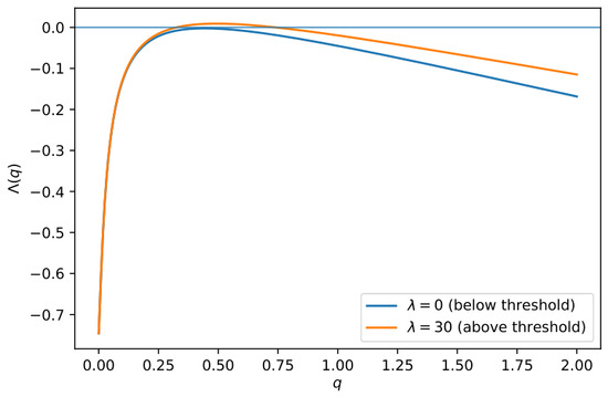
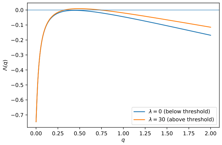
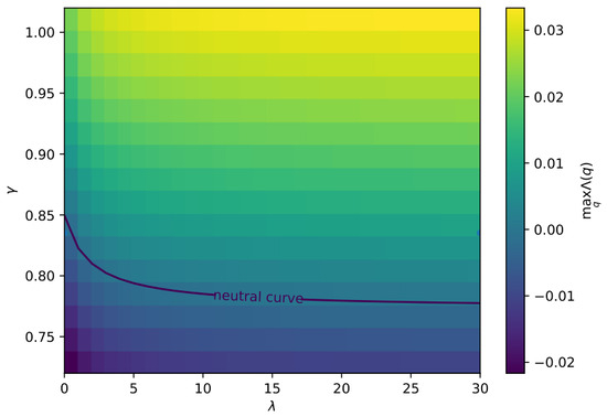
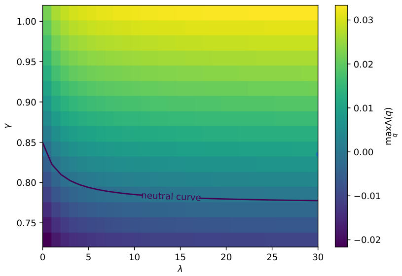
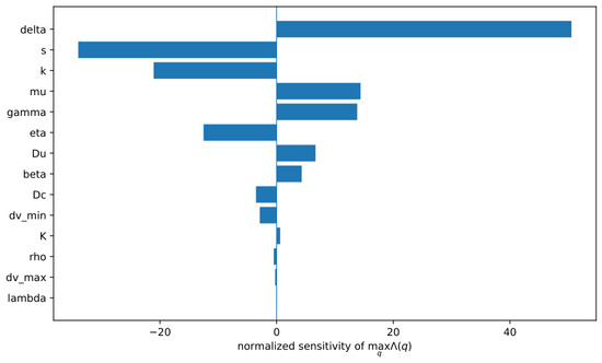
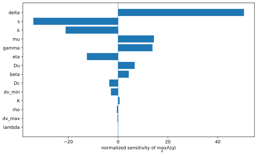
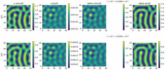
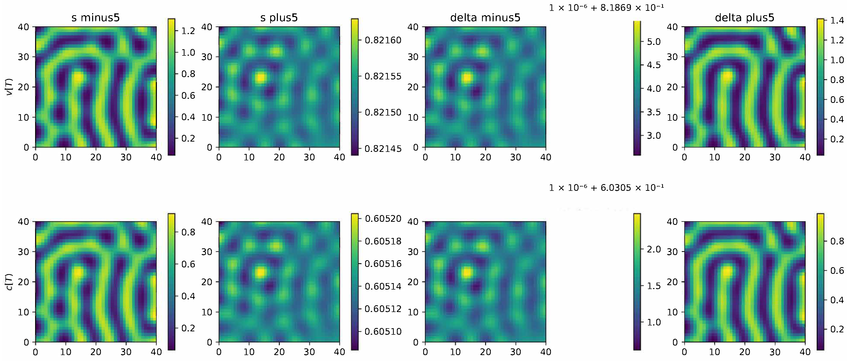
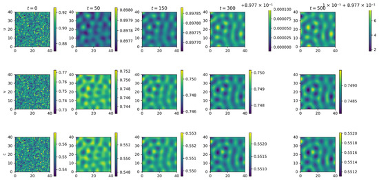
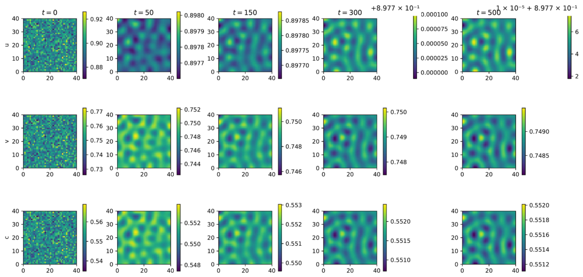
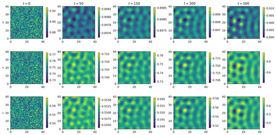
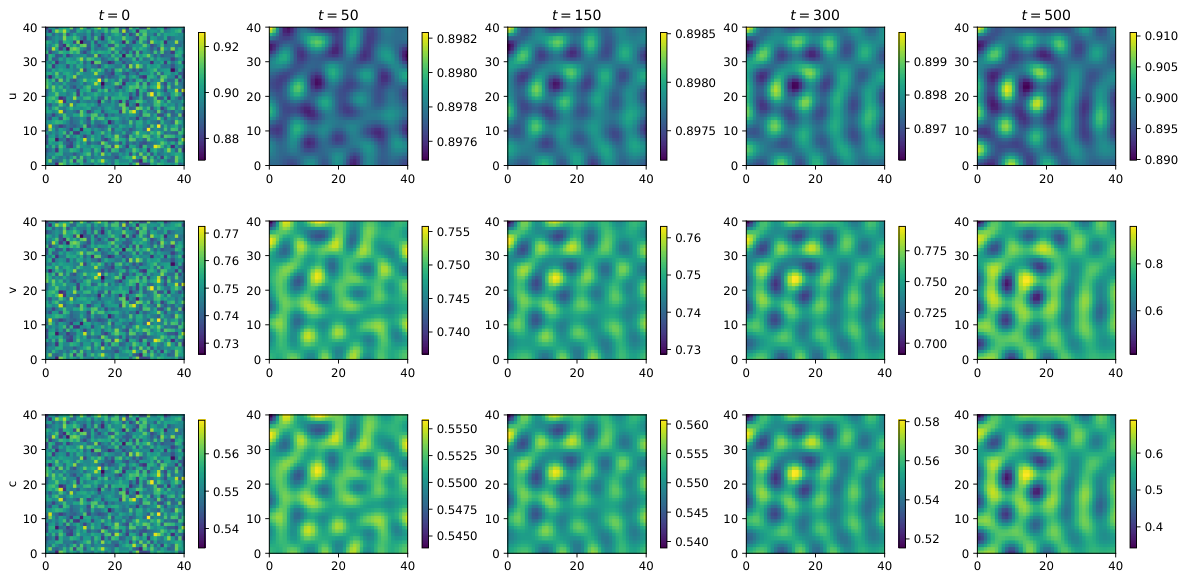
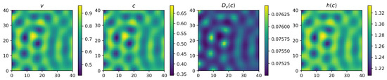
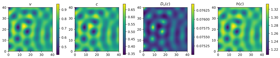
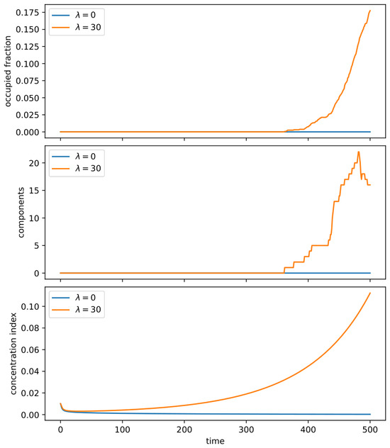
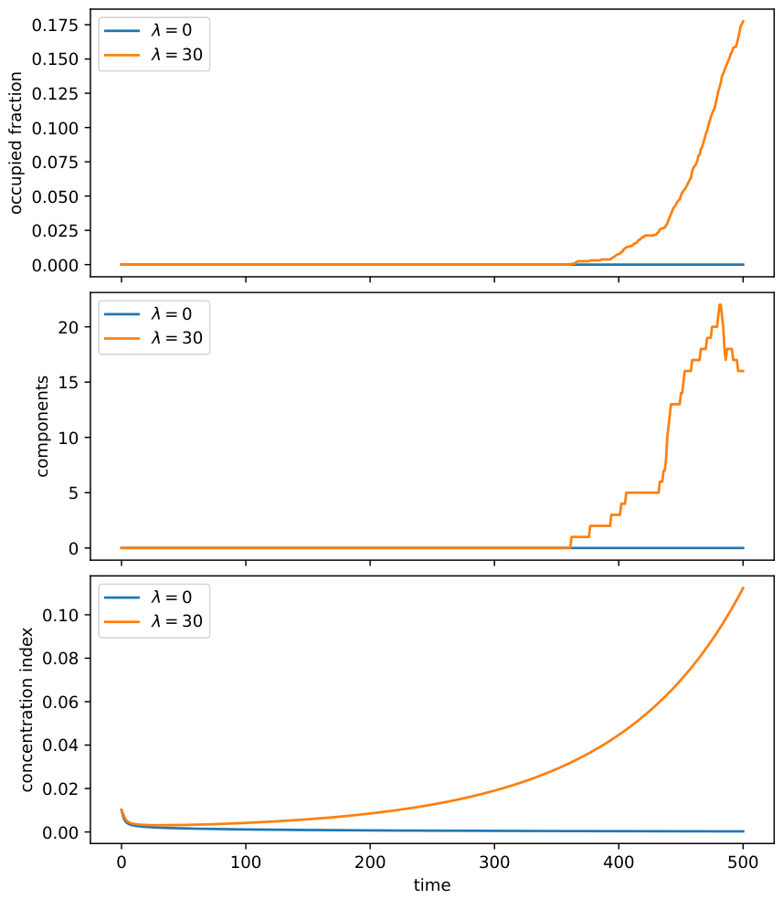
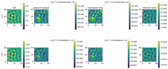
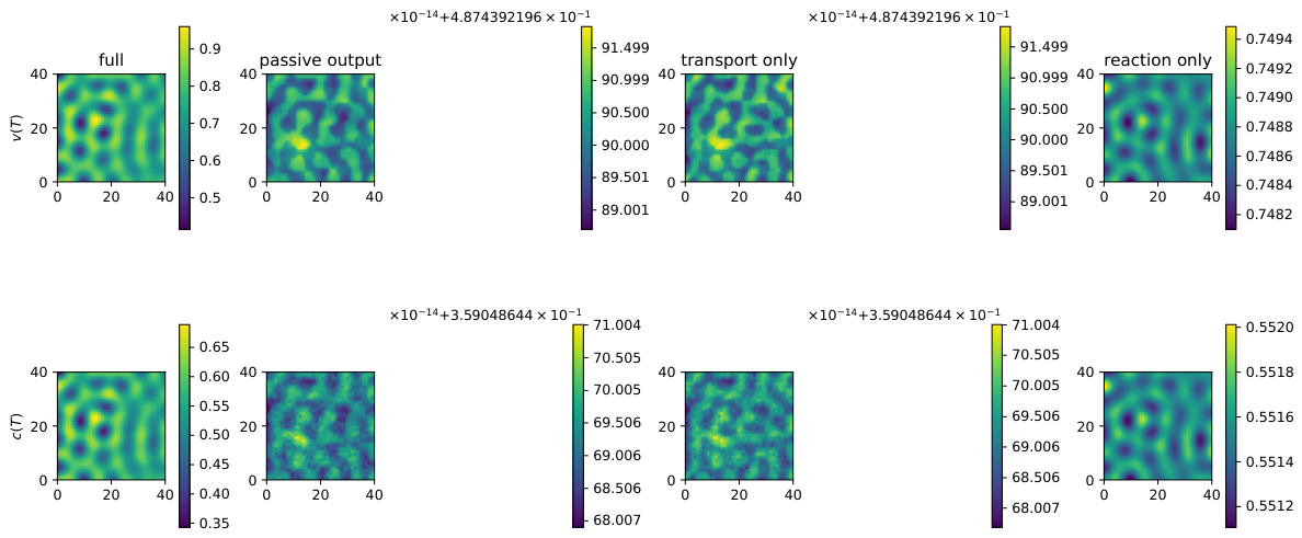
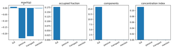
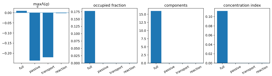
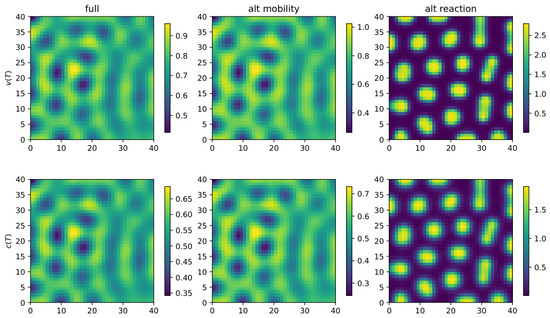
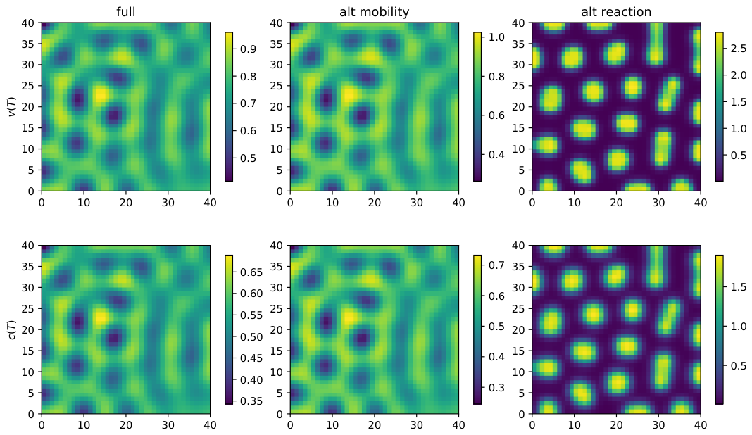

Disclaimer/Publisher’s Note: The statements, opinions and data contained in all publications are solely those of the individual author(s) and contributor(s) and not of MDPI and/or the editor(s). MDPI and/or the editor(s) disclaim responsibility for any injury to people or property resulting from any ideas, methods, instructions or products referred to in the content. |
© 2026 by the authors. Licensee MDPI, Basel, Switzerland. This article is an open access article distributed under the terms and conditions of the Creative Commons Attribution (CC BY) license.