Risk-Based Multi-Objective Approach for Improving Fairness of PV Curtailment in Low-Voltage Distribution Networks

Abstract

This paper proposes a risk-based, multi-objective approach to identify a solution, referred to as the fairness improvement plan, that enhances the fairness of photovoltaic (PV) curtailment, primarily applied to mitigate overvoltage issues in both balanced and unbalanced low-voltage distribution networks with high PV penetration. The proposed approach considers the uncertainty of loads, PV generation, and slack bus voltage. Relative Distance Measure (RDM) interval arithmetic is employed to represent these uncertainties while accounting for correlations among uncertain quantities, and the Pareto Simulated Annealing (PSA) method is used to generate a set of efficient fairness improvement plans. The Hurwicz criterion for measuring risk, which accounts for a decision maker’s risk preference, is incorporated in the interval TOPSIS technique to identify the fairness improvement plan, selected from a set of efficient plans, that minimizes the risk of financial losses and the risk of unfairness of PV’s active power curtailment. The numerical results obtained show that the proposed approach improves the insight and the understanding of the fairness improvement planning under uncertainty. They also highlight the effectiveness of incorporating decision makers’ risk preferences and their trade-off preferences between fairness and cost in developing the optimal fairness improvement plan under uncertainty in low-voltage distribution networks with high PV penetration.

1. Introduction

Due to the high penetration of residential photovoltaics (PVs) in recent years, operational planning and control in low-voltage distribution networks that most efficiently support PVs in everyday operations have become one of the main concerns for distribution system operators (DSOs). Different approaches are proposed for obtaining a solution that minimizes PV active power curtailment/reduction cost, hereafter referred to as PV curtailment, and satisfies operational (voltage and capacity constraints) constraints. A comprehensive review of these approaches proposed so far is presented in [1,2,3]. Among the proposed approaches, the optimization based offers the most efficient solution due to the system-wide awareness and the PV’s statuses [1,3,4]. The fair distribution of PV curtailment, which enables a PV with an equal opportunity to produce electricity and share the responsibility of voltage regulation, is considered by several optimization-based approaches [5,6,7,8,9,10,11,12,13]. A distributed optimal power flow formulation is proposed in [5] to incorporate fairness in curtailing PV generation. Future loads, generation form PVs, and the slack bus voltage in [5] are considered precisely known and, thus, are described by crisp (deterministic) values. In [6], a linearized, three-phase optimal power flow-based approach with different fairness perspectives is proposed to obtain the best fairness improvement plan. It also considers that all input quantities are precisely known. The linearized optimal power flow-based method to obtain the best fairness improvement plan is also proposed in [7], where all input parameters are described by crips (deterministic) values. In [8], a sensitivity-based analytical approach for fair PV curtailment, along with neutral current compensation, is proposed. To find a solution that provides a fair PV curtailment plan, proposed algorithms, which employ power flow analysis and real-time measurements, are iterated several times to determine the fair PV curtailment plan.

The approaches in [5,6,7,8] consider that all inputs are precisely known, but they are often assessed with some uncertainty for many reasons. The loads (consumption) in a low-voltage network can only be roughly predicted. The same is the case with the PV’s generation and the slack bus voltage (e.g., voltage at the low-voltage busbar in a substation). In the presence of uncertainties, various combinations of input parameters (loads, PV generation, and slack bus voltages) may occur. Because of that, the approaches that do not consider uncertainty usually lead to poor quality solutions and solutions that may introduce operational risks in the network.

The approach proposed in [9] employs a bi-level framework that considers the uncertainty of loads and PV generation. It employs a second-order cone relaxation of the power flow equations and the probabilistic constraints within the robust optimization concept to determine the best fairness improvement plan. In [10], a linearized unbalanced three-phase optimal power flow model is used within the robust optimization framework to obtain a robust fairness improvement plan considering the uncertainty in power consumption and production. In [11], a deterministic procedure is proposed, which also employs a linearized unbalanced three-phase optimal power flow model, for obtaining the robust fairness improvement plan in the presence of load and PV generation uncertainty. In [12], the linearized power flow model is used in the proposed fairness-incorporated online feedback optimization approach. It uses a set of integrated real-time measurements and is intended to work in real time as a corrective tool. It is stated that the approach can be used for offline optimization, but the handling of uncertainties in input quantities is not addressed. In [13], a simulated annealing-based approach that considers the fairness of PV’s active power curtailment and the uncertainty in loads and PV generation is proposed. It employs the Equal Likelihood criterion for measuring risk and the classical TOPSIS (Technique for Order Preferences by Similarity to an Ideal Solution) method to obtain the best solution.

Approaches [9,10,11,12] employ robust optimization concepts to determine the best fairness improvement plan. However, the robust optimization formulation is inherently worst case and, thus, usually leads to too-conservative solutions [11,14]. In addition, approaches [9,10,11,12,13] do not address properly the financial and operational risks that DSOs and PVs can face due to the uncertainty in input quantities. Consequently, a decision maker’s risk preferences cannot be considered in obtaining the best fairness improvement plan. Moreover, the proposed approaches do not consider the uncertainty in slack bus voltage and the dependencies (correlations) between loads of different categories (e.g., households, commercial, and small industries); between PVs; and between loads and PVs [15,16], which influence the quality of the obtained solution [17].

Further, approaches [5,6,7,8,9,10,11,12] consider the fairness improvement planning problem as a single-criterion optimization problem. However, the fairness improvement problem considers multidimensional criteria (e.g., fairness, which is dimensionless [18], and costs). Accordingly, a goal is to find a plan that ensures the best balance between the fairness of PV curtailment and the costs according to a decision maker’s trade-off preference between fairness and cost aligned with the local policies concerning energy justice [19]. Finally, most of the proposed approaches use linearization or relaxation of the nonlinear power flow equations, which may lead to ineffective solutions [11,20].

This paper proposes a risk-based, multi-objective approach for fairness improvement planning in low-voltage distribution networks with high PV penetration. The approach is applicable to both balanced and unbalanced networks and incorporates uncertainties related to loads, PV generation, and slack bus voltage. In such an uncertain environment, the goal of DSOs is to define a fairness improvement plan that simultaneously minimizes the risk of financial losses (costs) and the unfairness of PV curtailment, ensuring fair distribution of active power curtailments among PVs. The approach considers both the cost of PV curtailment and penalties associated with voltage violations. Uncertain quantities are represented using intervals defined through Relative Distance Measure (RDM) arithmetic [21], and their possible values are analyzed while accounting for correlations among them. For each feasible combination of interval values, a set of effective solutions to the multi-objective fairness improvement problem is generated using the proposed Pareto Simulated Annealing (PSA) algorithm, which accounts for both active power curtailment and the reactive power capability of PVs. Each fairness improvement plan is then evaluated across all feasible combinations of interval quantities, resulting in interval-valued costs and unfairness. The plans are evaluated using the interval TOPSIS method that incorporates the Hurwicz criterion for risk assessment, enabling the ranking process to reflect the decision maker’s risk preferences. In this way, an optimal fairness improvement plan is obtained that minimizes the risk of financial losses and PV curtailment unfairness, in accordance with the decision maker’s risk preference and their trade-off between fairness and cost.

The main contributions of the paper can be summarized as follows:

-

Defines a risk-based multi-objective decision-making framework that simultaneously considers fairness in PV curtailment, curtailment costs, and penalties for voltage violations under uncertainties in load, PV generation, and slack bus voltage while accounting for correlations among uncertain quantities to determine the optimal fairness improvement plan in PV-rich low-voltage networks.

-

Designs a Pareto Simulated Annealing (PSA) algorithm to generate a set of efficient fairness improvement plans within the proposed risk-based framework.

-

Proposes an interval TOPSIS method that applies the Hurwicz criterion for risk assessment to rank efficient plans and select the optimal one, thereby incorporating the decision maker’s risk preferences.

-

Provides decision makers with a robust framework for defining fairness improvement plans that achieve an optimal balance between fairness in PV curtailment and associated costs from voltage violations and curtailment while reflecting trade-off preferences between fairness and costs, aligned with local energy justice policies [19], and the decision maker’s risk attitude.

The rest of the paper is organized as follows. Section 2 describes the modeling of the uncertain quantities (loads, PV generation, and slack bus voltage) in low-voltage networks using RDM interval arithmetic. Section 3 presents a risk-based approach for determining the optimal fairness improvement plan, based on the decision maker’s risk preferences and the trade-off between fairness and cost. Section 4 presents numerical case studies that demonstrate the efficiency and effectiveness of the proposed approach, while Section 5 concludes the paper.

2. Uncertainty Modeling of Input Quantities

Many input parameters, such as loads, PV generation, and slack bus voltage, that form the basis for studies of low-voltage networks with high PV penetration are subject to significant uncertainty, primarily due to incomplete or imprecise information [22,23]. Interval arithmetic-based approaches have proven efficient and provide valuable insights when dealing with such uncertainties [17,24,25,26]. Accordingly, in this study, uncertainties in load, PV generation, and slack bus voltage are represented using intervals. The load uncertainty is modeled as the interval $\stackrel{\mathrm{-}}{\mathrm{D}}(k) = [{\mathrm{D}}_{\mathrm{L}}(k), {\mathrm{D}}_{\mathrm{R}}(k)$], as shown in Figure 1. This interval is represented using interval Relative Distance Measure (RDM) arithmetic. Interval RDM arithmetic ensures that arithmetic operations on intervals do not produce overly pessimistic results (overestimated intervals) [17,21]. It also guarantees correct realization of arithmetic operations for all types of correlations among interval quantities [17]. The representation of load uncertainty using RDM arithmetic is as follows:

$$\stackrel{\mathrm{-}}{\mathrm{PD}}(k){=\mathrm{PD}}_{\mathrm{L}}(k)+{\beta }_{\mathrm{D}\left(k\right)}·(\mathrm{P}{\mathrm{D}}_{\mathrm{R}}\left(k\right)-\mathrm{P}{\mathrm{D}}_{\mathrm{L}}(k))=\mathrm{P}{\mathrm{D}}_{\mathrm{L}}(k){+\beta }_{\mathrm{D}\left(k\right)}·\mathrm{\Delta }\mathrm{PD}\left(k\right), { \beta }_{\mathrm{D}\left(k\right)}\in \left[\mathrm{0,1}\right]$$

(1)

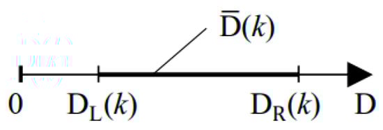
Figure 1. Interval-valued load D at node (k).

Similarly, the uncertainty of PV generation is expressed as

$$\stackrel{-}{\mathrm{PPV}}(k)={\mathrm{PPV}}_{\mathrm{L}}(k)+{\beta }_{\mathrm{PV}\left(k\right)}·{(\mathrm{PPV}}_{\mathrm{R}}\left(k\right)-{\mathrm{PPV}}_{\mathrm{L}}\left(k\right))={\mathrm{PPV}}_{\mathrm{L}}(k){+\beta }_{\mathrm{PV}\left(k\right)}·\mathrm{\Delta }\mathrm{PPV}\left(k\right), {\beta }_{\mathrm{PV}\left(k\right)}\in \left[\mathrm{0,1}\right]$$

(2)

Expressions (1) and (2) represent the uncertainties in the active power of loads and PV generation, respectively. The uncertainties in reactive power, $\stackrel{\mathrm{-}}{\mathrm{QD}}(k)$ and $\stackrel{\mathrm{-}}{\mathrm{QPV}}(k)$, can be modeled in a similar manner. By adjusting the β values within the range [0, 1], various scenarios of load and PV generation, representing different states of nature, can be simulated.

The slack bus, also called the balancing node, is a single node where the voltage magnitude and phase angle are fixed. It acts as the reference node in power flow analysis, ensuring the balance between total generation and total demand, including power losses. The uncertainty of the slack bus voltage (V₀) in a low-voltage network (e.g., voltage at the low-voltage busbar in a substation) is described as follows:

$$\stackrel{\mathrm{-}}{{\mathrm{V}}_0}={\mathrm{V}}_{0,\mathrm{L}}+{\beta }_V·({\mathrm{V}}_{0,\mathrm{R}}-{\mathrm{V}}_{0,\mathrm{L}}), {\theta }_0=0, {\beta }_V\in \left[\mathrm{0,1}\right]$$

(3)

These intervals can be established based on expert knowledge and are supported by data obtained from field measurements [15,27,28]. Due to the interdependence among various load types, photovoltaics (PVs), and the interactions between loads and PVs [15,16], not all combinations of their interval values are considered, only those permitted by the defined interdependence relations. The interdependence between intervals $\stackrel{\mathrm{-}}{\mathrm{a}}$and $\stackrel{\mathrm{-}}{\mathrm{b}}$, characterized by constraints on their admissible pairings, can be represented using the following relation [17,24]:

$$\begin{gathered} \mathrm{D}\mathrm{P}(r)=\left\{\left({\beta }_a,{\beta }_b\right):\mathit{max}(0,-{\beta }_a-r,{\beta }_a-1+r)\le {\beta }_b\right.\left.\le \\ \hspace{1em}\hspace{1em}\hspace{1em}\hspace{1em}\hspace{1em}\hspace{1em}\hspace{1em}\hspace{1em}\hspace{1em}\hspace{1em}\mathit{min}(1,{\beta }_a+1-r,-{\beta }_a+2+r),{\beta }_a \bigwedge { \beta }_b\in \left[\mathrm{0,1}\right]\right\} \end{gathered}$$

(4)

Relation (4) establishes that a dependency exists for each value of the correlation coefficient r, where $r\in [-1, 1]$. It specifies the feasible combinations of interval quantities corresponding to the given correlation coefficient. The correlation coefficients among PVs, among loads, and between PVs and loads can be determined through statistical analysis and by examining scatter plots of the uncertain quantities derived from measurement data [24,27,28]. Furthermore, analyzing these scatter plots enables the identification of a suitable dependence model that captures the interrelationships between the uncertain variables [24]. It is noteworthy that the number of feasible combinations of intervals$\stackrel{\mathrm{-}}{\mathrm{a}}$and $\stackrel{\mathrm{-}}{\mathrm{b}}$, as defined by Relation (4), and consequently, the computational burden of interval analysis is significantly influenced by the degree of dependence between the intervals, expressed through the correlation coefficient r [17].

3. Risk-Based Multi-Objective Solution Approach

In the presence of uncertainty in load, PV generation, and slack bus voltage, the goal is to improve the fairness of PV curtailment by finding a fairness improvement plan that responds most efficiently to any plausible combination of uncertain inputs, i.e., a plan that minimizes the risk of financial losses (penalties due to voltage violations and cost of PV curtailment) and the risk of unfairness in PV curtailment.

The minimum risk solution to the fairness improvement problem under uncertainty in low-voltage networks is determined as follows. For each time period within the planning horizon (e.g., each hour in a 24-h schedule), possible states of nature, defined as feasible combinations of the uncertain quantities (loads, PV generation, and slack bus voltage), are generated within the procedure described in Section 3.1. The multi-objective fairness improvement problem for each state of nature is defined in Section 3.2. The Pareto Simulated Annealing algorithm, presented in Section 3.3, is employed to generate a set of efficient fairness improvement plans for each feasible state of nature. These plans are then evaluated across all feasible states of nature, as described in Section 3.4. Based on this evaluation, the minimum risk solution for the considered time period is determined using the interval TOPSIS method introduced in Section 3.5.

The flowchart in Figure 2 summarizes the proposed approach.

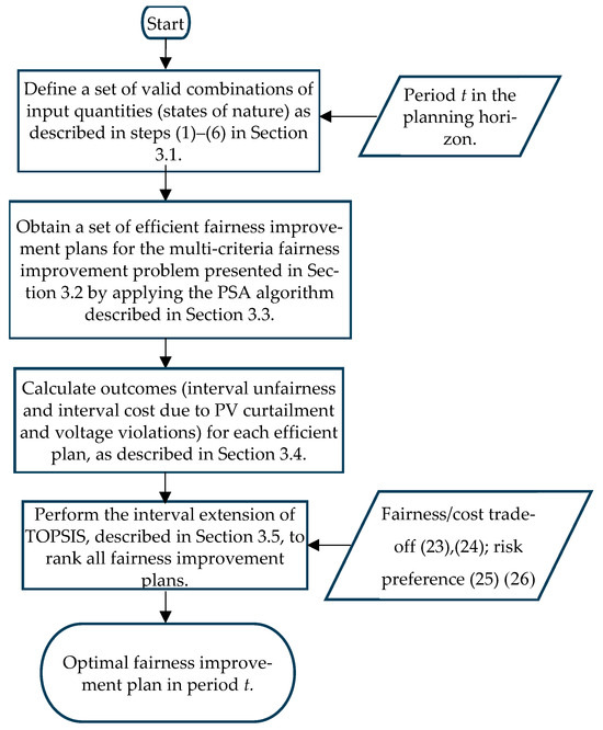
Figure 2. Flowchart of the solution approach.

3.1. Procedure for Deriving Efficient Fairness Improvement Plans

The procedure for determining efficient fairness improvement plans under uncertainty is as follows:

(1)

Choose a time t within the overall planning period (e.g., a specific hour in a 24-h schedule).

(2)

Define the following feasible combinations of $\beta (t)$ values for uncertain quantities:

-

${ \beta }_{D(k)}(t)$ values for loads are determined using Relation (4), the correlation coefficient between different types of loads (e.g., correlation coefficient $r_{R,C }(t)$ between residential and commercial loads), and the correlation coefficient between loads and PVs ($r_{D,\mathit{PV}}(t)$). A perfect positive correlation ($r_{D }(t)$= 1) is assumed between loads of the same type, as well as between active and reactive power consumption.

-

${\beta }_{\mathrm{P}\mathrm{V}\left(\mathrm{k}\right)}(t)$ values for PVs are determined using Relation (4), the correlation coefficient between PVs ($r_{\mathrm{P}\mathrm{V}}(t)$), and the correlation coefficient between loads and PVs (($r_{D,\mathit{PV}}(t)$). A perfect positive correlation between PVs is assumed.

(3)

Choose a feasible combination of ${ \beta }_{D(k)}(t)$, ${ \beta }_{\mathit{PV}(k)}(t)$, and ${\beta }_V(t)$ values and compute the corresponding crisp values for interval loads, PV generation, and slack bus voltage using Equations (1)–(3). The slack bus voltage is assumed to be uncorrelated with both loads and PVs.

(4)

For the obtained crisp values of interval quantities, determine a set of efficient solutions to the nonlinear multi-objective fairness improvement problem (5)–(18) formulated in Section 3.2. This set is generated using the proposed Pareto Simulated Annealing (PSA) algorithm, as detailed in Section 3.3.

(5)

Return to step (3).

(6)

Continue iterating step (5) until all feasible combinations of ${ \beta }_{D(k) }(t)$, ${ \beta }_{\mathit{PV}(k)}(t)$, and ${\beta }_V(t)$ have been evaluated.

(7)

The above procedure enables the derivation of a set of efficient fairness improvement plans, denoted as S_Pareto, which represents the union of efficient solutions obtained in step (6) for each feasible combination of β values. Note that this procedure is applied in each period in the considered planning horizon (e.g., in each hour of 24-h planning horizon).

3.2. Formulation of Multi-Objective Fairness Improvement Problem

The multi-objective fairness improvement problem in low-voltage networks is described by Equations (5)–(18). The crisp values of the interval-valued load, interval-valued PV generation, and interval-valued slack bus voltage, obtained for particular values of ${ \beta }_{D(k) }(t)$, ${ \beta }_{\mathit{PV}(k)}(t)$ and ${\beta }_V(t)$, are depicted by ${}^{\beta }PD(.), {}^{\beta }PPV(.)$ and ${}^{\beta }{V}_0,$ respectively, in (5)–(18). Hence, the superscript β indicates that the optimization problem (5)–(18) is solved for a feasible combination of the interval-valued input parameters.

(a)

Objective function

$$min \left\{{}^{\beta }CC,{}^{\beta }CV, {}^{\beta }Unf \right\}, \beta \equiv \left\{{\beta }_D, {\beta }_{\mathit{PV}},{\beta }_V\right\}, \left({\beta }_D,{\beta }_{\mathit{PV}}, { \beta }_V\right)ϵ\left[\mathrm{0,1}\right]$$

(5)

$${}^{\beta }CC={\sum }_{i\in NPV}\{{}^{\beta }PPV(i)·\left(1-{}^{\beta }xpv\left(i\right)\right)·{CPV}_i·∆\mathrm{t}\}$$

(6)

$${}^{\beta }CV={\sum }_{i\in NN}{}^{\beta }vc(i)$$

(7)

$${}^{\beta }vc(i)=\left\{\begin{array}{c}{k}_v·{\left({}^{\beta }{v}_i-V_{max}\right)}^2, k_{max}·V_{max} \ge {}^{\beta }{v}_i>V_{max}\hfill \\ B, {{}^{\beta }v}_i>k_{max}·V_{max} \hfill \\ 0,{{ V}_{max}\ge {}^{\beta }v}_i\ge V_{min} \hfill \end{array}\right.,$$

(8)

$${}^{\beta }Unf={\sum }_{i\in NPV}{\sum }_{\begin{array}{c}m\in NPV\\ m=i+1\end{array}}{\left({}^{\beta }xpv\left(i\right)-{}^{\beta }xpv\left(m\right)\right)}^2$$

(9)

$${}^{\beta }xpv\left(i\right)={}^{\beta }ppv\left(i\right)/{}^{\beta }\mathrm{P}\mathrm{P}\mathrm{V}(i) ,i\in \mathrm{N}\mathrm{D}\mathrm{G}$$

(10)

The multi-objective function, which considers the cost of PV curtailment (${}^{\beta }CC$), the cost (penalties) due to voltage violations (${}^{\beta }CV$), and the unfairness of PV curtailment (${}^{\beta }Unf$), is given by Expression (5). The cost of PV curtailment, which lasts for ∆t hours, is described by (6). Penalties due to voltage limit violation are described by (7) and (8), whereas the unfairness of PVs’ curtailment is described by (9) and (10).

(b)

Constraints

$${ {}^{\beta }v}_i·{\sum }_{jϵN\left(i\right)}{ {}^{\beta }v}_j·\left(g_{ij}{cos{\theta }_{ij}}^{\beta }+b_{ij}{sin{\theta }_{ij}}^{\beta }\right)={}^{\beta }ppv\left(i\right)-{}^{\beta }PD\left(i\right), i\in \mathrm{N}\mathrm{N}$$

(11)

$${ {}^{\beta }v}_i·{\sum }_{jϵN\left(i\right)}{ {}^{\beta }v}_j·\left(g_{ij}{sin{\theta }_{ij}}^{\beta }-b_{ij}{cos{\theta }_{ij}}^{\beta }\right)={}^{\beta }qpv\left(i\right)-{}^{\beta }QD\left(i\right), i\in \mathrm{N}\mathrm{N}$$

(12)

$${ {}^{\beta }p}_{ij}={\left|{ {}^{\beta }v}_i\right|}^2·g_{ij}+\left|{ {}^{\beta }v}_i\right|·\left|{ {}^{\beta }v}_j\right|·[b_{ij}{sin{\theta }_{ij}}^{\beta }-g_{ij}{cos{\theta }_{ij}}^{\beta }], (i, j)\in \mathrm{N}\mathrm{N}$$

(13)

$${ {}^{\beta }q}_{ij}={\left|{ {}^{\beta }v}_i\right|}^2·b_{ij}-\left|{ {}^{\beta }v}_i\right|·\left|{ {}^{\beta }v}_j\right|·[g_{ij}{sin{\theta }_{ij}}^{\beta }+b_{ij}{cos{\theta }_{ij}}^{\beta }], (i, j)\in \mathrm{N}\mathrm{N}$$

(14)

$${{ {}^{\beta }p}_{ij}}^2+{{ {}^{\beta }q}_{ij}}^2\le S_{max}^2(i, j)\in \mathrm{N}\mathrm{N}$$

(15)

$${{}^{\beta }ppv\left(i\right)}^2+{}^{\beta }qpv{\left(i\right)}^2\le {SPV}_{i,max}^2, i\in \mathrm{N}\mathrm{D}\mathrm{G}$$

(16)

$$V_{min }{\le {}^{\beta }v}_i\le {k_{max}·V}_{max}, i\in \mathrm{N}\mathrm{N}$$

(17)

$${}^{\beta }qpv(i)\le Q_{max}(i)$$

(18)

Equation (11) describes the active power balance at each node in the network for a combination of β values of interval quantities, described in Section 3.1, considering the possibility of active power curtailment of PVs (${}^{\beta }xpv )$. The reactive power balance at each node is given by (12). Equations (13) and (14) describe active and reactive power flow over the lines in the considered network. The thermal capacity of lines is described by (15). Equation (16) represents the capability curves of PVs, whereas (17) defines voltage constraints. Finally, (18) describes the reactive power absorption capability of a PV at node (i).

3.3. Pareto Simulated Annealing (PSA) Algorithm

The Pareto Simulated Annealing (PSA) algorithm, which incorporates the Q(V) and P(V) control actions of PVs, is proposed to identify the set of efficient solutions to the nonlinear multi-objective problem defined by Equations (5)–(18). The algorithm builds upon the technique introduced in [29] and is specifically tailored to address fairness improvement planning problems.

In the initial stage, the ranges of reactive power absorption for Q(V) control and active power curtailment for P(V) control, which will be explored within the PSA algorithm, are defined as follows:

• The following β values of interval quantities are considered: the right endpoints (${\beta }_{\mathrm{PV}\left(\mathrm{k}\right)}=1$) of interval active power of PVs and the right endpoint (${\beta }_V=1$) of the slack bus voltage. All interval loads are set to zero. PVs inject power at unity power factor.
• The following control actions are considered:

  (a)

  Q(V) control. The reactive power absorption range for each PV is defined as ∆Q $\in$[0, Q_max], where Q_max represents its maximum reactive power absorption capacity.

  (b)

  P(V) control. Active power output of every PV is curtailed by the same amount (percentage), e.g., by ∆p [%] = 1% of its forecasted power. A power flow calculation [30] is then performed, and voltage constraint violations are checked. If any violations persist, the active power output of each PV is further curtailed by the same predefined increment (e.g., by ∆p [%] = 1%). This iterative process continues until all voltage violations are resolved. The total curtailment applied to each PV is denoted as ∆P_max. Consequently, the range of active power curtailment to be explored for each PV within the PSA algorithm is defined as ∆P $\in$[0, ∆P_max].

The PSA algorithm for fairness improvement planning problems consists of the following steps:

(1)

Define a set of initial solutions ^βSIS_Initial as follows:

(1.1)

I. Select by chance a PV from the set of all PVs $\mathrm{\Pi }$. Select by chance type of control, P(V) or Q(V) control, and perform the following:

(a)

Q(V) control. Select by chance the percentage of reactive power absorption from the interval ∆Q, which is defined in step ii (a).

(b)

P(V) control. Select by chance the percentage of active power curtailment from the interval ∆P, which is defined in step ii (b).

(1.2)

Calculate the power flow for the solution obtained in step (1.1). Based on the results, compute the cost of PV curtailment, the cost of voltage violation penalties, and the unfairness using Expressions (6)–(9) and (16).

(1.3)

Repeat steps (1.1) and (1.2) until set $\mathrm{\Pi }$ is exhausted. This process yields an initial (candidate) fairness improvement plan.

(1.4)

Repeat steps (1.1)–(1.3) a total of (K_Initial x NPV) times, where NPV is the number of PVs in set $\mathrm{\Pi }$, and K_Initial is a constant greater than or equal to 1. In this way, the initial set of fairness improvement plans ^βSIS_Initial is defined.

(2)

Define the initial temperature T_max and the minimum temperature T_min (stopping criterion). Set k = 1 for the iteration index.

(3)

Select a candidate solution S_c from the set ^βSIS_Initial. Then, identify the solution ${\mathbf{S}}_{\mathrm{c}\mathrm{l}}\in {}^{\beta }{\mathrm{S}\mathrm{I}\mathrm{S}}_{\mathrm{I}\mathrm{n}\mathrm{i}\mathrm{t}\mathrm{i}\mathrm{a}\mathrm{l}}$ that is closest to S_c and non-dominated with respect to it. If no such solution S_cl exists, or it is the first iteration involving S_c, the weights ${\lambda }_{CC}{, \lambda }_{CV}$, and ${\lambda }_{UF}$ are randomly assigned, such that ${\lambda }_{CC}+{\lambda }_{CV}+{\lambda }_{UF}=1$. Otherwise, the weights for each objective are calculated as follows:

$${\lambda }_j=\left\{\begin{array}{c}\mu ·{\lambda }_j^{{\mathit{S}}_c} if f_j({\mathit{S}}_c)\ge f_j({\mathit{S}}_{cl})\\ {\lambda }_j^{{\mathit{S}}_c}/\mu if f_j({\mathit{S}}_c)<f_j({\mathit{S}}_{cl})\end{array}\right., f_j\in \left\{{}^{\beta }CC,{}^{\beta }CV, {}^{\beta }Unf\right\},\hspace{1em}j\in \{CC,CV,UF\}$$

(19)

The weights in (19) are normalized, such that $\sum _j{\lambda }_j=1$. The parameter μ > 1 is a constant close to one (e.g., μ = 1.05). The terms ${\lambda }_{CC }^{{\mathit{S}}_c}{,\lambda }_{CV}^{{\mathit{S}}_c}$, and ${\lambda }_{UF}^{{\mathit{S}}_c}$ represent the weights used in the previous iteration for the solution ${\mathit{S}}_{\mathit{c}}$.

(4)

Select by chance a PV from set $\mathrm{\Pi }$. Then, choose by chance the type of control, either P(V) or Q(V) control, and proceed with the following:

(a)

Q(V) control. Select by chance the percentage of reactive power absorption from the interval ∆Q, which is defined in step ii (a).

(b)

P(V) control. Select by chance the percentage of active power curtailment from the interval ∆P, which is defined is step ii (b).

As a result, a neighborhood solution S_new is obtained. The selected PV is then removed from set $\mathrm{\Pi }$.

(5)

Calculate the power flow for the neighborhood solution S_new. Based on the results, compute the PV curtailment cost and voltage violation penalties, as well as the unfairness, using (6)–(9) and (16). Then, apply the following acceptance rules.

If the solution S_new dominates S_c, it is accepted and added to the set of efficient solutions ^βS_Pareto. Otherwise, the candidate solution is accepted with the following probability:

$$\begin{gathered} \hspace{1em}\hspace{1em}\hspace{1em}\hspace{1em}\hspace{1em}\hspace{1em}\hspace{1em}\hspace{1em}\hspace{1em}\hspace{1em}\hspace{1em}\hspace{1em}\hspace{1em}\hspace{1em}\hspace{1em}\hspace{1em}\hspace{1em}\hspace{1em}\hspace{1em}\hspace{1em}\hspace{1em}\hspace{1em}\mathrm{P}\left(Accept {\mathit{S}}_{new}\right)= \mathit{min}\left\{1;exp\left({\displaystyle \frac{{\lambda }_{CC}·\left(CC({\mathit{S}}_{\mathit{c}})-CC({\mathit{S}}_{new})\right)}{T_k}}+{\displaystyle \frac{{\lambda }_{CV}·\left(CV({\mathit{S}}_{\mathit{c}})-CV({\mathit{S}}_{new})\right)}{T_k}}+ \\ {\displaystyle \frac{{\lambda }_{UF}·\left(Unf({\mathit{S}}_{\mathit{c}})-Unf({\mathit{S}}_{new})\right)}{T_k}}\right)\right\} \end{gathered}$$

(20)

If P(Accept S_new) > random [0, 1], the solution S_new is accepted, i.e., it becomes the current solution S_c. Otherwise, if P(Accept S_new) < random [0, 1], the neighborhood solution is rejected.

(6)

If set $\mathrm{\Pi }$ is not yet exhausted, return to step (4). Otherwise, proceed to step (7).

(7)

If the set ^βSIS_Initial is not yet exhausted, return to step (3). Otherwise, proceed to step (8).

(8)

Define the new temperature $T_{k+1}=\epsilon ·T_k$, where $\epsilon \in (0.5-0.99)$. If ${T_{k+1}<T}_{min}$, proceed to step (9). Otherwise, increase by increment the iteration index k by 1 and return to step (3).

(9)

The PSA algorithm is terminated, resulting in the set of fairness improvement plans ^βS_Pareto. From this set, non-dominated solutions are filtered to form the final output.

The proposed PSA algorithm generates a set ^βS_Pareto for each feasible combination of β values of input quantities, as described in Section 3.1. The union of these sets forms the overall Pareto set S_Pareto. Each plan in set S_Pareto is evaluated according to the procedure outlined in Section 3.4.

It is worth noting that the proposed PSA algorithm provides a high-quality approximation of the complete set of efficient solutions for relatively large multi-objective problems within a comparatively short computational time [29]. Furthermore, the algorithm’s inherent parallelism makes it well suited for parallel implementation, which can significantly reduce its solution time.

3.4. Determining the Optimal Fairness Improvement Plan

Each plan in set S_Pareto is evaluated by considering feasible states of nature as follows. For a given fairness improvement plan (j), and a feasible combination of ${ \beta }_{D(k)}(t)$, ${ \beta }_{\mathit{PV}(k)}(t)$, and ${\beta }_V(t)$ values, the cost of PV curtailment, the cost of voltage violation penalties, and the unfairness of PV curtailment are calculated. These calculations are based on the known values of PV active power curtailment and/or reduction due to reactive power absorption, i.e., the decision variables defined by plan (j). By performing these calculations across all feasible combinations of ${ \beta }_{D(k) }(t)$, ${ \beta }_{\mathit{PV}(k)}(t)$, and ${\beta }_V(t)$ values, the interval cost of PV curtailment ($\overline{{CC}_j}=[{CC}_{L,j}, {CC}_{R,j}]$)), the interval cost due to voltage violations ($\overline{{CV}_j}=[{CV}_{L,j}, {CV}_{R,j}]$), and the interval unfairness of PV curtailment (${\overline{Unf}}_j=[{Unf}_{L,j}, {Unf}_{R,j}]$) are obtained for a fairness improvement plan (j). In this way, interval costs and interval unfairness are obtained for each fairness improvement plan in set S_Pareto.

The optimal fairness improvement plan, which minimizes the risk of financial losses and unfair PV curtailment, is identified by ranking the plans in set S_Pareto based on their interval costs and interval unfairness. This ranking is performed using the interval TOPSIS method, as described in Section 3.5. The proposed interval TOPSIS method enables the ranking of interval-valued multi-objective solutions by incorporating the decision maker’s risk preferences, defined using the Hurwicz criterion for risk assessment [31,32], as well as their trade-off preferences between fairness and cost.

3.5. Interval TOPSIS

The interval TOPSIS employs the approach of direct interval extension of the TOPSIS method [33], which overcomes the drawbacks of other TOPSIS interval extensions [34,35,36]. However, unlike the approach in [33], the interval extension of TOPSIS proposed here incorporates the decision maker’s risk preferences by introducing the Hurwicz criterion for risk measurement in the ranking (comparison) of intervals. Its advantages are demonstrated in Appendix A. The interval TOPSIS procedure is as follows [37]:

(1)

Normalized interval ratings are computed as follows:

$$r_{mj}^L={\displaystyle \frac{f_{mj}^L}{\sqrt{\sum _{j=1}^J(f_{mj}^L{)}^2+(f_{mj}^R{)}^2}}}, m=1,\dots ,M, j=1, \dots , J$$

(21)

$$r_{mj}^L={\displaystyle \frac{f_{mj}^L}{\sqrt{\sum _{j=1}^J(f_{mj}^L{)}^2+(f_{mj}^R{)}^2}}}, m=1,\dots ,M, j=1, \dots , J$$

(22)

where $f_{mj}^L$ and $f_{mj}^R$ represent left and right endpoints, respectively, of the $m$^th interval objectives in the jth fairness improvement plan belonging to the set of all considered plans S_Pareto. J denotes the number of fairness improvement plans in set S_Pareto, and M represents the number of objectives. Since three interval objectives are considered M = 3, $f_{1j}^L$ corresponds to the left endpoint of the interval cost due to PV curtailment ${(CC}_{L, j}$), $f_{2j}^L$ to the cost due to voltage violation (${CV}_{L, j}$), and $f_{3j}^L$ to the left endpoint of interval unfairness (${Unf}_{L, j}$) in fairness improvement plan (j). The same applies to the right endpoints. The interval costs and interval unfairness for plan (j) are obtained as described in Section 3.4.

(2)

Weighted normalized interval ratings are computed as follows:

$$d_{mj}^L=w_m·r_{mj}^L, d_{mj}^R=w_m·r_{mj}^R$$

(23)

$${\sum }_{m=1}^M{w}_k=1$$

(24)

where w_k represents the weighting factors that reflect the decision maker’s preferences, i.e., trade-offs among the considered objectives (costs and unfairness).

(3)

Interval ideal (${\overline{I}}^{\mathrm{*}}$) and negative-ideal (${\overline{I}}^{-})$ alternatives are calculated as follows:

$$\begin{gathered} \hspace{1em}\hspace{1em}\hspace{1em}\hspace{1em}\hspace{1em}\hspace{1em}\hspace{1em}\hspace{1em}\hspace{1em}\hspace{1em}{\overline{I}}^{*}=\left\{[d_1^{*L}, d_1^{*R}], [d_2^{*L},d_2^{*R}],\dots ,[d_M^{*L},d_M^{*R}]\right\}=\underset{j}{\{\mathit{min}}[d_{mj}^L, d_{mj}^R], m\in \\ Cost; \underset{j}{\mathit{max}}[d_{kj}^L, d_{kj}^R], m\in Benefit\} , \end{gathered}$$

(25)

$$\begin{gathered} \hspace{1em}\hspace{1em}\hspace{1em}\hspace{1em}\hspace{1em}\hspace{1em}\hspace{1em}\hspace{1em}\hspace{1em}\hspace{1em}\hspace{1em}\hspace{1em}{\overline{I}}^{-}=\left\{[d_1^{-L}, d_1^{-R}], [d_2^{-L},d_2^{-R}],\dots ,[d_M^{-L},d_M^{-R}]\right\}=\{\underset{j}{\mathit{max}}[d_{mj}^L, d_{mj}^R], m\in \\ Cost; \underset{j}{\mathit{min}}[d_{mj}^L, d_{mj}^R], m\in Benefit\} \end{gathered}$$

(26)

In Expressions (25) and (26), the term ‘Cost’ refers to objectives intended for minimization, whereas the term ‘Benefit’ denotes objectives aimed at maximization. The ranking of intervals in Expressions (25) and (26) is conducted using the Hurwicz criterion, which facilitates interval-based evaluation in accordance with the decision maker’s attitude toward risk. For more details on the Hurwicz criterion, please refer to Appendix A and [31,32]. Accordingly, the interval ideal and negative-ideal alternatives are derived by ranking the interval-valued costs of PV curtailment, voltage violations, and unfairness across all considered plans, in alignment with the decision maker’s specified risk preferences and the trade-off preferences between costs and unfairness.

(4)

The separation measures between each fairness improvement plan and the ideal ($D_j^{\mathrm{*}}$), as well as the negative-ideal ($D_j^{-}$) alternative, are computed using the Euclidean distance in an n-dimensional space, as defined by the following expressions:

$$D_j^{*}= {\left\{ {\sum }_{m=1}^M(d_{mj}^R-d_k^{*R}{)}^2+{\sum }_{m=1}^M(d_{mj}^L-d_k^{*L}{)}^2\right\}}^{1/2}$$

(27)

$$D_j^{-}={\left\{ {\sum }_{m=1}^M(d_{mj}^R-d_k^{-R}{)}^2+{\sum }_{m=1}^M(d_{mj}^L-d_k^{-L}{)}^2\right\}}^{1/2}$$

(28)

(5)

The relative closeness of each fairness improvement plan to the ideal solution ($R_j^{\mathrm{*}}$) is determined using the following expression:

$$R_j^{*}={\displaystyle \frac{D_j^{-}}{D_j^{*}{+D}_j^{-}}}, j=1,\dots ,J$$

(29)

The fairness improvement plan (j) that yields the highest value of $R_j^{*}$ is considered the optimal solution.

4. Numerical Results

The proposed approach is tested on the low-voltage network presented in Figure 3 [38], which contains 20 customers with integrated PV systems. There are three types of residential customers (type 1, type 2, and type 3) and one type of commercial customers, with load and PV rated power data provided in Pavlos S. Georgilakis. The load data in Table 1 are obtained from [38] for a time of day when PV output is expected to be at its highest level (e.g., t = 13:00 h), whereas the rated power of the PVs is similar to that reported in [38]. It is assumed that the forecasted power consumption of each customer is represented by the interval $\stackrel{\mathrm{-}}{\mathrm{PD}}(k){ = [\mathrm{PD}}_{\mathrm{L}}(k),{ \mathrm{PD}}_{\mathrm{R}}(k)] =$ [0.85·Forecasted load, 1.15∙Forecasted load] and the forecasted PV generation is represented by the interval $\stackrel{\mathrm{-}}{\mathrm{PPV}}(k)={[\mathrm{PPV}}_{\mathrm{L}}(k), {\mathrm{PPV}}_{\mathrm{R}}(k)]=[0.55·\mathrm{R}\mathrm{a}\mathrm{t}\mathrm{e}\mathrm{d} \mathrm{p}\mathrm{o}\mathrm{w}\mathrm{e}\mathrm{r},\mathrm{R}\mathrm{a}\mathrm{t}\mathrm{e}\mathrm{d} \mathrm{p}\mathrm{o}\mathrm{w}\mathrm{e}\mathrm{r}]$. The power factor for loads is 0.9 inductive, while Q_max for PVs is 30% of the rated power. The intervals of load and generation reflect the level of (in)accuracy of load and PV forecasting in low-voltage networks [39,40]. The slack bus voltage is represented by the interval $\overline{\mathrm{V}}=\left[{\mathrm{V}}_{\mathrm{L}},{\mathrm{V}}_{\mathrm{R}}\right]=\left[0.392,0.416\right] \mathrm{k}\mathrm{V}$. Section and transformer data are provided in [38]. Other input parameters are as follows: cost of curtailment for all customers (${\mathrm{C}\mathrm{P}\mathrm{V}}_i$) is 1 [USD/kWh], $∆\mathrm{t}$ = 1 [h], ${\mathrm{V}}_{\mathrm{m}\mathrm{i}\mathrm{n}}=0.95·0.4$ [kV], ${\mathrm{V}}_{\mathrm{m}\mathrm{a}\mathrm{x}}=1.05·0.4$ [kV].

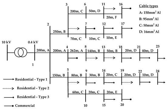
Figure 3. A 25-bus low-voltage network [38].

Table 1. Customer characteristics.

Type	Forecasted Load [kW]	PV [kW]
Residential—Type 1	1.2	13.0
Residential—Type 2	2.7	10.0
Residential—Type 3	1.8	11.0
Commercial	5.0	17.0

${\mathrm{k}}_{\mathrm{m}\mathrm{a}\mathrm{x}}=$ 1.05, and k_v = 1 [$/V]. The parameters ${ \beta }_{\mathrm{R}(k)}$, ${ \beta }_{\mathrm{C}(k)}$, ${ \beta }_{\mathrm{PV}(k)}$, and ${\beta }_{\mathrm{V}}$ belong to the set $\{0, 0.33, 0.66, 1\}$. Note that two different ${ \beta }_{\mathrm{D}(k)}$ parameters are considered, one (${ \beta }_{\mathrm{R}(k)}$) for residential customers and another (${ \beta }_{C(k)}$) for commercial customers. It is also assumed that the correlation coefficient between residential loads (type 1, type 2, and type 3) and the commercial loads is $r_{R,C}$ = −1, which ensures residential and commercial customers do not reach their peak loads simultaneously. A correlation coefficient of $r_{R,\mathit{PV}}$ = 0.5 is assumed between PVs and residential load. These values are consistent with those reported in [15,16]. In this way, 48 feasible combinations of the parameters ${ \beta }_{R(k)}$, ${ \beta }_{C(k)}$, ${ \beta }_{\mathit{PV}(k)}$, and ${\beta }_V$ are obtained, representing 48 distinct states of nature. Based on this, 748 fairness improvement plans are derived by applying the procedure described in Section 3.1. Six fairness improvement plans, labeled P1–P6, are discussed in the sequel. These plans are obtained by varying the weighting factors in (23) and the parameter $\delta$, as presented in Table 2. Here, $w$_C is the weighting factor for the cost of PV curtailment, $w$_P is the weighting factor for the cost of penalties due to voltage limits violation, and $w$_F represents the weighting factor for the unfairness of PVs curtailments. The parameter $\delta ϵ\left[\mathrm{0,1}\right]$ is used in the Hurwicz criterion to reflect the decision maker’s risk preference. When costs are considered, values of $\delta$closer to 1 indicate a risk-averse decision maker, while values closer to $0$ indicate a risk-seeking decision maker. For more details, please refer to Appendix A and [32]. Detailed results for plans P1–P6 are provided in Table 3 and Table 4.

Table 2. Definition of parameters for plans P1–P6.

Plan	P1	P2	P3	P4	P5	P6
$w$C	0.8	0.1	0.1	0.33	0.33	0.33
$w$F	0.1	0.8	0.1	0.33	0.33	0.33
$w$P	0.1	0.1	0.8	0.33	0.33	0.33
Correlation	yes	yes	yes	yes	no	yes
$\delta$	0.2	0.2	0.2	0.2	0.2	0.8

Table 3. Interval costs and unfairness.

Fairness Improvement Plan	P1	P2	P3	P4	P5	P6
Interval cost of PV curtailment [$]	[59.0, 60.0]	[106.5, 106.5]	[140.5, 145.8]	[88.4, 88.4]	[102.6, 103.7]	[76.3, 77.7]
Interval cost of voltage violations [$]	[10.3, 79.2]	[2.4, 25.2]	[0.72, 3.8]	[11.3, 39.0]	[5.2, 46.0]	[6.3, 57.4]
Interval unfairness of PV curtailment	[13.9, 31.3]	[0, 0]	[11.9, 22.1]	[4.7, 9.6]	[3.4, 7.8]	[5.3, 11.8]

Table 4. PV curtailment for plans P1–P4.

Node	P1		P2		P3		P4
	kW	% *	kW	% *	kW	% *	kW	% *
3	2.9	28.8	4.3	43.0	7.1	71.0	4.5	45.0
4	2.3	13.4	7.3	43.0	4.5	26.5	3.3	19.4
5	3.7	37.3	4.3	43.0	2.6	26.2	3.3	33.3
7	1.2	6.9	7.3	43.0	12.2	71.0	7.4	43.1
8	1.8	18.1	4.3	43.0	2.6	26.0	1.6	16.0
9	0.3	2.5	4.7	43.0	7.8	71.0	3.5	31.9
11	2.7	26.7	4.3	43.0	7.1	71.0	4.5	45.0
12	0.8	7.6	4.7	43.0	7.8	71.0	4.8	43.7
13	5.5	55.0	4.3	43.0	5.0	49.7	4.1	40.8
14	1.6	14.1	4.7	43.0	7.8	71.0	3.8	34.6
15	0.7	5.0	5.6	43.0	9.2	71.0	3.8	29.3
16	10.1	59.5	7.3	43.0	12.1	71.0	7.4	43.4
17	0.3	2.4	5.6	43.0	9.2	71.0	4.8	37.0
18	4.0	36.4	4.7	43.0	5.1	46.2	3.7	33.5
19	2.3	22.7	4.3	43.0	7.1	71.0	4.2	42.0
20	2.7	15.7	7.3	43.0	12.1	71.0	4.2	24.7
21	0.2	2.0	4.7	43.0	6.8	61.9	4.5	40.9
22	3.0	23.4	5.6	43.0	4.6	35.2	5.3	40.6
23	7.1	54.4	5.6	43.0	5.9	45.2	4.9	37.5
24	6.8	52.6	5.6	43.0	9.2	71.0	4.8	37.0
Total	60.0	/	106.5	/	145.8	/	88.4	/

* Percentage of rated power.

Plan P1 represents the optimal solution for a risk-averse decision maker, characterized by $\delta =0.2$, who values the cost of PV curtailment more than the fair distribution of PV curtailment or the penalties due to voltage violations. Results in Table 3 and Table 4 show that Plan P1 yields the lowest PV curtailment compared to the other plans. However, it also exhibits the highest interval unfairness in PV curtailment and the highest interval cost due to voltage violations among plans P1–P6.

Plan P2 represents the optimal solution for a risk-averse decision maker who favors the fair distribution of PV curtailment over minimizing financial losses. In this plan, PV curtailment is 43% of the rated power for all PVs. Consequently, P2 incurs a higher interval cost of PV curtailment compared to plan P1. However, due to the significant PV curtailment, better voltage conditions are achieved, resulting in lower interval cost due to voltage violations.

In P3, the cost due to voltage violations is weighted more than the other two objectives. This plan results in the highest total PV curtailment of 145.8 kW, which is not equally distributed among the PVs. Notably, the percentage of PV curtailment is higher at nodes farther from the power source (e.g., nodes 16, 17, and 20) compared those closer to the source (e.g., nodes 4 and 5).

Plan P4 is derived by assigning equal importance, i.e., equal weights, to all objectives. This approach yields a solution that ensures a balanced trade-off among the considered objectives. Interval-valued voltages at each node of the test network, before and after PV curtailment in plan P4, are shown in Figure 4.

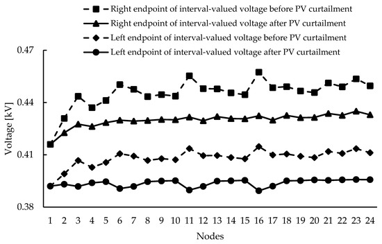
Figure 4. Interval-valued voltages before and after PV curtailment in plan P4.

Plan P5 is obtained by neglecting the correlation among loads and between loads and PVs. The resulting plan is then evaluated under the states of nature that may occur when such correlations exist, as considered in P1–P4. The results are presented in Table 3. The comparison between P5 and P4, conducted using the proposed interval TOPSIS method, indicates that P4 outperforms P5. This result underscores the importance of accounting for correlations among uncertain quantities in fairness improvement planning under uncertainty in low-voltage networks.

It should be noted that (interval) unfairness of PV curtailment is significantly higher in plans P1 and P3 compared to P2, P4, and P5. This result highlights the importance of including PV curtailment unfairness as a criterion, weighted appropriately, in the operational planning of low-voltage networks with high penetration of PVs.

Plans P1–P5 represent solutions obtained by a risk-averse decision maker, using the Hurwicz criterion with $\delta =0$.2 in the ranking process described in Section 3.5. To identify a solution corresponding to a risk-seeking (optimistic) decision maker, Hurwicz criterion with $\delta =0$.8 is applied in the ranking process. This results in plan P6. Notably, the leftmost endpoints of the interval objectives in P6 are lower than those in P4, reflecting the optimistic nature of the decision maker, who weighs more minimal costs (left endpoints) that may occur in a system.

In addition, three fairness improvement plans, P7–P9, are considered to further explore the potential advantages of the proposed approach over other approaches for fairness improvement planning. These plans are derived using the same parameters as plan P4, as shown in Table 2. The results for plans P7–P9 are presented in Table 5.

Table 5. Interval costs and unfairness for plans P7–P9.

Fairness Improvement Plan	P7	P8	P9
Cost of PV curtailment [USD]	[97.2, 98.1]	[93.9, 94.2]	[108.2, 110.2]
Cost of voltage violations [USD]	[8.3, 32.4]	[10.3, 35.1]	[5.4, 24.4]
Unfairness of PV curtailment	[7.4, 12.4]	[6.4, 10.9]	[11.1, 15.2]

Plan P7 is obtained using a combination of uncertain quantities corresponding to their expected values, i.e., crips values obtained from their intervals by using β = 0.5 in Equations (1)–(3). This plan represents a solution that could be obtained using crisp-based (deterministic) approaches, i.e., methods that do not account for uncertainties in input quantities [5,6,7,8]. However, in the presence of uncertainty in the input quantities (loads, PV generation, and slack bus voltage), the result obtained does not represent the optimal fairness improvement plan. Specifically, plan P4 outperforms P7, as the relative closeness to the ideal solution (Equation (29)) for plan P7 is R_P7 = 0.49, which is lower than R_P4 = 0.57. This result highlights the limitations of crip-based (deterministic) approaches in fairness improvement planning under uncertainty.

Plan P8 is obtained by considering the uncertainty in loads and PV generation while neglecting the uncertainty in slack bus voltage. In this case, the value of the slack bus voltage corresponds to the value derived from its interval using β_V = 0.5 in (3). When the uncertainty in the slack bus voltage is considered, plan P8 is no longer the optimal fairness improvement plan. Specifically, plan P4 outperforms P8, as the relative closeness to the ideal solution for P8 is R_P8 = 0.52, which is lower than R_P4 = 0.57. This result shows the potential drawback of approaches that consider uncertainty in loads and PV generation but neglect uncertainty in slack bus voltage, such as the approach proposed in [9].

Plan P9 is obtained by considering the following combination of uncertain quantities: maximum PV generation (PPV_R), minimum load (PD_L), and maximum slack bus voltage (${\mathrm{V}}_{0,\mathrm{R}}$). This combination corresponds to the worst-case scenario, reflecting an extreme operating condition that may occur in the network. Accordingly, P9 represents the solution that could be obtained using robust optimization-based approaches [9,10,11]. However, under uncertainty, this solution is inferior to the one obtained using our approach, as the R_P9 = 0.42 is lower than R_P4 = 0.57. This result demonstrates the potential drawback of robust optimization-based methods in defining the best fairness improvement plan in low-voltage networks under uncertainty. It should also be noted that robust optimization approaches may yield overly conservative solutions [11,14].

In the considered case studies, the PSA algorithm and the TOPSIS calculations were run on a 5.8-GHz processor with 32 GBs of RAM memory. An average solution time of 57.6 s was recorded during the generation of plans P1–P4 and P6. The proposed approach was also tested on a low-voltage network consisting of twice as many demand nodes and PV units as in the original case studies. In this scenario, without utilizing any multiprocessing techniques, the computation time was 192.4 s.

It is important to note that the states of nature are mutually independent, allowing the fairness improvement problems defined by Equations (5)–(18) to be solved independently. This independence enables a significant reduction in overall problem-solving time by executing multiple fairness improvement problems in parallel across different processors or computing units. For example, utilizing multiprocessing techniques on a system with a 16-core processor could potentially reduce the total computation time by up to a factor of 16.

It should be noted that the analyses presented in the paper cannot be performed using the other proposed approaches for fairness improvement planning in low-voltage networks under uncertainty due to the following limitations:

-

They cannot consider a trade-off preference between fairness and costs aligned with the local energy justice policies [19]. This is because most existing approaches treat fairness improvement problem as a single-objective problem rather than a multi-objective one where the objectives differ in dimension. As a result, they are unable to assess trade-off preferences between fairness and costs effectively.

-

They do not consider or evaluate the outcomes (consequences) of a particular solution across different states of nature, i.e., feasible combinations of uncertain quantities (loads, PV generation, and slack bus voltage), defined by the correlations among them, which may occur in an uncertain environment.

-

They cannot account for different decision makers’ risk preferences when evaluating outcomes (consequences) and selecting the best solution.

Note also that the linearization or relaxation of the nonlinear power flow equations, commonly used in the existing approaches, may lead to ineffective fairness improvement plans [11,20].

Furthermore, the approach proposed in this paper provides a comprehensive framework for assessing the hosting capacity in both balanced and unbalanced low-voltage networks under uncertainty, incorporating the decision maker’s risk preferences and the trade-off between fairness and cost. It can also be applied to determine export limits for PV systems, ensuring an optimal balance between curtailment fairness and associated costs across both day ahead and intraday planning horizons.

5. Conclusions

This paper presents a risk-based, multi-objective approach for fairness improvement planning in both balanced and unbalanced low-voltage distribution networks with high PV penetration. The proposed approach accounts for uncertainties in loads, PV generation, and slack bus voltage to identify a solution that minimizes the risk of unfair PV curtailment, as well as the risk of incurring significant costs due to PV curtailment and voltage violations. In finding the optimal solution, the proposed approach addresses the following limitations of the existing methods:

-

Considers trade-off preferences between fairness and costs aligned with local energy justice policies, an aspect not supported by the existing approaches, which treat the fairness improvement problem as a single-objective problem rather than a multi-objective problem with different and conflicting objectives.

-

Evaluates the outcomes of a given solution across feasible combinations of uncertain quantities (states of nature) defined by their correlations.

-

Accounts for different decision makers’ risk preferences when assessing outcomes and selecting the optimal solution.

-

Considers uncertainty in the slack bus voltage.

-

The presented numerical results:

-

Emphasize the importance of addressing fairness improvement planning as a multi-objective problem in low-voltage networks with high PV penetration.

-

Demonstrate the effectiveness of the proposed interval TOPSIS method in capturing diverse decision makers’ risk preferences and trade-off priorities between cost and fairness when selecting the optimal fairness improvement plan.

-

Highlight the significance of considering correlations among uncertain quantities.

The inclusion of energy storage systems and demand response programs as additional resources in fairness improvement planning for PV-rich low-voltage networks is among our future research interests. We also aim to incorporate the fairness of distributed generator curtailment as a criterion in operational planning and optimization for active medium-voltage distribution networks.

Appendix A.1. Hurwicz Criterion

Ranking of intervals $\overline{a}=\left[a_L,a_R\right]$ and$\overline{b}=\left[b_L,b_R\right]$ using the Hurwicz criterion is defined as follows [31,32]:

$$a=\delta ·a_L+\left(1-\delta \right)·a_R, b=\delta ·b_L+\left(1-\delta \right)·b_R$$

(A1)

In (A1), the intervals $\overline{\mathrm{a}}$ and $\overline{\mathrm{b}}$ are mapped to real numbers and then compared. The parameter δ ∈ [0, 1] represents the decision maker’s risk preference. When cost is considered, δ = 1 corresponds to an extremely optimistic decision maker, while δ = 0 corresponds to an extremely pessimistic one. The opposite interpretation applies when benefit is considered. Therefore, by selecting different values of parameter δ in (A1), we can represent more or less optimistic or pessimistic decision makers, i.e., various decision makers’ risk attitudes.

Appendix A.2. An Example of the Advantages of the Proposed Interval TOPSIS Technique

An example discussed in [33] is considered, where a decision maker evaluates three alternatives (plans) (P1, P2, and P3) based on four criteria (F1, F2, F3, and F4), represented as intervals in Table A1. Here, F1 and F2 are benefit criteria, while F3 and F4 are cost criteria. It is assumed that all criteria are equally important, i.e., $w_1=w_2=w_3=w_4=0.25$ in (23). Using the interval extension of the TOPSIS method proposed in [33], the relative closeness to the ideal solution for each alternative is obtained, resulting in the ranking R_P1 > R_P2 > R_P3. Hence, the best plan is P1.

Next, the decision maker applies the proposed interval extension of TOPSIS (21)–(29) to the same problem, again assuming equal importance of criteria, i.e., ${\mathit{w}}_{\mathbf{1}}={\mathit{w}}_{\mathbf{2}}={\mathit{w}}_{\mathbf{3}}={\mathit{w}}_{\mathbf{4}}=\mathbf{0.25}$ in (23).

Table A1. Decision matrix.

	F1	F2	F3	F4
P1	[6, 22]	[10, 15]	[16, 21]	[18, 20]
P2	[15, 18]	[8, 11]	[20, 30]	[19, 28]
P3	[9, 13]	[12, 17]	[42, 48]	[40, 49]

Table A1. Decision matrix.

	F1	F2	F3	F4
P1	[6, 22]	[10, 15]	[16, 21]	[18, 20]
P2	[15, 18]	[8, 11]	[20, 30]	[19, 28]
P3	[9, 13]	[12, 17]	[42, 48]	[40, 49]

First, a risk-seeking (optimistic) decision maker is considered by setting δ = 0.8 for the benefit criteria (F1 and F2) and δ = 0.2 for the cost criteria (F3 and F4). Based on these values, the ranking of intervals in (25) and (26) is performed. In this case, the relative closeness values obtained from (29) are R_P1 = 0.889, R_P2 = 0.719, and R_P3 = 0.661, resulting in the ranking R_P1 > R_P2 > R_P3. Thus, the best alternative is P₁, which matches the solution in [33]. Note that this solution reflects the decision of a risk-seeking decision maker.

Next, a risk-averse (pessimistic) decision maker is considered by setting δ = 0.2 for the benefit criteria and δ = 0.8 for the cost criteria, in order to rank the intervals in (25) and (26). In this case, the obtained values are R_P1 = 0.707, R_P2 = 0.779, and R_P3 = 0.665, leading to the ranking R_P2 > R_P1 > R_P3. Hence, the best alternative is P₂, which differs from the previous case.

It should be emphasized that presented flexibility cannot be achieved using the method proposed in [33], as it does not account for the decision maker’s risk preference in the ranking process. This limitation, which reduces the practical applicability of multi-criteria decision-making methods that do not consider the decision maker’s risk attitudes, is overcome by the proposed interval extension of TOPSIS (21)–(29).

References

- Mai, T.; Nguyen, P.H.; Tran, Q.-T.; Cagnano, A.; De Carne, G.; Amirat, Y.; Le, A.-T.; De Tuglie, E. An overview of grid-edge control with the digital transformation. Electr. Eng. 2021, 103, 1989–2007. [Google Scholar] [CrossRef]
- Fatima, S.; Püvi, V.; Lehtonen, M. Review on the PV hosting capacity in distribution networks. Energies 2020, 13, 4756. [Google Scholar] [CrossRef]
- Dubravac, M.; Fekete, K.; Topić, D.; Barukčić, M. Voltage optimization in PV-rich distribution networks—A review. Appl. Sci. 2022, 12, 12426. [Google Scholar] [CrossRef]
- Tam, T.; Haque, N.A.N.M.M.; Vo, H.T.; Nguyen, H.P. Coordinated active and reactive power control for overvoltage mitigation in physical LV microgrids. J. Eng. 2019, 18, 5007–5011. [Google Scholar] [CrossRef]
- Poudel, S.; Mukherjee, M.; Sadnan, R.; Reiman, A.P. Fairness-aware distributed energy coordination for voltage regulation in power distribution systems. IEEE Trans. Sustain. Energy 2023, 14, 1866–1880. [Google Scholar] [CrossRef]
- Liu, M.Z.; Procopiou, A.T.; Petrou, K.; Ochoa, L.F.; Langstaff, T.; Harding, J.; Theunissen, J. On the fairness of PV curtailment schemes in residential distribution networks. IEEE Trans. Smart Grid 2020, 11, 4502–4512. [Google Scholar] [CrossRef]
- Lusis, P.; Andrew, L.L.H.; Chakraborty, S.; Liebman, A.; Tack, G. Reducing the unfairness of coordinated inverter dispatch in PV-rich distribution networks. In Proceedings of the IEEE Milan PowerTech, Milan, Italy, 23–27 June 2019; pp. 1–6. [Google Scholar] [CrossRef]
- Vadavathi, A.R.; Hoogsteen, G.; Hurink, J. PV inverter-based fair power quality control. IEEE Trans. Smart Grid 2023, 14, 3776–3790. [Google Scholar] [CrossRef]
- Yi, Y.; Verbič, G. Fair operating envelopes under uncertainty using chance constrained optimal power flow. Electr. Power Syst. Res. 2022, 213, 108465. [Google Scholar] [CrossRef]
- Liu, B.; Braslavsky, J.H.; Mahdavi, N. Linear OPF-based robust dynamic operating envelopes with uncertainties in unbalanced distribution networks. J. Mod. Power Syst. Clean Energy 2024, 12, 1320–1326. [Google Scholar] [CrossRef]
- Liu, B.; Braslavsky, J.H. Robust dynamic operating envelopes for DER integration in unbalanced distribution networks. IEEE Trans. Power Syst. 2024, 39, 3921–3936. [Google Scholar] [CrossRef]
- Zhan, S.; Morren, J.; van den Akker, W.; van der Molen, A.; Paterakis, N.G.; Slootweg, J.G. Fairness-incorporated online feedback optimization for real-time distribution grid management. IEEE Trans. Smart Grid 2024, 15, 1792–1806. [Google Scholar] [CrossRef]
- Popovic, Z.; Kovacki, N.; Obrenic, M.; Brbaklic, B. Hosting capacity improvement in low voltage distribution networks: A risk-based approach. In Proceedings of the 27th International Conference on Electricity Distribution (CIRED 2023), Rome, Italy, 12–15 June 2023; pp. 1–5. [Google Scholar] [CrossRef]
- Bertsimas, D.; Sim, M. The price of robustness. Oper. Res. 2004, 52, 35–53. [Google Scholar] [CrossRef]
- Torres, P.J.F.; Ekonomou, L.; Karampelas, P. The correlation between renewable generation and electricity demand: A case study of Portugal. In Electricity Distribution, 1st ed.; Ekonomou, L., Karampelas, P., Eds.; Springer: Berlin, Germany, 2016; pp. 119–151. [Google Scholar]
- Billinton, R.; Li, W. Reliability Assessment of Electric Power Systems Using Monte Carlo Methods; Springer: New York, NY, USA, 1994; pp. 169–179. [Google Scholar]
- Popovic, Z.N.; Knezevic, S.D.; Brbaklic, B. A risk management procedure for island partitioning of automated radial distribution networks with distributed generators. IEEE Trans. Power Syst. 2020, 35, 3895–3905. [Google Scholar] [CrossRef]
- Lan, T.; Kao, D.; Chiang, M.; Sabharwal, A. An axiomatic theory of fairness in network resource allocation. In Proceedings of the IEEE INFOCOM, San Diego, CA, USA, 14–19 March 2010; pp. 1–9. [Google Scholar] [CrossRef]
- Noorman, M.; Apraez, B.E.; Lavrijssen, S. AI and energy justice. Energies 2023, 16, 2110. [Google Scholar] [CrossRef]
- Moring, H.; Mathieu, J.L. Inexactness of second order cone relaxations for calculating operating envelopes. In Proceedings of the IEEE International Conference on Communications, Control, and Computing Technologies for Smart Grids (SmartGridComm), Glasgow, UK, 9–11 October 2023; pp. 1–6. [Google Scholar] [CrossRef]
- Piegat, A.; Landowski, M. Is an interval the right result of arithmetic operations on intervals? Int. J. Appl. Math. Comput. Sci. 2017, 27, 575–590. [Google Scholar] [CrossRef]
- Li, Y.; Zio, E. Uncertainty analysis of the adequacy assessment model of a distributed generation system. Renew. Energy 2012, 41, 235–244. [Google Scholar] [CrossRef]
- Schmidt, M.; Schegner, P. Deriving power uncertainty intervals for low voltage grid state estimation using affine arithmetic. Electr. Power Syst. Res. 2020, 189, 106703. [Google Scholar] [CrossRef]
- Ferson, S.; Kreinovich, V. Modeling correlation and dependence among intervals. In Proceedings of the International Workshop on Reliable Engineering Computing, Savannah, GA, USA, 8–10 February 2006; pp. 115–126. [Google Scholar]
- Vaccaro, A.; Cañizares, C.; Villacci, D. An affine arithmetic-based methodology for reliable power flow analysis in the presence of data uncertainty. IEEE Trans. Power Syst. 2010, 25, 624–632. [Google Scholar] [CrossRef]
- Wang, S.; Dong, Y.; Wu, L.; Yan, B. Interval overvoltage risk based PV hosting capacity evaluation considering PV and load uncertainties. IEEE Trans. Smart Grid 2020, 11, 2709–2721. [Google Scholar] [CrossRef]
- Vidović, P.M.; Sarić, A.T. A novel correlated intervals-based algorithm for distribution power flow calculation. Int. J. Electr. Power Energy Syst. 2017, 90, 245–255. [Google Scholar] [CrossRef]
- Papaefthymiou, G.; Kurowicka, D. Using copulas for modeling stochastic dependence in power system uncertainty analysis. IEEE Trans. Power Syst. 2009, 24, 40–49. [Google Scholar] [CrossRef]
- Czyzak, P.; Jaszkiewicz, A. Pareto simulated annealing—A metaheuristic technique for multiple-objective combinatorial optimization. J. Multi-Criteria Decis. Anal. 1998, 7, 34–47. [Google Scholar] [CrossRef]
- Kamh, M.; Iravani, R. Unbalanced model and power-flow analysis of microgrids and active distribution systems. IEEE Trans. Power Deliv. 2010, 25, 2851–2858. [Google Scholar] [CrossRef]
- Saade, J.J.; Schwarzlander, H. Ordering fuzzy sets over the real line: An approach based on decision making under uncertainty. Fuzzy Sets Syst. 1992, 50, 237–246. [Google Scholar] [CrossRef]
- Popovic, Z.N.; Knezevic, S.D. Dynamic reconfiguration of distribution networks considering hosting capacity: A risk-based approach. IEEE Trans. Power Syst. 2023, 38, 3440–3450. [Google Scholar] [CrossRef]
- Dymova, L.; Sevastjanov, P.; Tikhonenko, A. A direct interval extension of TOPSIS method. Expert Syst. Appl. 2013, 40, 4841–4847. [Google Scholar] [CrossRef]
- Jahanshahlo, G.R.; Hosseinzade, L.F.; Izadikhah, M. An algorithmic method to extend TOPSIS for decision making problems with interval data. Appl. Math. Comput. 2006, 175, 1375–1384. [Google Scholar] [CrossRef]
- Jahanshahloo, G.R.; Hosseinzadeh, L.F.; Davoodi, A.R. Extension of TOPSIS for decision-making problems with interval data: Interval efficiency. Math. Comput. Model. 2009, 49, 1137–1142. [Google Scholar] [CrossRef]
- Ye, F.; Li, Y.N. Group multi-attribute decision model to partner selection in the formation of virtual enterprise under incomplete information. Expert Syst. Appl. 2009, 36, 9350–9357. [Google Scholar] [CrossRef]
- Popovic, Z.N.; Krsman, V.D.; Rakic, M.P.; Airiman, M.E. A risk-based multi-criteria maintenance planning of distribution feeders. Int. J. Electr. Power Energy Syst. 2025, 165, 110379. [Google Scholar] [CrossRef]
- Haque, A.N.M.M.; Nguyen, P.H.; Vo, T.H.; Bliek, F.W. Agent-based unified approach for thermal and voltage constraint management in LV distribution network. Electr. Power Syst. Res. 2017, 143, 462–473. [Google Scholar] [CrossRef]
- Raffi, S.; Rajagopal, R. A scaling law for short term load forecasting on varying levels of aggregation. Int. J. Electr. Power Energy Syst. 2018, 98, 350–361. [Google Scholar] [CrossRef]
- Antonanzas, J.; Osorio, N.; Escobar, R.; Urraca, R.; Martinez-de-Pison, F.J.; Antonanzas-Torres, F. Review of photovoltaic power forecasting. Sol. Energy 2016, 136, 78–111. [Google Scholar] [CrossRef]
Disclaimer/Publisher’s Note: The statements, opinions and data contained in all publications are solely those of the individual author(s) and contributor(s) and not of MDPI and/or the editor(s). MDPI and/or the editor(s) disclaim responsibility for any injury to people or property resulting from any ideas, methods, instructions or products referred to in the content. |
© 2025 by the authors. Licensee MDPI, Basel, Switzerland. This article is an open access article distributed under the terms and conditions of the Creative Commons Attribution (CC BY) license (https://creativecommons.org/licenses/by/4.0/).