Enhanced Adaptive Wiener Filtering for Frequency-Varying Noise with Convolutional Neural Network-Based Feature Extraction ^†

Abstract

Denoising has long been a challenge in image processing. Noise appears in various forms, such as additive white Gaussian noise (AWGN) and Poisson noise across different frequencies. This study aims to denoise images without prior knowledge of the noise distribution. First, we estimate the noise power in the frequency domain to approximate the local signal-to-noise ratio (SNR) and guide an adaptive Wiener filter. The initial denoised result is obtained by assembling the locally filtered patches. However, since the Wiener filter is a low-pass filter, it can remove fine details along with the noise. To overcome this limitation, we post-process the noise and interpolate it between the denoised and original noisy patches to enhance the denoised image. We also mask the frequency domain to avoid grid-like artifacts. Additionally, we introduce a convolutional neural network-based refinement technique to the spatial domain to recover latent textures lost during denoising. The method presents the effectiveness of masking and feature extraction.

1. Introduction

The ultimate goal of the mathematical model for image denoising [1,2,3,4,5,6] is to recover the original image $x\left[m,n\right]$ based on the observed noisy image $B\left[m,n\right]$, as in (1), or based on some learning models [7].

$$B\left[m,n\right]=x\left[m,n\right]+N\left[m,n\right]$$

(1)

First, we provide a brief review of the adaptive Wiener filter [8,9], with the corresponding flowchart (Figure 1). The method can be roughly divided into three stages.

Figure 1. Flowchart of original adaptive Wiener filter.

The first stage is “smoother patch determination”, where relatively smoother patch gradients are collected and transformed to the frequency domain using the fast Fourier transform (FFT). In the second stage, the Fourier-transformed patch gradients are regarded as noise power in the frequency domain. The estimated noise $E\left[p,q\right]$ is obtained by weighting these patches, a process known as sparse band determination. In the final stage, a 2D first-order function $N_{est}\left[p,q\right]$ is used to approximate $E\left[p,q\right]$. With $N_{est}\left[p,q\right]$, the frequency-varying adaptive Wiener filter can be determined for all patches in the noisy image.

However, since the Wiener filter is a signal-to-noise ratio (SNR)-based low-pass filter, it removes texture and details that have less power than the estimated noise. Figure 2, Figure 3, Figure 4 and Figure 5 illustrate the possible drawbacks of the method in Ref. [9]. For denoised patches, the number of nonzero components in a $9\times 9$ FFT is typically less than 10, regardless of patch variance, whereas for sharp image patches, the number of nonzero components exceeds 40. Additionally, since the adaptive filter makes several components equal zero, the resulting patches can exhibit grid-like noise. Therefore, we address these problems and refine the details removed by the adaptive Wiener filter in this study.

Figure 2. Grid-like effect. The left subfigure is the output of patch smoothing from the method in [9] and the right one is the result after masking.

Figure 3. A limitation of the adaptive Wiener filter. The red box indicates the gap between the distributions of filtered patches and sharp patches.

Figure 4. The flowchart of the proposed algorithm. The red circle indicates the post-processing methods of adaptive filtering and detail refinement.

Figure 5. Interpolation mask $M_I$. A warm color indicates a larger value.

2. Proposed Algorithm

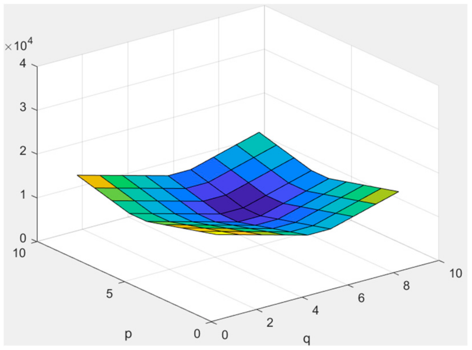
2.1. Adaptive Masking in Frequency Domain

In this phase, features are recovered by interpolating the result with the noisy patch [9]. The interpolation ratio is determined as

$${\mathrm{P}}_{new}=\left(M_I\right)·{\mathrm{P}}_{denoised}+\left(1-M_I\right)·{\mathrm{P}}_{noisy}$$

(2)

where $M_I=e^{-{\displaystyle \frac{idx}{81}}}$.

We specify the top-left coordinate of a patch $\left(p_1, q_1\right)$ as (1,1), with $q_i$ increasing from left to right and $p_i$ increasing from top to bottom. The parameter $\mathrm{idx}$ in (1) is calculated as $\mathrm{idx}=p_i·q_i$. The Wiener-filtered patch takes a larger proportion in the low-frequency component. In other words, we preserve information in the high-frequency components from the noisy patch. After the interpolation, we apply an overall mask $M_O$ to the new patch ${\mathrm{P}}_{new}$. Ideally, ${\mathrm{P}}_{new}$ is smoothed in the low-variance area, and its details are preserved in the high-variance area. However, when dealing with noisy image patches, the variance deviates from the true variance. Therefore, we use the number of nonzero coefficients in the Wiener filter $H\left[p,q,a,b\right]$ [9] as a lookup parameter, denoted as $nz$. Here $p,q$ are indices in the frequency domain, while $a,b$ represent the spatial location of current patch $\mathrm{P}$ in the noisy image. When the number of nonzero components is small, we classify the patch as a smooth area, and most high-frequency components are forced to zero by $M_O$ (3). Conversely, if the Wiener filter $H$ has few zero components, the filter performs well, making $M_O$ an all-pass filter (Figure 6, Figure 7 and Figure 8).

$${\mathrm{P}}_{out}=M_O·{\mathrm{P}}_{new} \mathrm{where} M_O=e^{-{\displaystyle \frac{{\mathrm{idx}}^2}{n{z}^3}}}$$

(3)

Figure 6. CNN architecture of detail refinement.

Figure 7. $M_O$ coefficient of $nz$ number (left) $2$, (middle) $10$, and (right) $70$. A warm color indicates a larger value.

Figure 8. Training for detail refinement.

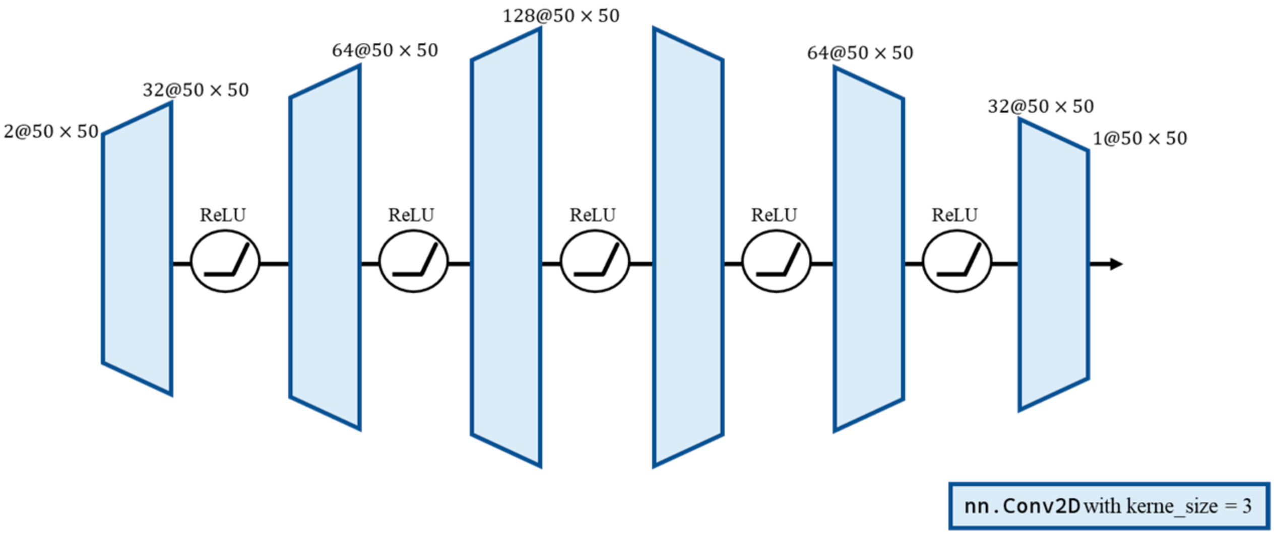
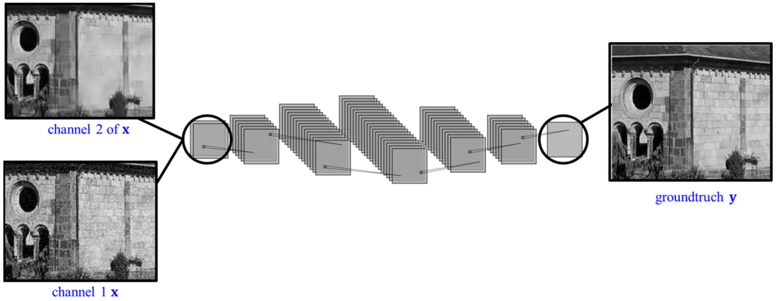
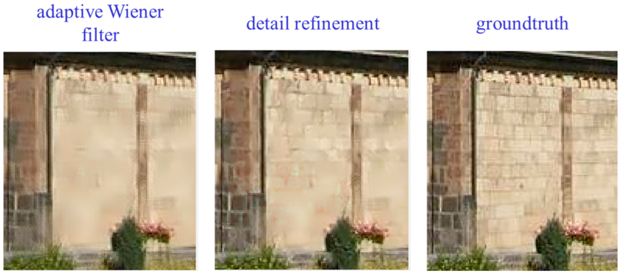
2.2. Detail Refinement

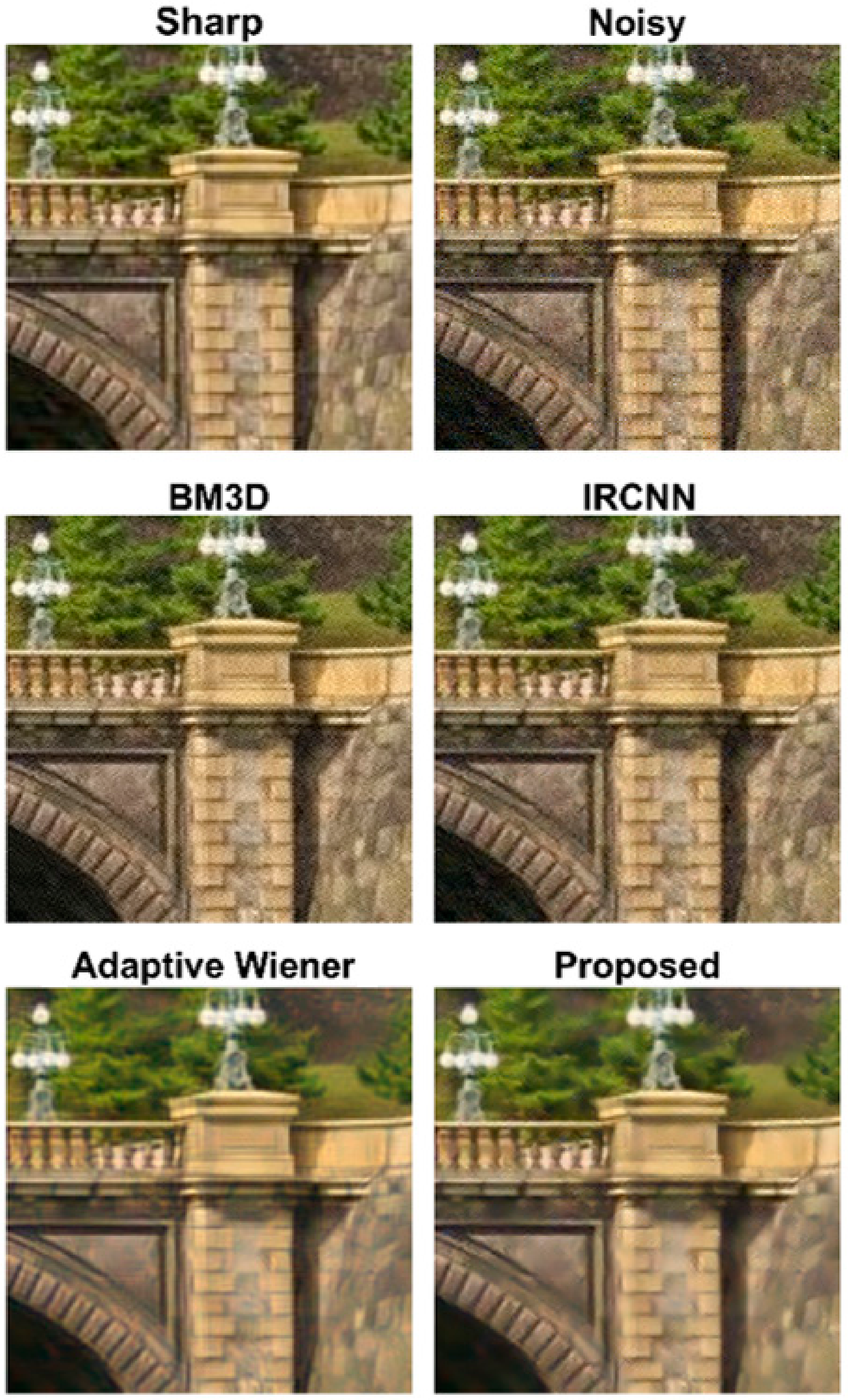
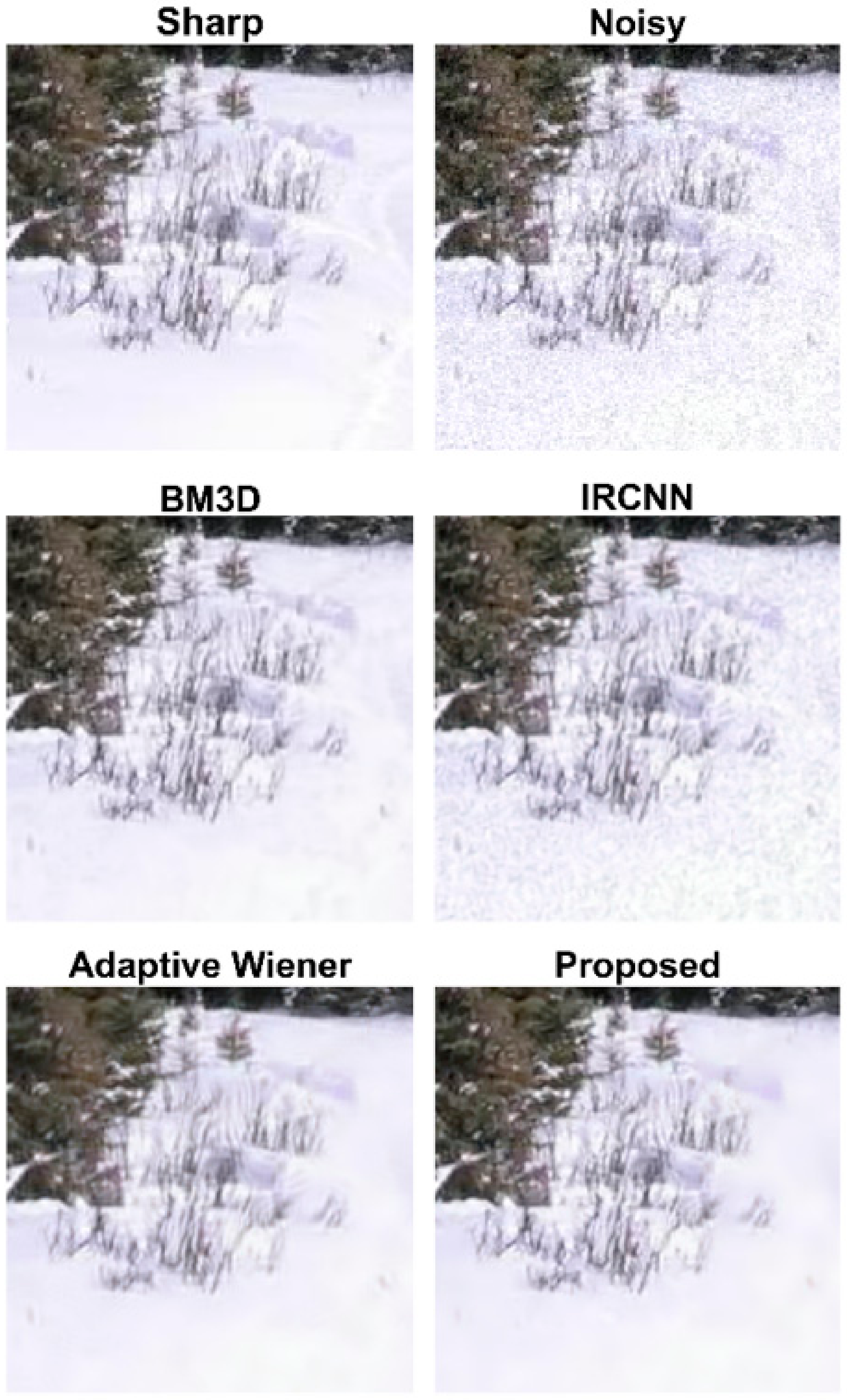
After recovering high-frequency components via masking in the Fourier domain, the remaining challenge is preserving fine patch details spatially. For instance, in the case of a brick wall, the gaps between bricks cannot be captured by masking alone. These details are inherently spatial. Therefore, we aim to extract subtle features by training a convolutional neural network (CNN) based on the following architecture.

The CNN model takes a $50\times 50\times 2$ input, with the target being a $50\times 50\times 2$ patch. The first channel of the input is the noisy image patch, and the second channel is the result of the adaptive Wiener filter. We train the combination against the true image patch. In training, we use MSE as the loss function (4).

$$l_n={\displaystyle \frac{1}{N}}{\displaystyle \sum }_{i=1}^N{\left(f_{\theta }\left({\mathrm{x}}_{\mathrm{i}}\right)-y_i\right)}^2$$

(4)

The ground truths of the training data are collected from ImageNet-A dataset [7]. For each image $Y_i$, we apply AWGN with a standard deviation uniformly sampled in the range of [0, 30]. After applying the proposed blind denoising, we randomly select patches to form $x_i$ and the corresponding patch in $Y_i$ is ${\mathrm{y}}_{\mathrm{i}}$. The idea here is to consider both the MMSE-denoised result—i.e., the adaptive Wiener filter—and the original noisy image patch with possible latent details. This model extracts spatial features from both the Wiener-filtered result and the original noisy image patch (Figure 9).

Figure 9. A visualization of the effect of detail refinement.

3. Results

We assessed the performance of the developed model in this study in four different scenarios: AWGN, Poisson noise, and two frequency-varying noise distributions. We compared the results with those obtained using IRCNN [6], BM3D, and the adaptive Wiener filter. For a restored image $y\left[m,n\right]$ and its corresponding ground truth $x\left[m,n\right]$, the performance metric used was peak SNR (PSNR) (5).

$$PSNR=10 {\mathit{log}}_{10}{\displaystyle \frac{{255}^2}{\frac{1}{MN}{{\displaystyle \sum }}_{m=1}^M{{\displaystyle \sum }}_{n=1}^N{\left|y\left[m,n\right]-x\left[m,n\right]\right|}^2}}$$

(5)

The test set comprises five real-world images. For each scenario, we present the estimated noise spectrum and enlarged views of the results.

3.1. AWGN

The noise $N\left[m,n\right]$ is normally distributed with a mean of 0 and a standard deviation of 15, which is represented as

$$N\left[m,n\right] ~ \mathcal{N}\left(0, {15}^2\right)$$

(6)

The noise distribution for the model as in (6) is plotted as in Figure 10. Then, in Table 1, the restoration performance for the image degraded by the noise in (6) is shown. Some visual reconstruction results are shown in Figure 11.

Figure 10. $N_{est}\left[p,q\right]$ for AWGN. A warm color means a larger value.

Table 1. The restoration performance of images degraded by the noise model in (6).

PSNR	Castle	Pillar	Bridge	Cottage	Snow Field	Average
Adaptive Wiener [9]	29.273	31.703	29.886	30.639	28.766	29.273
BM3D [5]	27.010	28.704	27.200	27.714	27.003	27.010
IRCNN [6]	26.799	27.874	27.059	27.255	27.048	26.799
Proposed	30.310	31.965	30.640	30.981	29.381	30.310

Figure 11. Enlarged visualization of restoration for AWGN.

3.2. Poisson Noise

When the noise follows a Poisson distribution, (7) is used.

$$N\left[m,n\right] ~ Poisson\left(x\left[m,n\right]\right)$$

(7)

The distribution of the Poisson noise in (7) is shown in Figure 12. The restoration performance for the images degraded by the noise in (7) is shown in Table 2 and Figure 13 show some visual results of image restoration.

Figure 12. $N_{est}\left[p,q\right]$ for Poisson noise. A warm color means a larger value.

Table 2. The restoration performance of images degraded by the noise model in (7).

PSNR	Castle	Pillar	Bridge	Cottage	Snow Field	Average
Adaptive Wiener [9]	32.889	34.548	32.658	32.286	31.662	32.809
BM3D [5]	32.665	35.108	32.709	32.684	32.142	33.062
IRCNN [6]	31.866	34.436	32.055	32.227	31.524	32.421
Proposed	33.095	35.095	33.154	32.910	32.099	33.271

Figure 13. Enlarged visualization of restoration for Poisson noise.

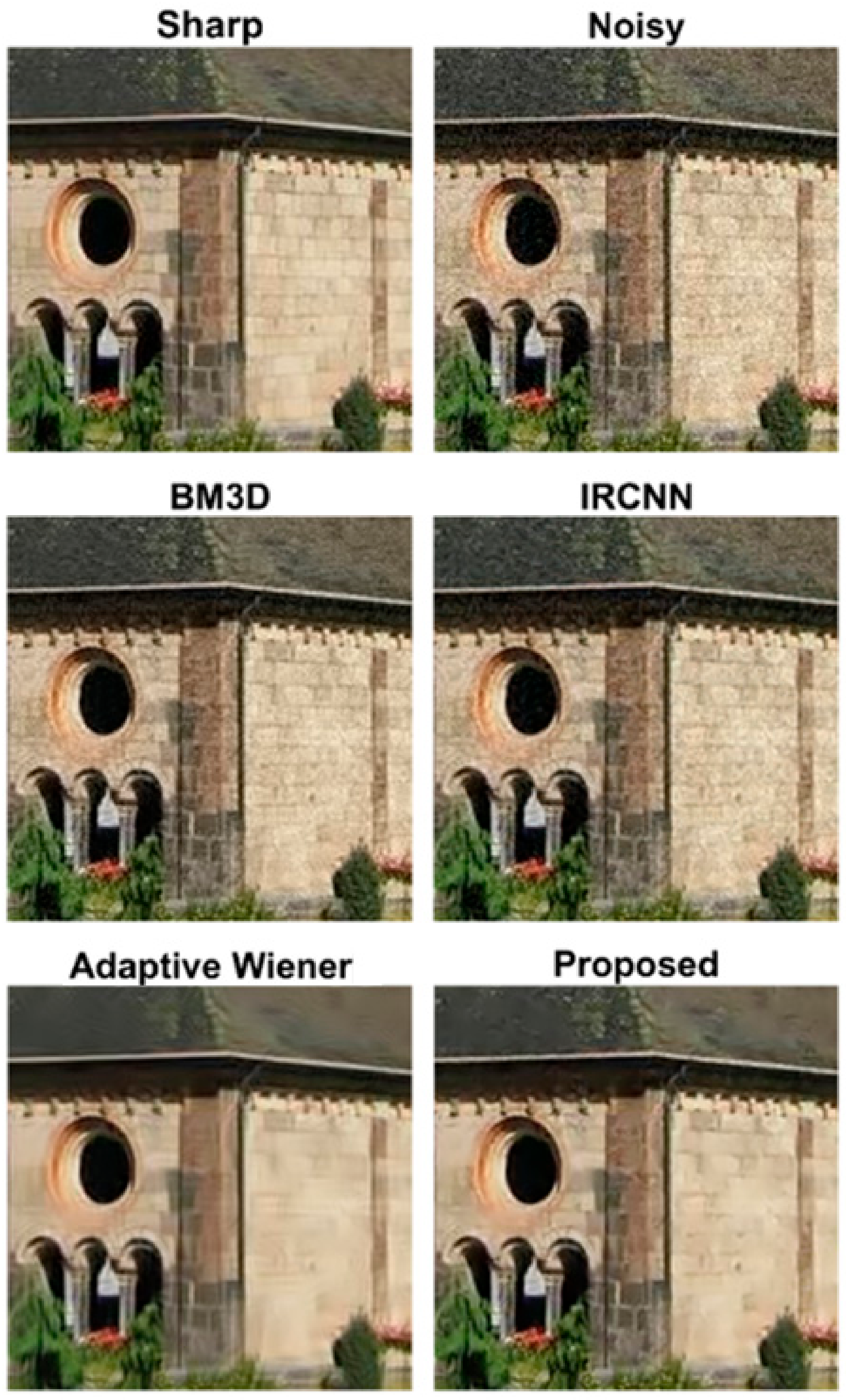
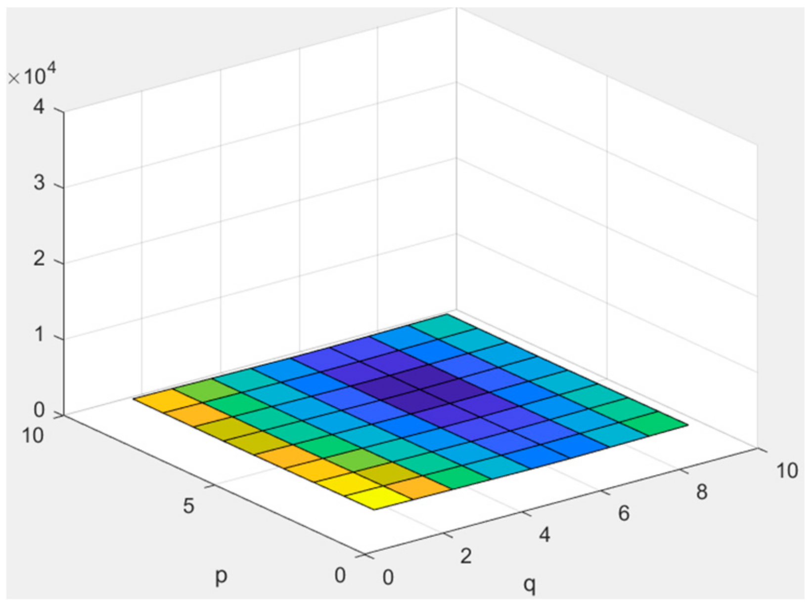
3.3. Frequency-Varying Noise (Peak-like)

Given the noise spectrum of AWGN in Section A, denoted as $N_0/2$, we apply a peak-like frequency-varying noise characterized by

$$E\left(N\left[p,q\right]\right)=N_0({\displaystyle \frac{p_1}{M}}+{\displaystyle \frac{q_1}{N}})$$

(8)

where the $M$ and $N$ denote the height and width of the image, and $N\left[p,q\right]$ represents the $M\times N$ point FFT of the AWGN. The indices are symmetric, with p₁ = min(p, M−p), and q₁ = min(q, N−q). The noise model in (8) is plotted in Figure 14. The restoration performance for the images interfered by the noise in (8) is shown as in Table 3. In Figure 15, some visual results of the reconstructed images are shown.

Figure 14. $N_{est}\left[p,q\right]$ for (8). A warm color means a larger value.

Table 3. The restoration performance of images degraded by the noise model in (8).

PSNR	Castle	Pillar	Bridge	Cottage	Snow Field	Average
Adaptive Wiener [9]	27.778	29.176	28.491	28.415	27.278	28.227
BM3D [5]	21.519	22.807	21.839	21.965	21.990	22.024
IRCNN [6]	23.927	24.841	24.251	24.323	24.260	24.321
Proposed	28.637	28.900	28.816	28.181	26.888	28.285

Figure 15. Enlarged visualization of restoration for peak-like frequency varying noise.

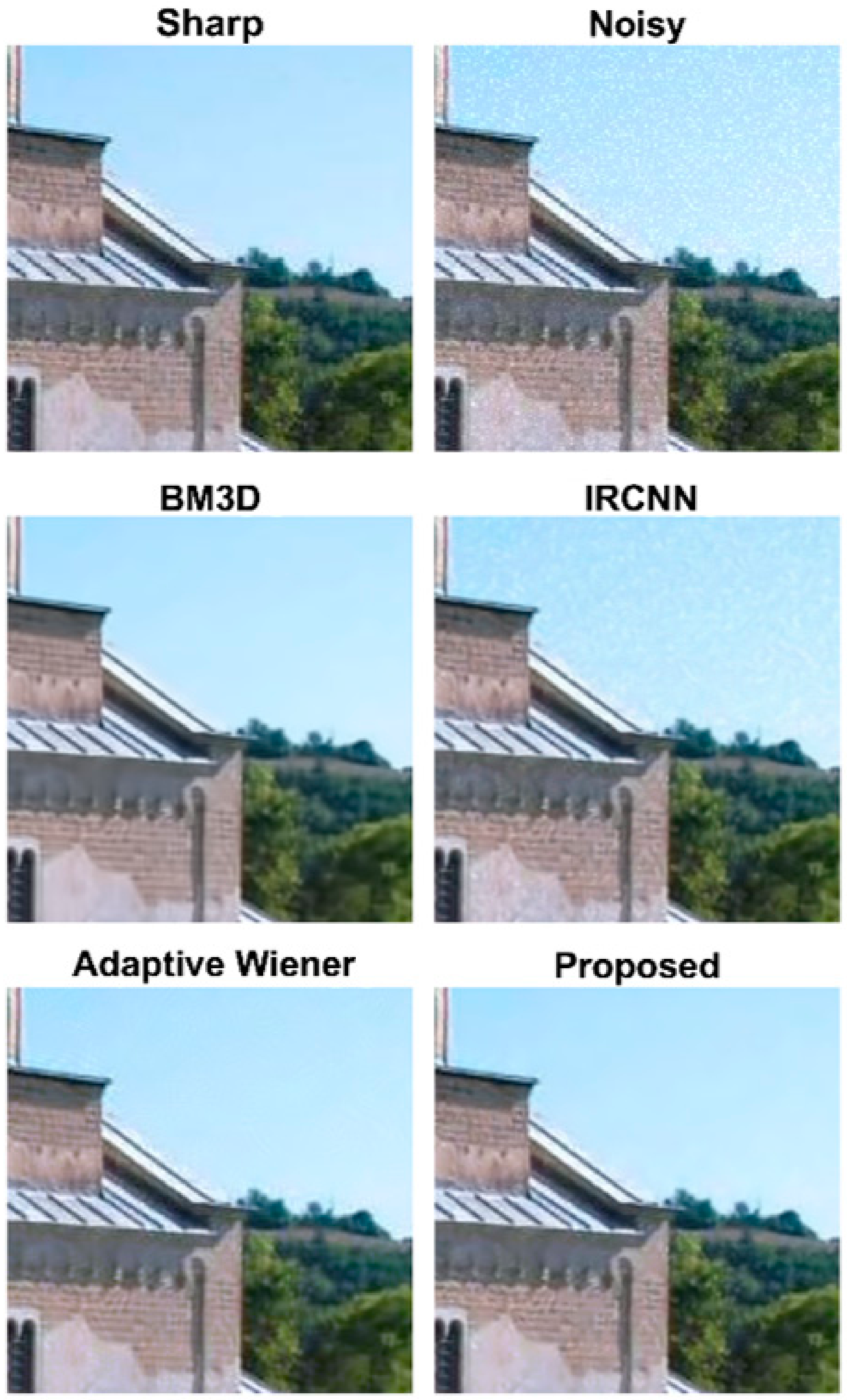
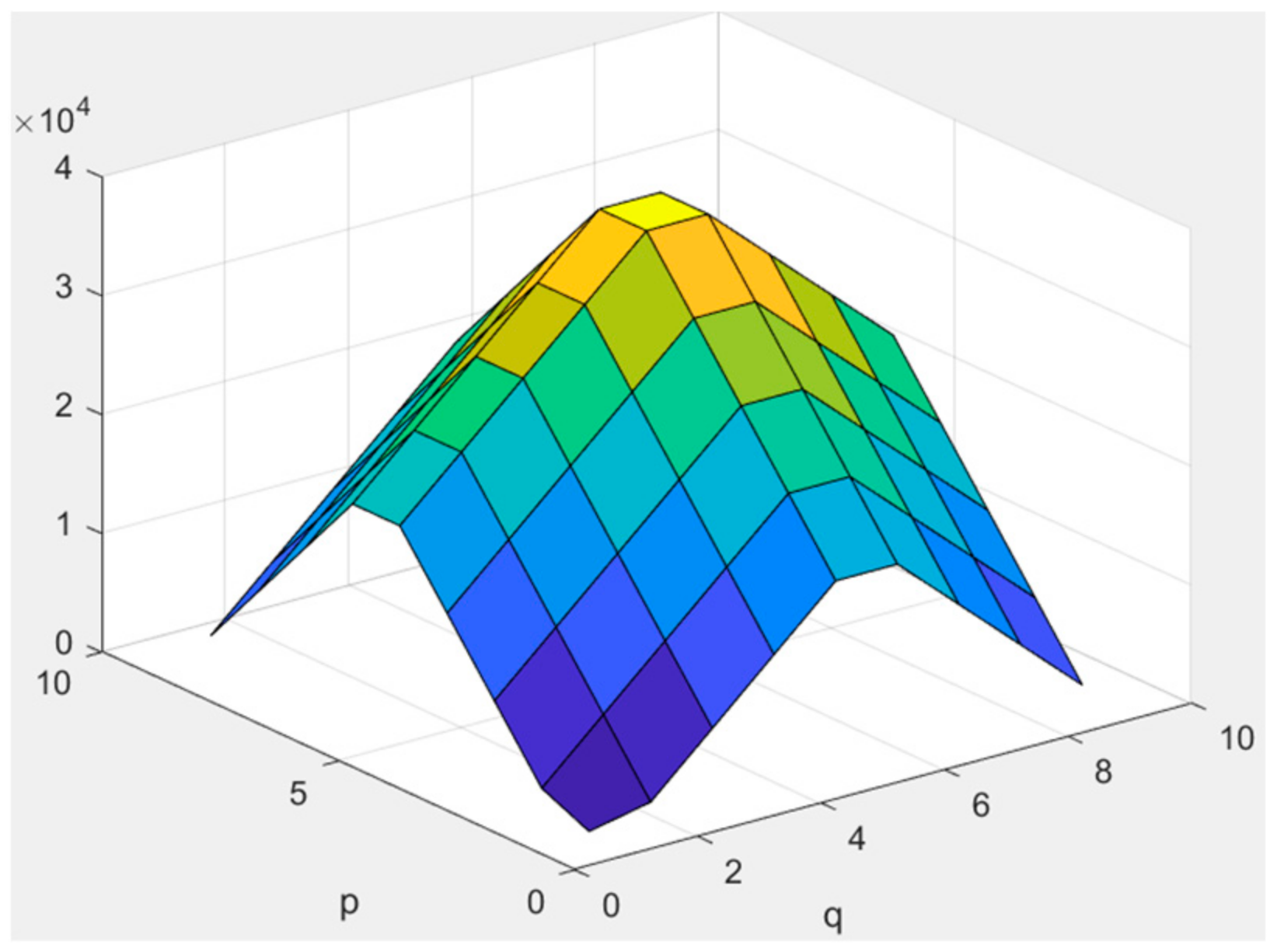
3.4. Frequency-Varying (Valley-like) Noise

Using the same notation as in Section C, the noise distribution exhibits a valley-like surface in the frequency domain, described by:

$$E\left(N\left[p,q\right]\right)=N_0(1-{\displaystyle \frac{0.4·p_1}{M}}-{\displaystyle \frac{0.4·q_1}{N}})$$

(9)

The noise model in (9) is plotted in Figure 16. The restoration performance for the images interfered by the noise in (9) is shown as in Table 4. In Figure 17, some visual results of the reconstructed images are shown.

Figure 16. $N_{est}\left[p,q\right]$ for (9). A warm color means a larger value.

Table 4. The restoration performance of images degraded by the noise model in (9).

PSNR	Castle	Pillar	Bridge	Cottage	Snow Field	Average
Adaptive Wiener [9]	31.338	33.561	31.488	32.293	30.644	31.865
BM3D [5]	31.865	33.612	31.961	32.594	31.104	32.227
IRCNN [6]	30.051	31.097	30.328	30.575	30.075	30.425
Proposed	32.032	33.513	32.068	32.498	31.215	32.265

Figure 17. Enlarged visualization of restoration for valley-like frequency-varying noise.

3.5. Average Runtime per Image

Taking the image ‘Castle’ as an example, with a size of $1006\times 782\times 3$, BM3D [5] takes 47 s to restore the image, while IRCNN [6] takes only 2 s, and the adaptive Wiener filter [9] requires 5 s. The proposed postprocessing takes 15 s.

4. Conclusions

In this study, we improved the adaptive Wiener filter [9]. For the original adaptive Wiener filter, a noise-free image must be sparse in some space-frequency domain for the determination of the noise distribution based on smooth patches. The noise model is then derived from this distribution, enabling the automatic design of an adaptive Wiener filter for frequency-varying noise spectra. However, the original adaptive Wiener filter tends to erase most of the details in the denoised image and may introduce grid-like noise. To address these issues, we interpolated the filtered result with the original patch to recover a certain amount of high-frequency components. After interpolation, a mask was applied to remove the blocking effect. To further enhance performance, we trained a CNN to retrieve the details lost during filtering. This method represents a trade-off between processing time and performance. Although the proposed detail refinement CNN was specifically trained to extract features under AWGN conditions, the developed method demonstrates the best average performance under Poisson noise and frequency-varying noise when compared to other approaches. The method effectively processes various noise distributions and achieves these results within a reasonable time frame.

References

1. Lebrun, M. An analysis and implementation of the BM3D image denoising method. Image Process. Line 2012, 2, 175–213. [Google Scholar] [CrossRef]
2. Pyatykh, S.; Hesser, J.; Zheng, L. Image noise level estimation by principal component analysis. IEEE Trans. Image Process. 2012, 22, 687–699. [Google Scholar] [CrossRef] [PubMed]
3. Liu, X.; Tanaka, M.; Okutomi, M. Single-image noise level estimation for blind denoising. IEEE Trans. Image Process. 2013, 22, 5226–5237. [Google Scholar] [CrossRef]
4. Ding, J.J.; Chang, J.Y.; Liao, C.L.; Tsai, Z.H. Image deblurring using local Gaussian models based on noise and edge distribution estimation. In Proceedings of the TENCON 2021—2021 IEEE Region 10 Conference, Auckland, New Zealand, 7–10 December 2021; pp. 714–719. [Google Scholar]
5. Dabov, K.; Foi, A.; Katkovnik, V.; Egiazarian, K. Image denoising by sparse 3-d transform-domain collaborative filtering. IEEE Trans. Image Process. 2007, 16, 2080–2095. [Google Scholar] [CrossRef] [PubMed]
6. Zhang, K.; Zuo, W.; Gu, S.; Zhang, L. Learning deep CNN denoiser prior for image restoration. In Proceedings of the IEEE Conference on Computer Vision and Pattern Recognition (CVPR), Honolulu, HI, USA, 21–26 July 2017; pp. 3929–3938. [Google Scholar]
7. Hendrycks, D.; Zhao, K.; Basart, S.; Steinhardt, J.; Song, D. Natural adversarial examples. In Proceedings of the IEEE/CVT Conf. Computer Vision and Pattern Recognition, Nashville, TN, USA, 19–25 June 2021; pp. 15262–15271. [Google Scholar]
8. Zhang, X. Image denoising using local Wiener filter and its method noise. Optik 2016, 127, 6821–6828. [Google Scholar] [CrossRef]
9. Ding, J.J.; Liao, C.L. Image denoising based on the noise prediction model using smooth patch and sparse domain priors. In Proceedings of the International Workshop on Advanced Imaging Technology (IWAIT), Jeju, Republic of Korea, 9–11 January 2023; Volume 12592, pp. 170–175. [Google Scholar]
Disclaimer/Publisher’s Note: The statements, opinions and data contained in all publications are solely those of the individual author(s) and contributor(s) and not of MDPI and/or the editor(s). MDPI and/or the editor(s) disclaim responsibility for any injury to people or property resulting from any ideas, methods, instructions or products referred to in the content.
Article Metrics
Citations
Article Access Statistics
Multiple requests from the same IP address are counted as one view.