Abstract
Dilution of Precision (DOP) is routinely used in GNSS to assess the quality of the constellation geometry for the positioning algorithm. Those DOP indicators are computed from the estimation covariance of a snapshot weighted least squares (WLS) estimate under certain hypotheses. This paper proposes to define DOP indicators for GNSS solutions based on Factor Graph Optimization (FGO). FGO solutions have become popular in the GNSS domain. They allow to easily model probabilistic contraints, called factors, over a large time window, by mixing observations and motion constraints accross consecutive epochs. The solution is solved by performing a batch WLS estimation for the states at all considered epochs, using all available factors. Due to the simple nature of the estimation algorithm—a WLS solution—it is possible to derive the theoretical estimation error covariance, which will indicate the accuracy of the computed solution. In this paper, a formula is proposed to approximate the DOP for the FGO solution. Then, the formula is validated in various scenarios involving fixed or changing satellite visibility.
1. Introduction
The positioning algorithms implemented in GNSS receivers uses estimation techniques to combine GNSS observations, such as code pseudo-ranges or doppler offset measurements, to estimate the unknown position, velocity and clock bias of a GNSS receiver. Several algorithms are commonly used, such as the Weighted Least Squares estimation and the Kalman Filter [1,2]. The Weighted Least Squares (WLS) estimation applied with code pseudo-ranges is called the Single Point Positioning (SPP) solution, and is the most basic solution provided by a GNSS receiver. Kalman filter-based techniques add a state transition model, which corresponds to a motion model for the position/velocity/clock states, in order to refine the estimate [3]. It can also be applied with phase pseudo-range observations, leading the well-known Precise Point Positioning [4].
Those algorithms provide both the estimate and the covariance matrix of the state vector. The covariance matrix gives an indication of the uncertainty of the estimate, and its validity depends on the matching of the assumed models with the real conditions of the data collect. Among the usual quality indicators, the DOP (Dilution of Precision) factors are often encountered [1]. The DOP indicators are derived from the estimation covariance of the WLS solution, assuming that all code pseudo-ranges are affected by a Gaussian error that has the same variance and is independent from other pseudo-ranges. Given those assumptions, the DOP indicators only depend on the relative satellite positions with regards to the receiver. They quantify the impact of the satellite constellation geometry on the uncertainty of the WLS solution. In the context of this paper, satellite constellation geometry refers both to the satellite position relative to the receiver, but also to the possible masking of satellites by surrounding obstacles. DOP is used for assessment of solution quality, filtering bad position estimates or planning data collections.
More recently, Factor Graph Optimization (FGO) has been applied to the GNSS positioning problem with great success [5,6]. FGO performs a batch WLS estimation over a large time window, as opposed to a snapshot algorithm as used in the SPP solution. In order to benefit from the optimization over a large time window, motion factors are introduced in addition to GNSS observations to provide constraints between states in adjacent epochs. Those motion factors are essentially similar to the state transition model in a Kalman filter. Therefore, all observations contribute to the accuracy of the solution at each epoch, through the correlation of the estimated states across epochs introduced by the motion factors.
While the impact of the constellation geometry on the solution accuracy is well described for snapshot WLS solutions, such as the SPP solution, it is more difficult to determine how the constellation geometry will impact the solution accuracy in an FGO solution, due to the intricate interactions between the GNSS observations at each epochs and the propagation of the accuracy through the motion factors.
This paper aims at deriving a DOP-like indicator for FGO solutions including a generic motion factor, that will provide a quality assessment of a FGO solution at each epoch, based on the constellation geometry and motion factor uncertainty only.
2. Materials and Methods
2.1. DOP Indicator in a Snapshot Least Squares Solution
In this section, the considered positioning algorithm is the SPP algorithm, consisting in the estimation of the 3D position and the receiver clock bias from GNSS code observations at a single epoch k. j is used to index the scalar states within the state vector:
The linearized observation model around an approximate position is:
where is observation vector comprising all GNSS code observations at epoch k, is the unknown state vector, is the Jacobian matrix of the code observation model and is the observation error vector, assumed normally-distributed, centered with a covariance .
The WLS estimate of [7], referred to as the snapshot solution is given by Equation (2) and its covariance matrix is given by Equation ():
Assuming that the observation error is independent and identically-distributed accross all available observations, i.e., , we obtain:
where is the standard deviation of the GNSS code observations.
This expression separates the contribution of the measurement noise from the geometry of the constellation. We note the DOP matrix. The different DOP indicators are computed from the diagonal elements of [1]. For example, assuming that the 3D position is placed on the first 3 elements of the state vector :
- Global DOP:
- Position DOP:
where refers to the element at row i and column j of a matrix .
2.2. Factor Graph Model
In this study, a simple factor graph (Figure 1) is considered for one scalar state at different epochs indexed by . refers to one of the scalar state at epoch k, such as the position along one axis or the receiver clock bias.
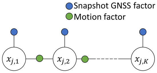
Figure 1.
Factor graph considered in this study.
We assume that the snapshot LS algorithm provides a solution for each of the K epochs of a trajectory. From each snapshot solution, the snapshot estimation accuracy is used as a factor to constrain the scalar state at epoch k and is referred to as snapshot GNSS factor.
An additional factor is introduced to model the probabilistic constraint linking the scalar states at two consecutive epochs. It assumes that the evolution of the scalar state between 2 epochs is known, with an uncertainty assumed to be normally-distributed with a standard deviation q. This constraint is referred to as a motion factor in this document. This generic motion factor uses the following affine model:
where accounts for the uncertainty of the motion constraint, assumed to be a centered normal random variable with a constant standard deviation q and is a known parameter, e.g., an integrated velocity coming from another sensor.
Examples of motion constraints are the estimation of the receiver displacement by GNSS Doppler or Time Difference of Carrier Phase measurements [6], estimation of the receiver displacement by an external sensor such as an inertial measurement unit or a visual simultaneous localization and mapping solution [2], or simply a dynamic model, such as a random walk or constant velocity model with Gaussian uncertainty [3].
Finally, it is assumed that the errors of the snapshot GNSS factors and those of the motion factors are independent between each other and across epochs. Therefore, when stacking all the factors in a single vector , we obtain the following estimation problem:
2.3. Batch Least Squares Solution of the Considered Factor Graph
When ignoring the motion constraints in Equation (7), we find the trivial solution which is called the snapshot solution. For this particular solution, the snapshot covariance matrix for state accross all epochs from 1 to K is:
The solution of the factor graph mixing both snapshot GNSS factors and motion factors is referred to as the batch solution. The batch solution covariance matrix is obtained with the following equation.
The inverse of the batch solution covariance is a so-called a tri-diagonal matrix [8].
2.4. Efficient Computation of the Batch Estimation Covariance
To compute efficiently the batch solution covariance matrix, one can use the particular shape of (10). Additionally, we are interested only in the diagonal elements of the matrix, to characterize the uncertainty of the considered scalar state estimate at each epoch k. The symbolic expression of the diagonal elements for the first few values of K is shown in Appendix A. It is observed that the k-th diagonal element is a ratio of 2 expressions and which depend on :
The denominator is common to all epochs of the considered trajectory. It can be computed using a second-order linear recurrence relation:
The numerator depends on the considered epochs within the trajectory and can be computed using the following expression:
where is the evaluation of expression at and leaving other parameters untouched.
The expressions of and have been validated by comparing the diagonal elements of Equation (10) to the values computed using Equation (11), using a symbolic mathematical software up to , and numerical simulations up to . Elements of the mathematical demonstration to obtain those expressions are available in Appendix B.
2.5. DOP Computation for a Factor Graph Optimization Solution
By definition, e.g., in [1], the DOP indicator is defined as the ratio between the uncertainty of the combined estimated states and the uncertainty of the GNSS observations, assuming that all GNSS observations are independent and affected by an error with the same variance :
where is the estimation variance of state , and is the set of indexes of the scalar states of interest. For example, if the state vector at a particular epoch is composed of , to compute the horizontal DOP, one has to combine the east and north position uncertainty and .
The previous section provided the estimation uncertainty computation for both snapshot and batch solutions, for a scalar element of the state vector. The computation can then be performed for the scalar states of interest before combining them into a DOP indicator.
We define the DOP indicators coming from the snapshot solution, noted , and the one coming from the batch solution including a motion factor, noted
Note that while the snapshot DOP does not depend on , the batch DOP depends on the ratio between the motion uncertainty and the observation uncertainty .
3. Results
3.1. Validation Method of the Proposed Batch DOP Formula
The formula, Equation (11), to obtain uncertainty for a batch solution from the snapshot scalar uncertainty has been validated for a single scalar state.
However, when combining the uncertainty of several scalar states to compute a DOP indicator, the correlated impact of an observation error on the different states should be accounted. This is not the case for the batch DOP computed using Equation (), since the diagonal elements of the covariance matrix of the batch solution are approximated by considering each scalar state uncertainty independently from the other states.
The following subsections aim at quantifying the impact of this approximation. To do so, the batch DOP obtained from Equation () and the exact batch DOP, obtained by computing the covariance of the full state vectors with Equation (10), are compared based on the difference of HDOP and the ratio of HDOP. The results are summarized in Table 1.

Table 1.
HDOP difference and ratio between proposed formula and exact computation.
3.2. Validation the FGO DOP Formula in a Fixed Constellation Case
When considering several consecutive epochs at a high rate (typically higher than 0.1 Hz), the constellation geometry can be considered as fixed over a window of a few tens of epochs. In the case of an open sky receiver, the snapshot DOP will typically remain constant, except when one satellite appear or disappear in the antenna’s field of view.
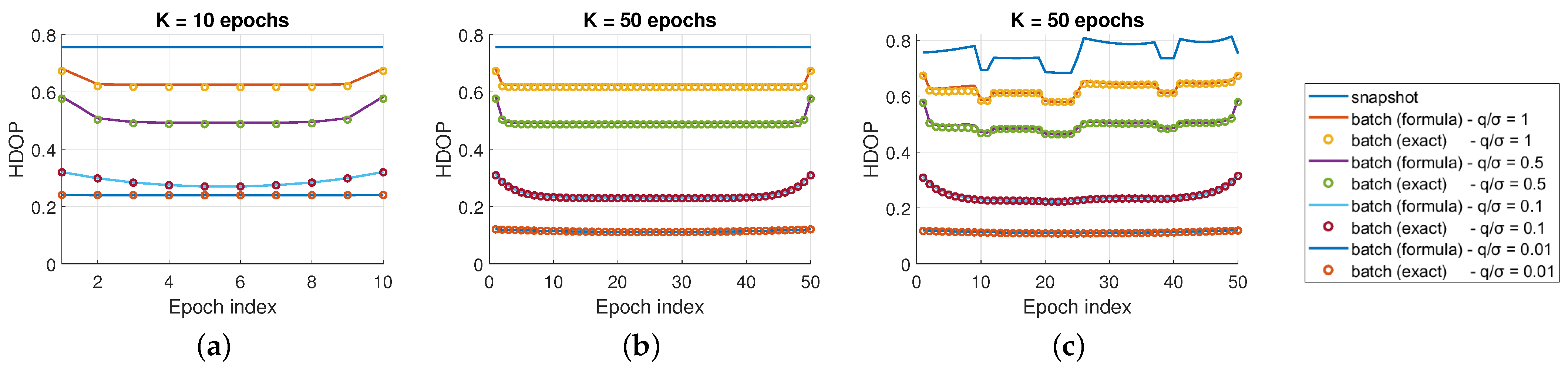
The considered scenario is the nominal GPS constellation from IS-GPS-200M seen by a fixed receiver in Toulouse on the 1st of January 2023 at 00:00. Figure 2a,b shows the batch HDOP for all epochs for a mix of factor graph length K and motion to observation uncertainty ratio . The HDOP value computed with the formula is close to the exact HDOP value, especially for low values of .
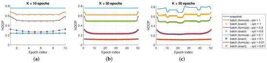
Figure 2.
HDOP comparison for fixed (a,b) and time-varying (c) constellation geometry.
On the general shape of the batch DOP, we can observe that the DOP is lower in the middle of the graph. This is due to the fact that all surrounding epochs contribute to the accuracy at a particular epoch. Secondly, the overall accuracy depends on the value of : the lower is, the better the accuracy is. Finally, for larger , the DOP usually reaches a floor value for the central part of the trajectory that is common for different values of K. This points towards the fact that increasing the factor graph length may not result in better accuracy once the floor has been reached.
3.3. Validation of the FGO DOP Formula in a Varying Constellation Case
In this section, the nominal GPS constellation from IS-GPS-200M is considered. The scenario considers a fixed receiver in Toulouse on the the 1st of January 2023 with a 5-min interval over the first hours of the day. This scenario allows to have varying and realistic constellation geometries, leading to temporal variations of the snapshot DOP.
Figure 2c shows the exact HDOP and the HDOP computed using Equation () for a fixed value of and various values of . Again, the HDOP values obtained with the formula are close to the exact values.
An interesting observation can be made. For high accuracy motion constraints (e.g., ), variations of HDOP are attenuated and the batch HDOP reaches a floor value for central epochs. In this particular cases, the accurate motion constraints allow to have a good relative accuracy between consecutive position estimates, and the observations from every epoch to contribute to the absolute accuracy of the whole trajectory.
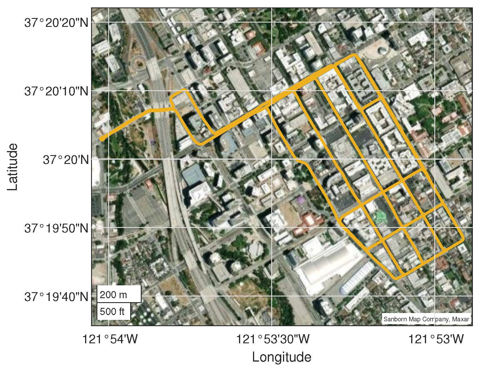
3.4. Validation of the FGO DOP Formula in Constrained Urban Case
In this section, we study the case where the constellation geometry is changing in time due to the masking by building as a GNSS receiver is moving across a city. The considered trajectory comes from the Google Smartphone Decimeter Challenge 2021 [9], and trajectory “2021-04-28-US-SJC-1/Pixel4” has been chosen as it passes through an urban center. Figure 3 shows the 2D trajectory. Frequent satellite masking occur leading to frequent snapshot HDOP degradation.

Figure 3.
Trajectory “2021-04-28-US-SJC-1/Pixel4” from the GSDC2021 dataset.
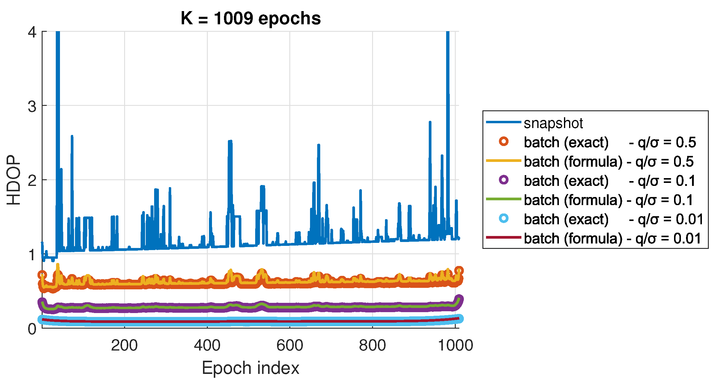
Figure 4 shows the exact HDOP and the HDOP computed using Equation () for , i.e., all available epochs at 0.5 Hz, and various values of . Again, the HDOP values obtained with the formula are close to the exact values. The largest difference corresponds to epochs where fewer satellites are available. At those epochs, sparse GNSS observations results in larger correlation between the east and north position estimation errors, and therefore, larger approximation error of the proposed formula.
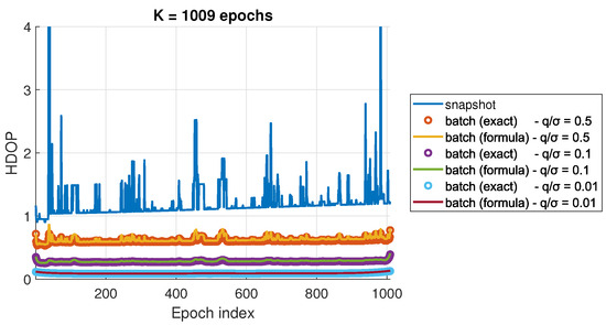
Figure 4.
HDOP comparison for urban masking scenario.
The FGO solution improves the accuracy of the solution, even in the epochs without enough satellites to compute a solution. For those epochs, the snapshot uncertainty has been clipped to a value of 100 m for each position state. Again, the temporal DOP variations are attenuated in the case of highly accurate motion uncertainties.
4. Discussion
This paper proposes a definition of the notion of DOP for batch solution including a generic motion factor, applicable to FGO solutions. The obtained DOP indicator mainly depends on the snapshot DOP, the FG length K and the motion to observation uncertainty ratio . Depending on , the batch DOP reaches a floor value for large FG length, meaning that increasing the FG length provides low marginal gains in terms of accuracy.
A formula is derived for fast computation of batch DOP indicators. The approximation error comes from ignoring the correlated impact of observation errors on multiple states when computing the scalar uncertainty for each state. The error on HDOP is of the order of a few percents in open sky conditions, and rises to 22% in constrained conditions, when a lower number of satellites is available.
Based on this formula, a future work could try to derive an optimal factor graph length depending on the satellite visibility conditions of consecutive epochs, in order to limit the computational complexity of large factor graph solution.
The formula could also be improved by considering partial observability of the state vector, where the snapshot solution cannot be computed (e.g., when less than 4 satellites are available). Solutions to consider the covariance between the scalar state of the snapshot solution could also be investigated in order to reduce the approximation error.
Finally, the proposed formula could be applied to other types of states, such as the float carrier ambiguities. This could provide insight to optimize factor graph length of a float solution, before trying to fix the carrier ambiguities.
Author Contributions
Methodology, software, validation, writing—original draft preparation, P.T.; conceptualization, writing—review and editing, P.T., H.C. and J.L. All authors have read and agreed to the published version of the manuscript.
Funding
This research received no external funding.
Institutional Review Board Statement
Not applicable.
Informed Consent Statement
Not applicable.
Data Availability Statement
The original data presented in the study are openly available in IGS repositories at https://igs.org/data-products-overview/, accessed on 29 April 2025 and on the Google Smartphone Decimeter Challenge 2021 Kaggle page at https://www.kaggle.com/competitions/google-smartphone-decimeter-challenge, accessed on 29 April 2025.
Acknowledgments
The authors would like to thank El-Mehdi Djelloul and Nicolas Gault, PhD students at ENAC, for the discussions leading to the mathematical formulas displayed in this paper.
Conflicts of Interest
The authors declare no conflicts of interest.
Appendix A. Symbolic Expression of the First Few Diagonal Elements of
In the annexes, a simplified notation will be used by dropping the index j referring to a particular scalar state in the state vector: and .
It can be observed that the k-th diagonal element of is a ratio of 2 expressions:
where and D are expressions depending on
The first few diagonal elements of are given in Table A1.
Table A1.
Symbolic expression of the diagonal elements of for the first values of K.
Table A1.
Symbolic expression of the diagonal elements of for the first values of K.
| Factor Graph Length | Epoch Index | Numerator | Denominator D |
|---|---|---|---|
Appendix B. Computation of the Denominator of the Elements of
The denominator D of the elements of is equal to the determinant of . This comes directly from the Laplace formula to compute the inverse of a matrix.
This section reveals how to compute the determinant of matrix . The particular shape of allows to have interesting expressions to compute its determinant. Indeed, is a tri-diagonal matrix, i.e., a banded matrix with 3 non-zero diagonals elements. For such matrix, a recurrence formula exist to compute its determinant.
Theorem A1
(Determinant of a tri-diagonal matrix). (Muir, 1960) [8]
Let us consider the following tri-diagonal matrix
The determinant of such matrix, noted , can be computed with the following recurrence relation:
When applying this theorem to , we obtain a ratio of 2 expressions where the denominator is always . Therefore, noting the numerator , we have:
As we may have to evaluate this expression for , it is more convenient to work with .
Lemma A1
(recurrence relation considering the sequence ).
Proof.
Theorem A1 provides the initial values of the sequence , which are used to define the initial values of .
The term is actually equal to . The common factor to all terms is applied to the initial values of a new sequence . Finally, we can also replace by the values of . Then, we have:
□
References
- Spilker, J.J., Jr.; Axelrad, P.; Parkinson, B.W.; Enge, P. (Eds.) Global Positioning System: Theory and Applications, Volume I; American Institute of Aeronautics and Astronautics: Washington, DC, USA, 1996. [Google Scholar]
- Groves, P.D. Principles of GNSS, Inertial, and Multisensor Integrated Navigation Systems, 2nd ed.; Artech House: Boston, MA, USA, 2013. [Google Scholar]
- Brown, R.G.; Hwang, P.Y.C. Introduction to Random Signals and Applied Kalman Filtering, 4th ed.; Wiley: Hoboken, NJ, USA, 2012. [Google Scholar]
- Zumberge, J.F.; Heflin, M.B.; Jefferson, D.C.; Watkins, M.M.; Webb, F.H. Precise point positioning for the efficient and robust analysis of GPS data from large networks. J. Geophys. Res. Solid Earth 1997, 102, 5005–5017. [Google Scholar]
- Suzuki, T. First Place Award Winner of the Smartphone Decimeter Challenge: Global Optimization of Position and Velocity by Factor Graph Optimization. In Proceedings of the ION GNSS+ 2021, St. Louis, MO, USA, 20–24 September 2021; pp. 2974–2985. [Google Scholar]
- Suzuki, T. 1st Place Winner of the Smartphone Decimeter Challenge: Two-Step Optimization of Velocity and Position Using Smartphone’s Carrier Phase Observations. In Proceedings of the ION GNSS+ 2022, Denver, CO, USA, 19–23 September 2022; pp. 2276–2286. [Google Scholar]
- Kay, S.M. Fundamentals of Statistical Signal Processing: Estimation Theory; Prentice-Hall, Inc.: Upper Saddle River, NJ, USA, 1993. [Google Scholar]
- Muir, T.; Metzler, W.H. A Treatise on the Theory of Determinants, Dover phoenix ed.; Dover Publications: Mineola, NY, USA, 1960. [Google Scholar]
- Orendorff, D.; van Diggelen, F.; Elliott, J.; Fu, M.; Khider, M.; Dane, S. Google Smartphone Decimeter Challenge. Kaggle. 2021. Available online: https://kaggle.com/competitions/google-smartphone-decimeter-challenge (accessed on 29 April 2025).

Disclaimer/Publisher’s Note: The statements, opinions and data contained in all publications are solely those of the individual author(s) and contributor(s) and not of MDPI and/or the editor(s). MDPI and/or the editor(s) disclaim responsibility for any injury to people or property resulting from any ideas, methods, instructions or products referred to in the content. |
© 2025 by the authors. Licensee MDPI, Basel, Switzerland. This article is an open access article distributed under the terms and conditions of the Creative Commons Attribution (CC BY) license (https://creativecommons.org/licenses/by/4.0/).