Time-Series Modelling and Granger Causality Analysis of GDP and Energy Consumption: The Case of Ecuador 1965–2022 ^†

Abstract

Knowledge of the causality between Energy Consumption and GDP is important because it leads to the future actions of policymakers, such as developing infrastructure in case GDP growth depends on Energy Consumption. Hence, the Granger Causality between the Gross Domestic Product and Energy Consumption of Ecuador is analysed in this research. For this purpose, a VAR model was developed with data from 1965 to 2022. Before including the time series inside the VAR model, ARIMA models were evaluated so that the need for differentiation and the use of dummy variables was detected. To ensure that the models include all possible information from the available data, the residuals were diagnosed until they did not have any autocorrelation between each other, there was no evidence of heteroskedasticity, and the residuals had a normal distribution. The Akaike Information Criteria and the Schwarz criteria indexes were compared to detect causality. The Granger p-value was also used to detect the probability of having null coefficients in the added time series. In the end, it was shown that Energy Consumption Granger causes Gross Domestic Product growth, but the same does not happen in the reverse direction. As a consequence, the government could support the development of energy infrastructure to incentivise economic growth.

1. Introduction

People who are responsible for the economic and energy policies of a country make plans according to Gross Domestic Product (GDP) growth and the evolution of Energy Consumption. For example, they could target GDP growth and, in that line of planning, forecast the needed energy. Or, on the other hand, they could predict an amount of Energy Consumption (EC) in the coming years, which would cause the GDP to grow.

However, are we sure that GDP growth causes the increase in Energy Consumption? Or is it the other way around, i.e., Energy Consumption causes GDP growth? We do not know which variable is the cause and which variable is the consequence.

One approximation towards determining causality is the Granger Causality test. Although it is not a definitive test, it has been used over the years to test the relation between GDP and Energy Consumption [1,2,3,4,5,6,7,8,9,10].

There are four types of causality that have been found [11]:

• Energy Consumption causes GDP growth.
• GDP growth causes Energy Consumption.
• Growth is produced in both directions.
• There is no effect from either variable.

Ecuador has usually been included in groups of studies [12,13,14,15,16], or investigations have been conducted on other effects, like carbon emissions or exclusively oil [17]. Until the development of this research, the last study dedicated to Ecuador was performed by Pinzon with data from 1970 to 2015 [18]. This research constitutes an update to that investigation, with the advantage of performing the analysis in a way that is closer to an energetic rather than an economic perspective.

In this regard, the main objective of this research is to find out what kind of relationship between economic growth and Energy Consumption exists in Ecuador. This knowledge might constitute a step towards an improvement in the strategies related to economic and energetic development. The secondary objectives are to develop ARIMA models for GDP and Energy Consumption, where a strict procedure of residual analysis is performed.

2. Granger Causality

Say that there are two time series X and Y, modelled as a function of their past values, as shown in (1) and (2), respectively, where $X_{t-1}$ is the value of X in one past period. Likewise, $Y_{t-1}$ means the same for the series Y. $\epsilon$ is the residual that always exists since the noise cannot be predicted:

$$X_t={\beta }_0+{\beta }_1{X}_{t-1}+{\beta }_2{X}_{t-2}+\cdots +{\epsilon }_x$$

(1)

$$Y_t={\alpha }_0+{\alpha }_1{Y}_{t-1}+{\alpha }_2{X}_{t-2}+\cdots +{\epsilon }_y$$

(2)

Then, we say that $Y_t$ Granger causes $X_t$ if the time series of $X_t$ with $Y_t$ includes (3) (the VAR model), which has a better description of $X_t$ than the series with $X_t$ alone [19,20]:

$$X_t={\beta }_{xy}+{\beta }_1{X}_{t-1}+{\beta }_2{X}_{t-2}+\cdots +{\alpha }_1{Y}_{t-1}+{\alpha }_2{X}_{t-2}+\cdots +{\epsilon }_{xy}$$

(3)

Two time-series models can be compared by using the Akaike ($AIC$) [21] or the Schwarz ($SC$) [22] criteria, where a lower value is better. The $AIC$ criterion is shown in (4), where k is the number of regressors (e.g., ${\beta }_0$, ${\beta }_1$, etc.) and n is the number of observations. The $SC$ criterion is shown in (5):

$$AIC=e^{2k/n}{\displaystyle \frac{\sum {\epsilon }_i^2}{n}}$$

(4)

$$AIC=n^{k/n}{\displaystyle \frac{\sum {\epsilon }_i^2}{n}}$$

(5)

Each series must be well modelled individually before performing the Granger Causality analysis. First of all, both series must be stationary, i.e., the mean value must be constant. Additionally, the residuals must be spherical, i.e., they must be normally distributed, with zero mean value; their variance must be constant (homoscedasticity), and they must not be correlated [23,24].

The model for each time series may be in the form of an ARIMA(p,d,q) model, where p is the order for the $Xt-q$, i.e., regarding the lags used in the model, q is the order of the model if the residuals are used (or better known as the Moving Average, MA) and d is the order of differentiation. The orders of the ARIMA model must be kept inside the VAR model.

3. Methods

3.1. Data Collection

The GDP data were taken from the World Bank database [25]. It has records from the year 1965 to 2022, including every year. The Energy Consumption data were taken from the BP Energy outlook [26], which also keeps energy records every year. Coincidentally, the time period is the same as that of the GDP data. Both the GDP and Energy Consumption of Ecuador are shown in Figure 1.

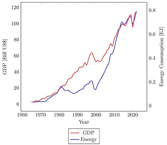
Figure 1. GDP and Energy Consumption for Ecuador.

There are outliers inside the data. Particularly, these data exist because there were sudden changes over time. For example, the 1999 bank crisis caused a deep decrease in the GDP and Energy Consumption. Something similar happened due to the COVID-19 pandemic. These data were treated with the inclusion of dummy variables, which is a technique used in econometrics to avoid influencing the structure of the data by paying exclusive attention to an outlier. Note that the outlier is not eliminated but is treated apart from the rest of the data.

Generally, the logarithm of the data was used. There is no obstacle in doing this because all the data are positive. This transformation has the advantage of reducing the range of the dependent variables and softening the exponential components of the time series.

3.2. Econometrics Model

In the end, the Granger test is the evaluation of a VAR model where both the GDP and Energy Consumption series are included and related. However, to have a dependable VAR model, both series must be well individually modelled.

The first thing that we must be sure of is that the series is stationary. The Unit Root test checks for this characteristic. In case the presence of a Unit Root is detected, we must determine if the trend is stochastic or deterministic. If it is the first case, the series is differentiated, and if it is the second case, the trend must be included in the model.

Then, in the correlogram of the stationary series (original or differentiated), we determine the possible model, AR or MA, and the lags that might be included. This is only a reference as the analysis of the model could change this.

The model is developed, e.g., ARIMA(1,1,1), and after that, the residuals are evaluated according to three concepts: an autocorrelation analysis, the autocorrelation of the squares, and normality. With these three characteristics, we are sure that the residuals are white noise and that no more information is kept inside them. After that, the impulse response is checked to see if the model is stable.

When the models for each time series (GDP and Economic Consumption) are well established, we include the variables into each other. This is the VAR model. We also analyse the residuals to see if they are not correlated if there is no heteroskedasticity and if they have a normal distribution. If the residuals are well behaved (spherical residuals) and if there is no Unit Root, the VAR model is accepted.

3.3. Causality Test

To determine if GDP growth causes Energy Consumption or vice versa, first of all, we compare the $AIC$ and the $SC$ values of the ARIMA and the VAR model. The better model has the lowest value. In other words, if the VAR model for GDP has a lower value of $AIC$ than that of the ARIMA GDP model, we can conclude that Energy Consumption causes GDP growth.

There is also the Granger test that is directly performed. In that case, the null hypothesis tests if the coefficients of the included variable are zero. If not, there exists Granger causality.

4. Results

4.1. Modelling the GDP

A simpler time-series model resulted when using the logarithm of the GDP instead of the original data, which is shown in Figure 2.

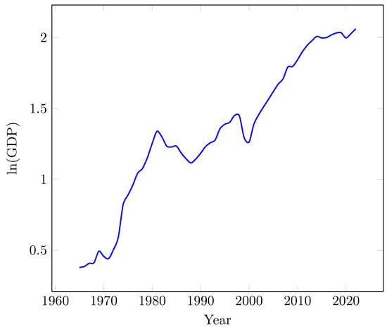
Figure 2. Logarithm of the GDP of Ecuador.

The Unit Root test for this series, considering only an intercept, shows a probability of 59.35% for $H0$. This means that the series is non-stationary. If a trend is added, the probability for $H0$ is 32.49%. The series is non-stationary with a stochastic trend.

The Unit Root test for the first difference, only with an intercept, shows that the probability for the null hypothesis $H0$ is 1.56%. Under a 5% level of confidence, the series could be considered stationary in its first difference, i.e., it is an $I\left(1\right)$ series.

The correlograms for the autocorrelation and the partial autocorrelation of the $I\left(1\right)$ series are shown in Figure 3a and Figure 3b, respectively. Note that in both correlograms, lag 1 is the most relevant. That characteristic suggests that the model might be an ARIMA(1,1,1). However, after some trial and error, the most suitable model was ARIMA(1,1,0).

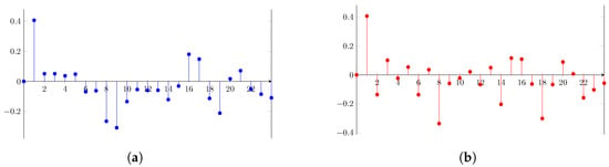
Figure 3. (a) Autocorrelation of the $I\left(1\right)$ series—GDP. (b) Partial autocorrelation of the $I\left(1\right)$ series—GDP.

The ARIMA(1,1,0) model cannot explain the behaviour of the GDP on its own. It fails in the normality of the residuals. Two outliers exist in the residual (Figure 4) and correspond to the years 1974 and 1999. The first outlier indicates the year when Ecuador began to export oil [27]. The second outlier shows the 1990s bank crisis.

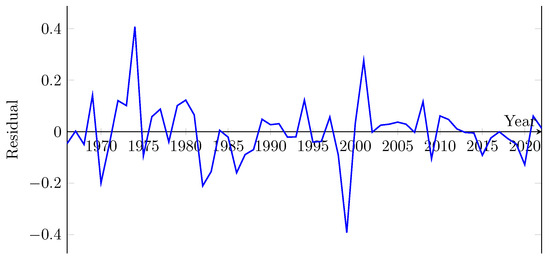
Figure 4. Residuals of the regression when no dummy variables are included.

To normalise the residuals, a dummy variable is included, specifically to aim at the outliers. The results are shown in Table 1. The coefficients of the variable AR(1) and the intercept C are significant. Only the dummy(-1) is not significant; however, this variable is kept so that the behaviour of the residuals is maintained.

Table 1. Regression results for the ARIMA(1,1,0) model of the GDP.

Variable	Coefficient	Std. Error	t-Statistic	Prob.
C	0.0744	0.0208	3.5710	0.0008
Dummy	−0.3175	0.0380	−8.3393	0
dummy(-1)	−0.0834	0.0806	−1.0348	0.3055
AR(1)	0.3926	0.1343	2.9234	0.0051
SIGMASQ	0.0076	0.0016	4.5908	0
R-squared	0.5114	Mean dependent var		0.0679
Adj. R-squared	0.4739	S.D. dependent var		0.1263
S.E. of regression	0.0916	Akaike info criterion		−1.855
Sum squared resid	0.4366	Schwarz criter.		−1.6762
Log likelihood	57.8808	Hannan–Quinn criter.		−1.7858
F-statistic	13.6110	Durbin–Watson stat.		1.9054
Prob (F-statistic)	0	Inverted AR Roots		0.39

The p-values for the autocorrelation of the residuals are shown in Figure 5. All of them are greater than 0.05, i.e., under 95% confidence, and the null hypothesis (H0: there is no correlation) is accepted. For the heteroskedasticity, the p-values for the squared residuals are also greater than 0.05 for all the cases, so the model does not present heteroskedasticity.

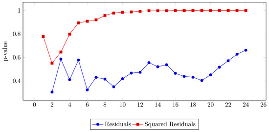
Figure 5. p-values for the residuals of the ARIMA(1,1,0) model for the GDP.

Now, we check the normality of the residuals. Once the dummy variables are introduced in the model, the distribution of the residuals is Gaussian, as the Jarque–Bera test shows under a probability of 79.65% (Figure 6a). The impulse response is shown in Figure 6b. The response is stabilised towards zero after a few periods, which is a sign that the phenomenon was modelled appropriately.

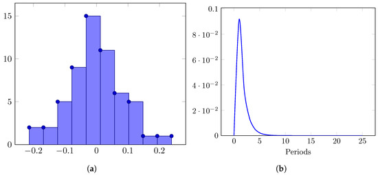
Figure 6. (a) Histogram of the residuals of the ARIMA(1,1,0) model for Ecuador. (b) Impulse response of the residuals of the ARIMA(1,1,0) model for Ecuador.

4.2. Modelling Energy Consumption

For Energy Consumption, the logarithmic transformation of the series was used. The Unit Root test, with interception only, gave a probability of 0.94% of H0. The time series is stationary.

The correlograms for the autocorrelation and partial autocorrelation of the time series are shown in Figure 7a,b. It is seen that the first term of the partial autocorrelation is the most relevant. We can assume a model ARIMA(1,0,0).

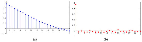
Figure 7. (a) Autocorrelation of the $I\left(1\right)$ series—Energy Consumption. (b) Partial autocorrelation of the $I\left(1\right)$ series—Energy Consumption.

In the regression results for ARIMA(1,0,0), a Unit Root was shown. This usually means that a difference is needed, although that was not evident in the initial Unit Root test. The regression results for the ARIMA(1,1,0) model are presented in Table 2. As happened with the GDP, for Energy Consumption, the dummy variables were needed too to normalise the residuals. The logarithmic model of Energy Consumption was stationary without any differentiation. As a consequence, the final model is almost a constant with noise, i.e., it is similar to white noise with media different from zero. This result is confirmed by the low R-squared and the low significance level of the AR(1) coefficient.

Table 2. Regression results for the ARIMA(1,0,1) model of Energy Consumption.

Variable	Coefficient	Std. Error	t-Statistic	Prob.
C	0.0591	0.0095	6.2418	0.0000
dummy	−0.1495	0.0455	−3.2872	0.0018
dummy(-1)	0.0082	0.0253	0.3229	0.7481
AR(1)	0.0205	0.1768	0.1161	0.9080
SIGMASQ	0.0035	0.0007	5.2052	0.0000
R-squared	0.2554	Mean dependent var		0.056656
Adj. R-squared	0.1981	S.D. dependent var		0.068727
S.E. of regression	0.0615	Akaike info criterion		−2.654476
Sum squared resid	0.1970	Schwarz criter.		−2.475261
Log likelihood	80.6526	Hannan–Quinn criter.		−2.584827
F-statistic	4.4582	Durbin–Watson stat.		1.994629
Prob (F-statistic)	0.0036	Inverted AR Roots		0.02

The p-values of the autocorrelation for the residuals and the squared residuals are shown in Figure 8. All of them show a probability greater than 5% for the null hypothesis, i.e., that there is no autocorrelation between the lags.

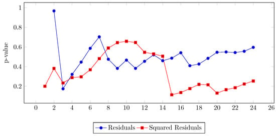
Figure 8. p-values for the residuals of the ARIMA(1,1,0) model for Energy Consumption.

The histogram of the residuals is shown in Figure 9a. The Jarque–Bera test gives a value of 4.28, i.e., a probability of 11.74% of H0: normal distribution, which, therefore, is accepted. The impulse test is shown in Figure 9b. The model is stable since it is damped in a few periods.

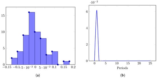
Figure 9. (a) Histogram of the residuals of the ARIMA(1,1,0) model for Energy Consumption. (b) Impulse response for the ARIMA(1,0,1) model of Energy Consumption.

4.3. VAR Model and Granger Causality Analysis

An analysis with two lags is performed. The results are shown in Table 3. If we compare the Akaike and the Schwarz criteria with those of the ARIMA models, we can verify that, when the energy is inserted in the GDP equation, the model improves. The case of EC is special since it improves with the inclusion of GDP; however, in the regression results, the coefficients were non-significant, so the analysis was not valid.

Table 3. Akaike and Schwarz criteria with and without the inclusion of the independent variable.

	GDP	GDP (EC)	EC	EC (GDP)
Akaike info criterion	−1.855	−1.8313	−2.6544	−2.5837
Schwarz criterion	−1.6762	−1.6123	−2.4752	−2.3647

Finally, the Granger test corroborates the fact that only Energy Consumption affects the GDP and not the other way around, see Table 4. H0 in this case means that the independent variable does not Granger cause the dependent variable. For the GDP, the probability of H0 is 1.75%; hence, H0 is rejected, and we can say that Energy Consumption Granger causes GDP. On the other hand, for Energy Consumption, the probability of H0 is 97.45%, so we accept the null hypothesis and consider that the GDP does not cause Energy Consumption.

Table 4. Granger test for the VAR model of Energy Consumption and GDP.

Dependent Variable: D (log(GDP))				Dependent Variable: D (log(energy))
Excluded	Chi-sq	df	Prob.	Excluded	Chi-sq	df	Prob.
D (log(energy))	8.0869	2	0.0175	D (log(GDP))	0.0516	2	0.9745

5. Conclusions

It was demonstrated that Energy Consumption Granger causes GDP growth and not the other way around. This result was confirmed by the Akaike Information Criterion and the Schwarz criterion, as well as the Grainger test itself. This result might help energy–economics planners in future activities towards the development of the economy of Ecuador.

In this research, data from Ecuador were exclusively used. This is a limitation since only 56 years were included. In a future study, panel data, which include relations with other countries of the region, might be employed. This could be an improvement due to the higher number of available data.

Through this research, the dependency of GDP growth on Energy Consumption was confirmed. This is an important result because it shows that policymakers must invest in energy infrastructure if they want to encourage an improvement in the Ecuadorian economy. The development of the electrical sector and better conditions for oil production may be seen as future implications of the results of this research.

One drawback of this study is that it is limited to the relationship between Energy Consumption and GDP. A more complete study should add other aspects of the macroeconomy, such as fiscal policy, productivity levels, technology development, etc.

References

- Beaudreau, B.C. On the methodology of energy-GDP Granger causality tests. Energy 2010, 35, 3535–3539. [Google Scholar] [CrossRef]
- Tiwari, A.K. The asymmetric Granger-causality analysis between energy consumption and income in the United States. Renew. Sustain. Energy Rev. 2014, 36, 362–369. [Google Scholar] [CrossRef]
- Mutascu, M. A bootstrap panel Granger causality analysis of energy consumption and economic growth in the G7 countries. Renew. Sustain. Energy Rev. 2016, 63, 166–171. [Google Scholar] [CrossRef]
- Chiou-Wei, S.Z.; Chen, C.F.; Zhu, Z. Economic growth and energy consumption revisited—Evidence from linear and nonlinear Granger causality. Energy Econ. 2008, 30, 3063–3076. [Google Scholar] [CrossRef]
- Sunde, T. Energy consumption and economic growth modelling in SADC countries: An application of the VAR Granger causality analysis. Int. J. Energy Technol. Policy 2020, 16, 41–56. [Google Scholar] [CrossRef]
- Tran, B.L.; Chen, C.C.; Tseng, W.C. Causality between energy consumption and economic growth in the presence of GDP threshold effect: Evidence from OECD countries. Energy 2022, 251, 123902. [Google Scholar] [CrossRef]
- Odhiambo, N.M. Trade openness and energy consumption in sub-Saharan African countries: A multivariate panel Granger causality test. Energy Rep. 2021, 7, 7082–7089. [Google Scholar] [CrossRef]
- Rahman, M.H.; Ruma, A.; Hossain, M.N.; Nahrin, R.; Majumder, S.C. Examine the empirical relationship between energy consumption and industrialization in Bangladesh: Granger causality analysis. Int. J. Energy Econ. Policy 2021, 11, 121–129. [Google Scholar] [CrossRef]
- Krkošková, R. Causality between energy consumption and economic growth in the V4 countries. Technol. Econ. Dev. Econ. 2021, 27, 900–920. [Google Scholar] [CrossRef]
- Bayar, Y.; Sasmaz, M.U.; Ozkaya, M.H. Impact of trade and financial globalization on renewable energy in EU transition economies: A bootstrap panel granger causality test. Energies 2020, 14, 19. [Google Scholar] [CrossRef]
- AlKhars, M.; Miah, F.; Qudrat-Ullah, H.; Kayal, A. A systematic review of the relationship between energy consumption and economic growth in GCC countries. Sustainability 2020, 12, 3845. [Google Scholar] [CrossRef]
- Sanchez-Loor, D.A.; Zambrano-Monserrate, M.A. Causality analysis between electricity consumption, real GDP, foreign direct investment, human development and remittances in Colombia, Ecuador and Mexico. Int. J. Energy Econ. Policy 2015, 5, 746–753. [Google Scholar]
- Cetin, M.; Ecevit, E. The dynamic causal links between energy consumption, trade openness and economic growth: Time series evidence from upper middle income countries. Eur. J. Econ. Stud. 2018, 7, 58–68. [Google Scholar]
- Yoo, S.H.; Kwak, S.Y. Electricity consumption and economic growth in seven South American countries. Energy Policy 2010, 38, 181–188. [Google Scholar] [CrossRef]
- Rodríguez-Caballero, C.V.; Ventosa-Santaulària, D. Energy-growth long-term relationship under structural breaks. Evidence from Canada, 17 Latin American economies and the USA. Energy Econ. 2017, 61, 121–134. [Google Scholar] [CrossRef]
- Apergis, N.; Payne, J.E. Energy consumption and growth in South America: Evidence from a panel error correction model. Energy Econ. 2010, 32, 1421–1426. [Google Scholar] [CrossRef]
- Jin, S.J.; Lim, S.Y.; Yoo, S.H. Causal relationship between oil consumption and economic growth in Ecuador. Energy Sources Part B Econ. Plan. Policy 2016, 11, 782–787. [Google Scholar] [CrossRef]
- Pinzón, K. Dynamics between energy consumption and economic growth in Ecuador: A granger causality analysis. Econ. Anal. Policy 2018, 57, 88–101. [Google Scholar] [CrossRef]
- Granger, C.W. Investigating causal relations by econometric models and cross-spectral methods. Econom. J. Econom. Soc. 1969, 37, 424–438. [Google Scholar] [CrossRef]
- Shojaie, A.; Fox, E.B. Granger causality: A review and recent advances. Annu. Rev. Stat. Its Appl. 2022, 9, 289–319. [Google Scholar] [CrossRef]
- Akaike, H. Akaike’s Information Criterion. In International Encyclopedia of Statistical Science; Lovric, M., Ed.; Springer: Berlin/Heidelberg, Germany, 2011; p. 25. [Google Scholar]
- Schwarz, G. Estimating the dimension of a model. Ann. Stat. 1978, 6, 461–464. [Google Scholar] [CrossRef]
- Gujarati, D.N.; Porter, D.C. Basic Econometrics, 5th ed.; McGraw-Hill: New York, NY, USA, 2009. [Google Scholar]
- Franses, P.H.; Dijk, D.V.; Opschoor, A. Time Series Models for Business and Economic Forecasting, 2nd ed.; Cambridge University Press: Cambridge, UK, 2014. [Google Scholar]
- Bank, W. World Bank National Accounts Data, and OECD National Accounts Data Files. 2024. Available online: https://data.worldbank.org (accessed on 2 May 2024).
- BP. Energy Outlook. 2024. Available online: https://www.bp.com (accessed on 5 May 2024).
- Quevedo, C. Ecuador: Petróleo y crisis económlca. In El Sector Energético Ecuatoriano y la Caída de los Precios Internacionales del Petróleo; FLACSO: Ciudad de Guatemala, Guatemala, 1986; pp. 91–150. [Google Scholar]
Disclaimer/Publisher’s Note: The statements, opinions and data contained in all publications are solely those of the individual author(s) and contributor(s) and not of MDPI and/or the editor(s). MDPI and/or the editor(s) disclaim responsibility for any injury to people or property resulting from any ideas, methods, instructions or products referred to in the content. |
© 2024 by the author. Licensee MDPI, Basel, Switzerland. This article is an open access article distributed under the terms and conditions of the Creative Commons Attribution (CC BY) license (https://creativecommons.org/licenses/by/4.0/).