Performance Assessment of Multi-RIS-Aided Localization in Non-Terrestrial Networks ^†

Abstract

The increasing demand for global connectivity has accelerated the integration of non-terrestrial networks (NTNs), particularly low Earth orbit (LEO) satellite constellations, into next-generation position navigation and time (PNT) systems. While LEO-based PNT offers low-latency and high-accuracy potential, challenges such as high path loss and limited ground-level signal diversity remain. Reconfigurable intelligent surfaces (RISs) have emerged as a cost-effective solution to enhance localization performance by providing controllable reflections with minimal infrastructure. Building on prior work in single-RIS NTN scenarios, this paper investigates RIS-aided localization in a single-LEO PNT setting with multiple RISs. We introduce a detailed signal model and multi-stage processing framework that estimates both the satellite and RIS-assisted paths, enabling accurate receiver localization. Simulations assess the trade-offs in coverage and accuracy, providing insights into the feasibility and optimization of RIS-assisted NTN PNT solutions as a complementary alternative to global navigation satellite system (GNSS).

1. Introduction

In recent years, the growing demand for ubiquitous connectivity has highlighted the limitations of traditional terrestrial network (TN), particularly in remote, rural, and underserved regions. NTNs have emerged as promising complementary solutions to enhance coverage and resilience in next-generation communication infrastructures [1]. In particular, the use of LEO satellite constellations has the potential to provide global 5G/6G coverage [2], and it has already shown the benefits of complementing existing GNSSs [3]. Now, the trend moves toward LEO-PNT solutions, benefiting from the high satellite dynamic, high-power signals, and low latencies [4,5]. Existing studies of LEO-PNT can be divided into multi-LEO PNT [4] or single-LEO PNT [6,7]. The former employs different types of signals, whereas the latter are focused on 5G orthogonal frequency division multiplexing (OFDM) signals.

We focus on single-LEO PNT relying on RISs as proposed in [7]. The use of RIS is a revolutionary way to provide additional, cost-effective location references/anchors. Unlike deploying base stations or satellites, RIS installations require minimal infrastructure while significantly improving localization accuracy and coverage. Current research primarily focuses on RIS-aided localization in TN systems, showing PNT capabilities with a single node [8]. Single node NTN localization is solved in [7] using a single RIS, but with small coverage area in the vicinity of the RIS. The high attenuation of the satellite–RIS–receiver path limits performance over long distances of the receiver from the RIS. This challenge can be addressed by deploying multiple RIS, as indicated by several sources on TN [9,10,11]. Research on multiple RISs for an NTN is limited to performance bounds and using multiple satellites [12,13].

In this paper, inspired by [7,10], we address the problem of single-LEO PNT with the aid of multiple RISs. We consider an OFDM signal to serve as alternative PNT solution for GNSS. The contributions of this work are twofold: (i) introducing a signal model and processing techniques for NTN RIS-aided localization with multiple RIS; and (ii) describing and analyzing a multi-stage estimator able to obtain the satellite and RISs channel paths and corresponding receiver position. Specifically, Section 2 introduces the system model, Section 3 describes the positioning algorithm using multiple RISs. Finally, Section 4 shows the numerical results, and Section 5 concludes this paper.

2. System Model

We consider a three-dimensional (3D) user localization problem in a single-antenna NTN system consisting of one LEO satellite and $R>1$ RISs in the vicinity of the user’s receiver, as depicted in Figure 1. In this system, a moving user in an unknown position receives downlink signals from both the satellite direct channel and the satellite–RISs reflection channels, and then performs position estimation. Furthermore, the receiver needs synchronization because the clocks of the satellite and the receiver are assumed to have an unknown time offset $\delta t$. This section initially introduces the underlying geometric relationship present in the system under consideration, followed by the signal model used. Subsequently, we detail the system setup.

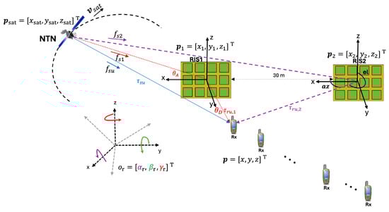
Figure 1. Illustration of the considered LEO-PNT system with R RISs.

2.1. Geometry Model and Channel Parameters

We assume the receiver is in movement with unknown velocity $\mathbf{v}\in {\mathbb{R}}^3$ and has an unknown location $\mathbf{p}\in {\mathbb{R}}^3$, whereas during the measurement time the satellite has known location ${\mathbf{p}}_{\mathrm{sat}}\left(t\right)$ and velocity ${\mathbf{v}}_{\mathrm{sat}}\left(t\right)$. The RISs have known locations (array centers) ${\mathbf{p}}_r\in {\mathbb{R}}^3$, and a known orientation described by Euler angle vectors ${\mathbf{o}}_r\in {\mathbb{R}}^3$ for $r=1,2,\dots ,R$. All the RISs consist of a uniform rectangular array (URA) with $N=N_x\times N_z$ elements, where $N_x$ and $N_z$ are the number of the RIS elements placed along its local x- and z-axes, respectively. The n-th element of the RIS is located at ${\mathbf{p}}_{\mathrm{El},n}\in {\mathbb{R}}^3$ in the local coordinate frame (LCF) of the RIS. The RIS elements are spaced by $\lambda /2$, where $\lambda \doteq c/f_{\mathrm{c}}$ is the wavelength, $f_{\mathrm{c}}$ is the carrier frequency, and c is the speed of light. We define rotation matrices ${\mathbf{R}}_r=\mathbf{R}\left({\mathbf{o}}_r\right)\in SO\left(3\right)$ described by Euler angle vectors ${\mathbf{o}}_r={[{\alpha }_r,{\beta }_r,{\gamma }_r]}^{\top }$ [14]. Specifically, a given vector $\mathbf{x}$ at the global coordinate frame (GCF) can be expressed at the RIS body frame as ${\mathbf{R}}_r^{\top }\mathbf{x}$. Similar for the satellite but using ${\mathbf{R}}_{\mathrm{sat}}\doteq \mathbf{R}\left({\mathbf{o}}_{\mathrm{sat}}\right)$. Such rotations can be determined as in [13,14,15].

The position and velocity of LEO satellites can be described by the orbit dynamic defined by Keplerian parameters $\mathsf{\Omega }=\{h,\psi ,{\mathbf{o}}_{\mathrm{sat}}\}$ [16]. The orbit height h and the Keplerian angles ${\mathbf{o}}_{\mathrm{sat}}$ define the position of the orbit plane in the GCF, while the elevation angle $\psi$ specifies the position in the orbit LCF. Once this position is determined by ${\tilde{\mathbf{p}}}_{\mathrm{sat}}\left(t\right)$, we can express it at the GCF by [16]: ${\mathbf{p}}_{\mathrm{sat}}\left(t\right)={\mathbf{R}}_{\mathrm{sat}}{\tilde{\mathbf{p}}}_{\mathrm{sat}}\left(t\right)-{[0,0,R_{\mathrm{E}}]}^{\top }$ with $R_{\mathrm{E}}$ the Earth radius. Now, let ${\mathcal{C}}_{\vartheta }$ and ${\mathcal{S}}_{\vartheta }$ with $\vartheta \in \{\alpha ,\beta ,\gamma \}$ be shorthand notations for $cos\left(\vartheta \right)$ and $sin\left(\vartheta \right)$, respectively. Then, the satellite position at the orbit LCF for elevation angle ${\psi }_{t_0}$ is given by ${\tilde{\mathbf{p}}}_{\mathrm{sat}}\left(t\right)=R_{\mathrm{c}}{\left[{\mathcal{C}}_{{\psi }_t},{\mathcal{S}}_{{\psi }_t},0\right]}^{\top }$, where $R_{\mathrm{c}}=R_{\mathrm{E}}+h$ is the constellation radius. Then, it can be updated every time interval $T>0$ as ${\tilde{\mathbf{p}}}_{\mathrm{sat}}(t_0+T)={\tilde{\mathbf{p}}}_{\mathrm{sat}}\left(t_0\right)+{\tilde{\mathbf{v}}}_{\mathrm{sat}}\left(t_0\right)T$, where ${\tilde{\mathbf{v}}}_{\mathrm{sat}}\left(t\right)={\omega }_{\mathrm{sat}}{R}_{\mathrm{c}}{\left[-{\mathcal{S}}_{{\psi }_t},{\mathcal{C}}_{{\psi }_t},0\right]}^{\top }$, ${\omega }_{\mathrm{sat}}=\sqrt{F_m/R_{\mathrm{c}}^3}$ with $F_m=4.0038·{10}^{14}$ m³/s², and ${\psi }_t\doteq arctan({\left[{\tilde{\mathbf{p}}}_{\mathrm{sat}}\left(t\right)\right]}_2/{\left[{\tilde{\mathbf{p}}}_{\mathrm{sat}}\left(t\right)\right]}_1)$.

For the direct channel path, we are mainly interested in two parameters: the Doppler shift, and the time delay. These parameters are given by $f_0=\left[{({\mathbf{v}}_{\mathrm{sat}}-\mathbf{v})}^{\top }(\mathbf{p}-{\mathbf{p}}_{\mathrm{sat}})\right]/\left(\lambda \left|\left|\mathbf{p}-{\mathbf{p}}_{\mathrm{sat}}\right|\right|\right)$, and ${\tau }_0=\left|\left|\mathbf{p}-{\mathbf{p}}_{\mathrm{sat}}\right|\right|/c+\delta t$, respectively, where $\delta t$ is an unknown but fixed clock bias between the LEO satellite and the receiver. For the reflected paths, we have to consider R different channel paths with Doppler and time delay given by

$$\begin{array}{cc}\hfill f_{\mathrm{r}}& \doteq f_{\mathrm{sr}}+f_{\mathrm{ru}}={\displaystyle \frac{{\mathbf{v}}_{\mathrm{sat}}^{\top }\left({\mathbf{p}}_{\mathrm{sat}}-{\mathbf{p}}_r\right)}{\lambda \left|\left|{\mathbf{p}}_{\mathrm{sat}}-{\mathbf{p}}_r\right|\right|}}+{\displaystyle \frac{{\mathbf{v}}^{\top }\left({\mathbf{p}}_r-\mathbf{p}\right)}{\lambda \left|\left|{\mathbf{p}}_r-\mathbf{p}\right|\right|}},\hfill \\ \hfill {\tau }_r& \doteq {\tau }_{\mathrm{sr}}+{\tau }_{\mathrm{ru}}={\displaystyle \frac{\left|\left|{\mathbf{p}}_{\mathrm{sat}}-{\mathbf{p}}_r\right|\right|+\left|\left|{\mathbf{p}}_r-\mathbf{p}\right|\right|}{c}}+\delta t,\hfill \end{array}$$

(1)

with $\{f_{\mathrm{sr}},{\tau }_{\mathrm{sr}}\}$ the Doppler and time delay between satellite and RIS, and $\{f_{\mathrm{ru}},{\tau }_{\mathrm{ru}}\}$ between RIS and receiver. In this case, we additionally have to consider angle of arrival (AoA) and angle of departure (AoD) at and from the different RISs, respectively. Note that in 3D space, each of these angles consists of an azimuth, $\varphi$, and elevation angle, $\theta$, as defined in Figure 1. Let ${\mathsf{\phi }}_{g,r}\doteq {[{\varphi }_{g,r},{\theta }_{g,r}]}^{\top }$ with $g=\{\mathrm{A},\mathrm{D}\}$ be the AoA and AoD at the r-th RIS. Then, these angles can be expressed as

$${\mathsf{\phi }}_{g,r}={\left[arctan\left({\left[{\mathbf{R}}_r^{\top }\Delta {\mathbf{p}}_{gr}\right]}_2/{\left[{\mathbf{R}}_r^{\top }\Delta {\mathbf{p}}_{gr}\right]}_1\right),arcsin\left({\left[{\mathbf{R}}_r^{\top }\Delta {\mathbf{p}}_{gr}\right]}_3/\left|\left|\Delta {\mathbf{p}}_{gr}\right|\right|\right)\right]}^{\top },$$

(2)

where $\Delta {\mathbf{p}}_{gr}={\mathbf{p}}_r-{\mathbf{p}}_g$, with ${\mathbf{p}}_g=\{{\mathbf{p}}_{\mathrm{sat}},\mathbf{p}\}$, denotes the vector from the r-th RIS to satellite (for $g=\mathrm{A}$) or to receiver (for $g=\mathrm{D}$), respectively, in the GCF. Note all angles are computed in the LCF of each RIS, thus we use the corresponding rotation matrix ${\mathbf{R}}_r$.

2.2. Signal Model

We consider OFDM signals transmitted from the satellites with K subcarriers and total symbol duration $T_{\mathrm{sym}}=T+T_{\mathrm{CP}}$, where $T=1/{\Delta }_f$ is the elementary symbol duration, ${\Delta }_f=B/K$ is the subcarrier spacing with B the signal bandwidth, and $T_{\mathrm{CP}}$ is the cyclic prefix (CP) duration. In this subsection we will consider the transmission and reception of one symbol only. The complex baseband signal for the l-th transmitted symbol is written as

$$s\left(t\right)=\sqrt{{\displaystyle \frac{P_{\mathrm{s}}}{K}}}\sum _{k=0}^{K-1}{x}_{k,l}{e}^{j2\pi k{\Delta }_f\left(t-l{T}_{\mathrm{sym}}\right)}g\left(t-l{T}_{\mathrm{sym}}\right),$$

(3)

where $P_{\mathrm{s}}$ denotes the total signal power, $x_{k,l}\in \mathbb{C}$ is the l-th transmitted pilot symbol on the k-th subcarrier, $g\left(t\right)=1$ when $t\in [0,T_{\mathrm{sym}}]$, and 0 otherwise. The transmitted passband signal is $s_{\mathrm{PB}}\left(t\right)=\Re \{s\left(t\right)exp\left(j2\pi f_{\mathrm{c}}t\right)\}$. To describe the received signal model we consider the direct line-of-sight (LoS) path between satellite and receiver, and the reflected paths between satellite–RISs–receiver. The received baseband signal after downconversion wassampled at $t=l{T}_{\mathrm{sym}}+T_{\mathrm{CP}}+\kappa T/K$, with $\kappa =0,1,\dots ,K-1$; the discrete-time signal for the l-th symbol was $r\left[\kappa \right]=r_{\mathrm{LoS}}\left[\kappa \right]+r_{\mathrm{RIS}}\left[\kappa \right]+n\left[\kappa \right]$, with $n\left[\kappa \right]$ a thermal noise with power spectral density $N_0$.

Now, let ${\alpha }_i$, ${\tau }_i$, $f_i$, ${\mathsf{\Phi }}_r=[{\mathsf{\phi }}_r^{\left(\mathrm{A}\right)},{\mathsf{\phi }}_r^{\left(\mathrm{D}\right)}]$ with $i=\{0,r\}$ and $r=1,\dots ,R$ be the channel amplitude, time delay, Doppler frequency, and AoA/AoD of the i-th path (with $i=0$ for the LoS path), and ${\upsilon }_i=f_i/f_{\mathrm{c}}$. Then, the discrete-time signal for the l-th symbol is [7]

$$\begin{array}{cc}\hfill r_{\mathrm{LoS}}\left[\kappa \right]& =\sqrt{{\displaystyle \frac{P_{\mathrm{s}}}{K}}}{\alpha }_0{e}^{j2\pi f_0\left(\kappa T/K\right)}\sum _{k=0}^{K-1}{x}_{k,l}{e}^{j2\pi k\kappa /K}{e}^{j2\pi f_{0}l{T}_{\mathrm{sym}}}{e}^{-j2\pi k{\Delta }_f\left({\tau }_0-{\upsilon }_{0}l{T}_{\mathrm{sym}}\right)},\hfill \\ \hfill r_{\mathrm{RIS}}\left[\kappa \right]& =\sqrt{{\displaystyle \frac{P_{\mathrm{s}}}{K}}}\sum _{r=1}^R{\alpha }_r{G}_{r,l}\left({\mathsf{\Phi }}_r\right)e^{j2\pi f_{\mathrm{r}}\left(\kappa T/K\right)}\sum _{k=0}^{K-1}{x}_{k,l}{e}^{j2\pi k\kappa /K}{e}^{j2\pi f_{\mathrm{r}}l{T}_{\mathrm{sym}}}{e}^{-j2\pi k{\Delta }_f\left({\tau }_r-{\upsilon }_{r}l{T}_{\mathrm{sym}}\right)},\hfill \end{array}$$

(4)

where $G_{rl}\left({\mathsf{\Phi }}_r\right)\in \mathbb{C}$ is the r-th RIS beamforming gain, which accounts for the AoA and AoD is modeled by the steering vector $\mathbf{a}\left(\mathsf{\phi }\right)$, and the RIS phase profile is modeled by ${\mathit{\omega }}_r\left(t\right)={[{\omega }_{r,1},\dots ,{\omega }_{r,R}]}^{\top }$. Let ⊙ be the element-wise matrix multiplication; then this gain is

$$G_r(t;{\mathsf{\Phi }}_r)={\left[\mathbf{a}\left({\mathsf{\phi }}_r^{\left(\mathrm{A}\right)}\right)\odot \mathbf{a}\left({\mathsf{\phi }}_r^{\left(\mathrm{D}\right)}\right)\right]}^{\top }{\mathit{\omega }}_r\left(t\right)=\sum _{n=1}^N{e}^{-j2\pi f_{\mathrm{c}}{\tau }_n\left({\mathsf{\phi }}_r^{\left(\mathrm{A}\right)}\right)}{e}^{-j2\pi f_{\mathrm{c}}{\tau }_n\left({\mathsf{\phi }}_r^{\left(\mathrm{D}\right)}\right)}{e}^{{\omega }_{r,n}\left(t\right)}.$$

(5)

Note the RIS’s steering vector is modeled as ${\left[\mathbf{a}\left(\mathsf{\phi }\right)\right]}_n=exp(-j2\pi f_{\mathrm{c}}{\tau }_n\left(\mathsf{\phi }\right))$, and ${\tau }_n\left(\mathsf{\phi }\right)$ captures the time-shift produced by the reflection of the signal at the n-th RIS element (compared to the RIS center). This is given by ${\tau }_n\left(\mathsf{\phi }\right)=-\left({\mathbf{p}}_{\mathrm{El},n}^{\top }\mathbf{k}\left(\mathsf{\phi }\right)\right)/c$ with $\mathbf{k}\left(\mathsf{\phi }\right)={[{\mathcal{C}}_{\varphi }{\mathcal{C}}_{\theta },{\mathcal{S}}_{\varphi }{\mathcal{C}}_{\theta },{\mathcal{S}}_{\theta }]}^{\top }$, the direction vectors in the LCF of the r-th RIS corresponding to angle $\mathsf{\phi }$.

2.3. System Setup

In general, the channel parameters are all functions of time t, as they depend on the varying location of the satellite. However, we will operate under conditions for which the parameters remain constant within samples, but they vary between different symbols. We also assume that the RIS phase configurations change every symbol. For the estimation process, we consider the reception of L OFDM symbols, and we insert the time-variation in parameters into (4) by letting ${\mathbf{r}}_l\doteq {[r_l\left[0\right],\dots ,r_l[K-1]]}^{\top }$ be the K samples received at the l-th symbol, and the subindex l denoting the temporal dependence of channel parameters in (4). Furthermore, we use ${\mathbf{x}}_i={[x_{i,1},x_{i,2},\dots ,x_{i,L}]}^{\top }$ to denote the temporal variation in parameter $x_i$. So, collecting the K samples of the L received symbols in matrix form, the received signal can be rewritten with $\{{\mathbf{Y}}_{\mathrm{LoS}},{\mathbf{Y}}_{\mathrm{RIS}}\}\in {\mathbb{C}}^{K\times L}$.

To do so, let $\mathbf{F}\in {\mathbb{C}}^{K\times K}$ be the unitary fast Fourier transform (FFT) matrix with elements ${\left[\mathbf{F}\right]}_{k,m}=(1/\sqrt{K})exp(-j2\pi km/K)$, $\mathbf{X}\in {\mathbb{C}}^{K\times L}$ the transmitted pilot symbols, and ${\mathbf{A}}_i$ includes the signal power and propagation attenuation factor. Then,

$$\begin{array}{cc}\hfill {\mathbf{Y}}_{\mathrm{LoS}}& ={\mathbf{A}}_0\mathbf{E}\left({\mathbf{f}}_0\right)\odot {\mathbf{F}}^H\left(\mathbf{C}\left({\mathbf{f}}_0\right)\odot \mathbf{D}\left({\tau }_0\right)\odot \mathbf{X}\right),\hfill \\ \hfill {\mathbf{Y}}_{\mathrm{RIS}}& =\sum _{r=1}^R{\mathbf{A}}_r\mathbf{E}\left({\mathbf{f}}_{\mathrm{r}}\right)\odot {\mathbf{F}}^H\left(\mathbf{C}\left({\mathbf{f}}_{\mathrm{r}}\right)\odot \mathbf{D}\left({\tau }_r\right)\odot {\mathbf{G}}_r\left({\tilde{\mathsf{\Phi }}}_r\right)\odot \mathbf{X}\right),\hfill \end{array}$$

(6)

with ${\left[\mathbf{E}\left({\mathbf{f}}_i\right)\right]}_{\kappa ,l}=exp(j2\pi f_i\kappa /\left(KT\right))$,${\left[\mathbf{D}\left({\tau }_i\right)\right]}_{\kappa ,l}=exp(-j2\pi {\Delta }_f\kappa ({\tau }_i-{\upsilon }_{i}l{T}_{\mathrm{sym}}))$, ${\left[\mathbf{C}\left({\mathbf{f}}_i\right)\right]}_{\kappa ,l}=exp\left(j2\pi f_{i}l{T}_{\mathrm{sym}}\right)$, and ${\left[{\mathbf{G}}_r\left({\tilde{\mathsf{\Phi }}}_r\right)\right]}_{\kappa ,l}=G_{r,l}\left({\mathsf{\Phi }}_{r,l}\right)$ with ${\tilde{\mathsf{\Phi }}}_r=[{\mathsf{\Phi }}_{r,1},\dots ,{\mathsf{\Phi }}_{r,L}]$ for $\kappa =0,\dots ,K-1$, $l=0,\dots ,L-1$, and $i=\{0,r\}$ with $r=1,\dots ,R$. Combining the received components in (6), the received signal samples can be written in compact form as $\mathbf{Y}={\mathbf{Y}}_{\mathrm{LoS}}+{\mathbf{Y}}_{\mathrm{RIS}}+\mathbf{N}$ with $\mathbf{N}\in {\mathbb{C}}^{K\times L}$ capturing the noise effects.

3. Multi-RIS-Aided LEO-PNT Algorithm

Our goal is to estimate the receiver position, $\mathbf{p}$, from the received signal $\mathbf{Y}$. To do this, we first estimate the LoS channel parameters and those of the path arriving from the different RISs. For this, we use the design freedom of the RIS in terms of phase profile, ${\mathit{\omega }}_r\left(t\right)$, to avoid interference from different paths. Second, we use the estimated parameters to extract the receiver position based on time delay and AoD measures. In this section, we first describe the design of RIS phase profile that allows us to decouple the received signals from different paths (i.e., LoS and RISs). Then, based on the received signals we explain the channel parameter estimation, and finally we also describe the position estimation process based on the channel parameter estimates.

3.1. RIS Phase Profile Design

We assume that the RIS phase profiles are always known at the receiver, and we design them to avoid interference between the different reflected paths [10]. To do so, we first divide the total transmission of L OFDM symbols into $\tilde{L}$ slots of $P\ge R+1$ consecutive (symbol time) intervals, i.e., $L=P·\tilde{L}$. Then, at each slot $g=0,1,\dots ,\tilde{L}-1$ we generate the slow-varying part of the phase profile, ${\mathit{\zeta }}_{r,g}\in {\mathbb{C}}^{N\times 1}$, and we repeat it P consecutive symbol times. Furthermore, we use the matrix $\mathbf{B}\in {\mathbb{C}}^{P\times (R+1)}$ to describe the fast-varying part of the phase profile within the P consecutive symbols at each slot. Now, let $l=gP+p$ with $p=1,\dots ,P$, $B_{r,p}={\left[\mathbf{B}\right]}_{r,p}$, so that we can write the r-th RIS phase profile for the l-th symbol, ${\mathit{\omega }}_{r,l}={\mathit{\omega }}_r\left(l{T}_{\mathrm{sym}}\right)$, as

$${\mathit{\omega }}_{r,gP+p}=B_{r,p}{\mathit{\zeta }}_{r,g}.$$

(7)

The fast-varying part of the phase profile is designed to be (time-) orthogonal between RISs and LoS, so the columns of matrix $\mathbf{B}=[{\mathbf{b}}_0,{\mathbf{b}}_1,\dots ,{\mathbf{b}}_R]$ are designed to be orthogonal. To do so, we get ${\mathbf{b}}_r$ as the r-th column of Butson-type Hadamard matrices [11]. Now, let ${\mathbf{Z}}_r\in {\mathbb{C}}^{K\times \tilde{L}}$ be the received signal from the r-th path for the $\tilde{L}$ slots. Then, the LoS path (for $r=0$) and all the RIS paths (for $1\le r\le R$) can be separated every slot g as

$${\left[{\mathbf{Z}}_r\right]}_{:,g}={\displaystyle \frac{1}{P}}\left({\left({\mathbf{X}}^{\left(g\right)}\right)}^{*}\odot {\mathbf{Y}}^{\left(g\right)}\right){\mathbf{b}}_r^{*},$$

(8)

with ${\mathbf{Y}}^{\left(g\right)}\in {\mathbb{C}}^{K\times P}$ the received signal during the P consecutive intervals for the g-th slot. For the slow-varying part, we have freedom to select ${\mathit{\zeta }}_{r,g}$ for each RIS and transmission slot $g=0,\dots ,\tilde{L}-1$. The choice of ${\mathit{\zeta }}_{r,g}$ could correspond [10], e.g., to $\tilde{L}$ different beams that are directed to the receiver (e.g., if some prior knowledge of the receiver position is available); or to cover a plurality of users; or random beams to provide omnidirectional illumination. It is important to recall that ${\mathit{\zeta }}_{r,g}$ only needs to be generated for $0\le g\le \tilde{L}-1$ for the different RISs. The rest of the $L-\tilde{L}$ phase profiles can be generated based on (7).

3.2. Channel Parameter Estimation

In this section, we propose an estimator to get first the channel parameters and then (in next section) the receiver position and clock bias based on them. The unknown channel parameters comprise a total of $3+4·R$ parameters, so that a ($3+4·R$)-D maximum likelihood estimator (MLE) would be needed to obtain an optimal solution. To reduce complexity, we treat ${\mathbf{Z}}_r$ as if it only constitutes the effects of the r-th path (with $r=0$ for LoS), and proceed with estimating the r-th path channel parameters. For the estimation of the direct path channel parameters we perform a 2D correlation of the received signal with a local replica of (4) matched with tentative values of the direct path channel parameters. Let ${\tilde{s}}_{\kappa ,l}(\tau ,f)$ be this local replica, and ${\left[\mathbf{d}\left(\tau \right)\right]}_{\kappa }=exp(-j2\pi k{\Delta }_f\tau )$. So, the correlation function is

$$R_{\tau ,f}=\sum _{l=0}^{L-1}\sum _{\kappa =0}^{K-1}{r}_g\left[\kappa \right]{\tilde{s}}_{\kappa ,l}^{*}(\tau ,f)={\mathbf{d}}^H\left(\tau \right){\mathbf{Y}}_f{\mathbf{c}}^{*}\left(f\right),$$

(9)

where ${\left[\mathbf{c}\right]}_l=exp\left(j2\pi fl{T}_{\mathrm{sym}}\right)$, and letting ${\left[{\mathbf{D}}_f^{*}\right]}_{\kappa ,l}=exp\left(j2\pi \kappa {\Delta }_{f}fl{T}_{\mathrm{sym}}\right)$

$${\mathbf{Y}}_f={\mathbf{D}}_f^{*}\odot \mathbf{F}\left({\mathbf{E}}^{*}\left(f\right)\odot \mathbf{Y}\right).$$

(10)

To estimate the LoS parameters we use ${\mathbf{Z}}_0\left(f\right)=match\left({\mathbf{Y}}_f\right)$ as given by (8) to remove interferences of other paths, and we perform the 2D search of the correlation function as

$$\left[{\widehat{\tau }}_0,{\widehat{f}}_0\right]=arg\underset{\tau ,f}{max}\left\{|R_{\tau ,f}|\right\}=arg\underset{\tau ,f}{max}\left\{|{\mathbf{d}}^H\left(\tau \right){\mathbf{Z}}_0\left(f\right){\mathbf{c}}^{*}\left(f\right)|\right\}.$$

(11)

It is worth highlighting that effects of $\tau$ only varies the rows of ${\mathbf{Z}}_0$, while Doppler only affects its columns, so parameters can be decoupled from the maximization of the correlation function. This allows us to estimate the delay and Doppler either directly via a 2D-FFT [7] or by two separate 1D-FFT with non-coherent integration [8]. The FFT will provide a coarse estimation, which can be refined with some numerical optimization algorithm using the coarse estimation as the initial state of the optimization (e.g., Newton–Raphson).

The first step toward estimating the RIS-path channel parameters is to eliminate the LoS path component from $\mathbf{Y}$, using the estimated LoS channel parameters. Furthermore, we remove the interference of other RIS paths so that we have their estimations available.

Then, we consider $f_{\mathrm{sr}}\approx f_0$ and set ${\widehat{f}}_{\mathrm{r}}={\widehat{f}}_0+{\widehat{f}}_{\mathrm{ru}}$. Let the signal after interference cancellation be ${\tilde{\mathbf{Y}}}_r$. Next, we compensate for the satellite Doppler effect by computing ${\tilde{\mathbf{Y}}}_{{\widehat{f}}_{\mathrm{sr}}}$ as in (10) with using ${\tilde{\mathbf{Y}}}_r$ instead of $\mathbf{Y}$. For the estimation of the r-th path we use ${\mathbf{Z}}_r=match\left({\tilde{\mathbf{Y}}}_{{\widehat{f}}_{\mathrm{sr}}}\right)$ to remove interferences of other paths. With this setting, and based on the result in (9), the correlation function of the r-th RIS path is written as

$$R_{\tau ,f}\left(\mathsf{\phi }\right)={\mathbf{d}}^H\left(\tau \right){\mathbf{Z}}_r{\left[\mathbf{c}\left(f\right)\odot {\mathbf{g}}_r\left(\mathsf{\phi }\right)\right]}^{*},$$

(12)

with ${\mathbf{g}}_r\left(\mathsf{\phi }\right)\in {\mathbb{C}}^{\tilde{L}\times 1}$ the RIS beamforming gain for the $\tilde{L}$ slots as given in (5).

The effect of $\{f,\mathsf{\phi }\}$ is the same for all rows of ${\mathbf{Z}}_r$, which allows us to separate the estimation in two independent optimizations. First, the time delay:

$$\widehat{{\tau }_r}=arg\underset{\tau }{max}\left\{\sum _{l=1}^{\tilde{L}}\left|{\mathbf{d}}^H\left(\tau \right){\left[{\mathbf{Z}}_r\right]}_{:,l}\right|\right\}.$$

(13)

Second, once the time delay is compensated with ${\mathbf{z}}_r={\mathbf{Z}}_r^{\top }{\mathbf{d}}^{*}\left(\widehat{{\tau }_r}\right)$, we get

$$\left[{\widehat{f}}_{\mathrm{ru}},{\widehat{\mathsf{\phi }}}_{\mathrm{D}}\right]=arg\underset{f,\mathsf{\phi }}{max}\left\{|{\mathbf{c}}^H\left(f\right)\left({\mathbf{z}}_r\odot {\mathbf{g}}_r^{*}\left(\mathsf{\phi }\right)\right)|\right\},$$

(14)

and finally ${\widehat{f}}_{\mathrm{r}}={\widehat{f}}_0+{\widehat{f}}_{\mathrm{ru}}$. The previous optimization can be performed by providing candidate values for $\mathsf{\phi }$ and performing the maximization using FFT. Furthermore, for the candidate values of $\mathsf{\phi }$ and the corresponding ${\mathbf{g}}_r\left(\mathsf{\phi }\right)$ a 2-FFT approach can be followed [8]. A refined version can be obtained numerically.

3.3. Position Estimation

The receiver’s position $\mathbf{p}$ is estimated jointly from the geometric parameters obtained at multiple RISs. For each ${\mathbf{p}}_r$, the direction from the RIS to the user is first determined from the estimated angles ${\widehat{\mathsf{\phi }}}_{\mathrm{D}}$, which define a unit vector ${\mathbf{K}}_r=\mathbf{k}\left({\widehat{\mathsf{\phi }}}_{\mathrm{D}}\right)$. The user position is then computed by minimizing the cost function

$$f(\mathbf{p},\Delta t)=\sum _{r=1}^{N_{\mathrm{RIS}}}{\left(\parallel \mathbf{p}-{\mathbf{p}}_r\parallel -c({\widehat{\tau }}_k-\Delta t)\right)}^2+{\left(1-{\mathbf{K}}_r^{\top }{\displaystyle \frac{\mathbf{p}-{\mathbf{p}}_r}{\parallel \mathbf{p}-{\mathbf{p}}_r\parallel }}\right)}^2,$$

(15)

which enforces consistency with both the estimated delays ${\widehat{\tau }}_k$ and angles ${\widehat{\mathsf{\phi }}}_{\mathrm{D}}$, while estimating the user position and clock bias. The solution $(\widehat{\mathbf{p}},\widehat{\Delta t})$ is obtained via nonlinear least squares, initialized at the centroid of the RIS positions.

4. Simulation Results

This section evaluates the position accuracy and coverage performance of the NTN scenario, considering both single- and multi-RIS configurations. The simulation setup comprises a satellite transmitter, two RISs and a single-antenna receiver as depicted in Figure 1. The scenario considers a satellite orbit with a pitch angle ${\theta }_{\mathrm{PG}}={90}^{\circ }$, inclination ${\theta }_{\mathrm{I}}={81}^{\circ }$ and ascending node angle ${\theta }_{\mathrm{AN}}=\pm {45}^{\circ }$. To demonstrate the potential of RIS in enhancing positioning accuracy and system coverage, the satellite motion is isolated by setting the satellite elevation at $\psi ={{10}^{-4}}^{\circ }$. At this position, the satellite has the maximum carrier-to-noise ratio (CN0) around 69 dB-Hz. The two RISs are deployed at fixed terrestrial locations: one at the origin and the other 30 m apart along the x-axis. Results are obtained using $f_{\mathrm{c}}=1.462$ GHz, and assuming that the user resides within the far-field of each RIS. Furthermore, ${\Delta }_f=60$ kHz with $K=1333$ subcarriers (i.e., a total of 80 MHz bandwidth). A random RIS phase profile is considered for all the following results. The rest of the simulation parameters can be found in Table 1.

Table 1. Default simulation parameters.

Types	Simulation Parameters
TX Position (m)	${\mathbf{p}}_{sat}={[-0.8383\times {10}^6,0.8383\times {10}^6,1.1067\times {10}^6]}^{\top }$
RIS Positions (m)	${\mathbf{p}}_1={[0,0,0]}^{\top },{\mathbf{p}}_2={[-30,0,0]}^{\top }$
RIS Orientation	${\mathbf{o}}_1={[0,0,0]}^{\top },{\mathbf{o}}_2={[0,0,0]}^{\top }$
RIS Size	$N=64\times 64$
Carrier Frequency	$f_c=1.462$ GHz
Bandwidth	$BW=80$ MHz
Number of Transmissions	$L=256$
Number of Subcarriers	$K=1333$
Average Transmission Power	$P=63$ dBm
Noise PSD	$N_0=-174$ dBm/Hz
Noise Figure	8 dB

4.1. Performance Analysis

The performance is analyzed along a user trajectory ${\left[-r/\sqrt{2},r/\sqrt{2},-10\right]}^{\top }$ with $r\in [2,100]$ m, averaging results over 100 random realizations of RIS phase profiles and noise. Both single- and multi-RIS scenarios are compared against the Cramér–Rao lower bound (CRLB) in Figure 2. For small r, RIS 1 dominates due to proximity and favorable angles, while RIS 2 has minimal impact. As r increases, RIS 1 weakens, and RIS 2 becomes more effective due to improved geometry. Delay estimation errors follow this trend, tracking the CRLB at low/intermediate r for RIS 1, but degrading for RIS 2, and vice versa at large r. Around $r=10$–30 m, both RISs contribute meaningfully, and joint processing enhances robustness through spatial diversity. This highlights how multi-RIS not only extends coverage but also improves accuracy in regions where no single RIS dominates.

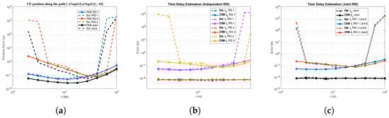
Figure 2. Single- and Multi-Ris NTN system: Estimation error and CRLB for (a) user position along $[-r/\sqrt{2},r/\sqrt{2},-10]$ with $r=[2,100]$ m, and (b,c) the corresponding time delay estimation.

4.2. Coverage Analysis

The coverage performance is evaluated using the Position Error Bound (PEB) across user positions $\mathbf{p}={[x,y,-5]}^{\top }$, with $x=-200\mathrm{to}-150$ m and $y=25\mathrm{to}500$ m, to identify areas meeting sub-meter accuracy. PEB is preferred over root mean square error (RMSE) for efficient large-area assessment, avoiding costly Monte Carlo simulations. Results in Figure 3 show PEB for single- and multi-RIS setups. With a single RIS, sub-meter accuracy is achieved near it, but errors rise up to 14 m at $y=500$ m. The multi-RIS setup extends sub-meter coverage to $175\times 100$ m² and limits maximum error to 7 m, significantly improving coverage and accuracy.

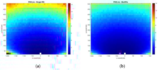
Figure 3. Coverage analysis for different user positions using PEB: (a) single-RIS configuration with RIS placed at ${[0,0,0]}^T$ (white square), and (b) multi-RIS configuration with RISs placed at ${[0,0,0]}^T$ (white square) and ${[-30,0,0]}^T$ (pink square).

5. Conclusions

This work has investigated the positioning performance of single- and multi-RIS configurations in an NTN system, focusing on estimation accuracy and coverage. By analyzing a diagonal user trajectory and computing the associated CRLB and estimation errors, we demonstrated that each individual RIS provides strong performance only within its localized region of influence. Specifically, RIS 1 is effective at low r values due to proximity, while RIS 2 becomes more relevant at larger distances. However, their individual performance degrades outside these optimal zones. In contrast, the multi-RIS configuration with joint processing consistently outperforms single-RIS setups across all regimes. It provides enhanced accuracy, especially in mid-range areas where neither individual RIS alone is dominant. It achieves an order-of-magnitude improvement in position estimation accuracy and closely tracks the CRLB. Furthermore, the coverage analysis confirms that the multi-RIS setup significantly extends the region where sub-meter accuracy is achieved by approximately $7\%$ and reduces average positioning error by about $20\%$. These gains validate the effectiveness of combining multiple RISs.

References

- Azari, M.M.; Solanki, S.; Chatzinotas, S.; Kodheli, O.; Sallouha, H.; Colpaert, A.; Montoya, J.F.M.; Pollin, S.; Haqiqatnejad, A.; Mostaani, A.; et al. Evolution of Non-Terrestrial Networks from 5G to 6G: A Survey. IEEE Commun. Surv. Tutor. 2022, 24, 2633–2672. [Google Scholar] [CrossRef]
- Luo, X.; Chen, H.H.; Guo, Q. LEO/VLEO Satellite Communications in 6G and Beyond Networks—Technologies, Applications and Challenges. IEEE Netw. 2024, 38, 273–285. [Google Scholar] [CrossRef]
- Reid, T.; Chan, B.; Goel, A.; Gunning, K.; Manning, B.; Martin, J. Satellite navigation for the age of autonomy. In Proceedings of the IEEE/ION PLANS, Portland, OR, USA, 23–26 April 2020; pp. 342–352. [Google Scholar]
- Fabra, F.; Egea–Roca, D.; López–Salcedo, J.A.; Seco–Granados, G. Analysis on signals for LEO-PNT beyond GNSS. In Proceedings of the 32nd European Signal Processing Conference (EUSIPCO), Lyon, France, 26–30 August 2024; IEEE: Piscataway, NJ, USA, 2024; pp. 1237–1241. [Google Scholar] [CrossRef]
- You, L.; Qiang, X.; Zhu, Y.; Jiang, F.; Tsinos, C.G.; Wang, W.; Wymeersch, H.; Gao, X.; Ottersten, B. Integrated communications and localization for massive MIMO LEO satellite systems. IEEE Trans. Wirel. Commun. 2024, 23, 11061–11075. [Google Scholar] [CrossRef]
- Wang, W.; Chen, T.; Ding, R.; Seco-Granados, G.; You, L.; Gao, X. Location-Based Timing Advance Estimation for 5G Integrated LEO Satellite Communications. IEEE Trans. Veh. Technol. 2021, 70, 6002–6017. [Google Scholar] [CrossRef]
- Saleh, S.; Keskin, M.F.; Priyanto, B.; Beale, M.; Zheng, P.; Al-Naffouri, T.Y.; Seco-Granados, G.; Wymeersch, H. 6G RIS-aided Single-LEO Localization with Slow and Fast Doppler Effects. In Proceedings of the GLOBECOM 2024, Cape Town, South Africa, 8–12 December 2024. [Google Scholar]
- Keykhosravi, K.; Keskin, M.F.; Seco-Granados, G.; Popovski, P.; Wymeersch, H. RIS-Enabled SISO localization under user mobility and spatial-wideband effects. IEEE J. Sel. Top. Signal Process. 2022, 16, 1125–1140. [Google Scholar] [CrossRef]
- Fadakar, A.; Sabbaghian, M.; Wymeersch, H. Multi-RIS-Assisted 3D localization and synchronization via deep learning. IEEE Open J. Commun. Soc. 2024, 5, 3299–3314. [Google Scholar] [CrossRef]
- Chen, H.; Zheng, P.; Keskin, M.F.; Al-Naffouri, T.; Wymeersch, H. Multi-RIS-Enabled 3D sidelink positioning. IEEE Trans. Wirel. Commun. 2024, 23, 8700–8716. [Google Scholar] [CrossRef]
- Keykhosravi, K.; Keskin, M.F.; Dwivedi, S.; Seco-Granados, G.; Wymeersch, H. Semi-Passive 3D positioning of multiple RIS-enabled users. IEEE Trans. Veh. Technol. 2021, 70, 11073–11077. [Google Scholar] [CrossRef]
- Wang, L.; Zheng, P.; Liu, X.; Ballal, T.; Al-Naffouri, T.Y. Beamgorming design and performance evaluation for RIS-aided localization using LEO satellite signals. In Proceedings of the ICASSP, IEEE International Conference on Acoustics, Speech and Signal Processing-Proceedings, Seoul, Republic of Korea, 14–19 April 2024; pp. 13166–13170. [Google Scholar] [CrossRef]
- Zheng, P.; Liu, X.; Al-Naffouri, T.Y. LEO- and RIS-empowered user tracking: A Riemannian manifold approach. IEEE J. Sel. Areas Commun. 2024, 42, 3445–3461. [Google Scholar] [CrossRef]
- Chen, H.; Sarieddeen, H.; Ballal, T.; Wymeersch, H.; Alouini, M.S.; Al-Naffouri, T.Y. A tutorial on Terahertz-band localization for 6G communication systems. IEEE Commun. Surv. Tutor. 2022, 24, 1780–1815. [Google Scholar] [CrossRef]
- Liu, X.; Ballal, T.; Chen, H.; Al-Naffouri, T.Y. Constrained wrapped least squares: A tool for high-accuracy GNSS attitude determination. IEEE Trans. Instrum. Meas. 2022, 71, 8005315. [Google Scholar] [CrossRef]
- Kaplan, E.; Hegarty, C. Understanding GPS: Principles and Applications, 2nd ed.; Artech House: London, UK, 2005. [Google Scholar]
Disclaimer/Publisher’s Note: The statements, opinions and data contained in all publications are solely those of the individual author(s) and contributor(s) and not of MDPI and/or the editor(s). MDPI and/or the editor(s) disclaim responsibility for any injury to people or property resulting from any ideas, methods, instructions or products referred to in the content. |
© 2026 by the authors. Licensee MDPI, Basel, Switzerland. This article is an open access article distributed under the terms and conditions of the Creative Commons Attribution (CC BY) license.