Abstract
A probabilistic–deterministic design of experiments (PDDoE) approach was employed to optimize laser-induced breakdown spectroscopy (LIBS) parameters for the quantitative determination of minor components in lead-based alloys. The PDDoE optimization identified 18 J laser pump lamp energy, 1 µs delay, and 1 µs exposure as optimal conditions, minimizing spectral dispersion (5–8%) and ensuring stable plasma formation. The acquired spectra were subsequently processed in an R-based automated workflow, where Linear, Lasso, and Ridge regression models were used to establish quantitative relationships between normalized line intensities and atomic absorption spectroscopy (AAS) reference data. The resulting models demonstrated high accuracy (R2 = 0.97 for Sn, 0.985 for Sb, 0.982 for Bi, 0.919 for As, and 0.905 for Ag), with prediction errors (RMSE) below 10% and limits of quantification (LOQ) under 0.05 wt.%. Principal component analysis (PCA) applied to 43 historical (19th–20th century) and technogenic samples (19th–20th century) allowed us to isolate clusters of Pb–Sb alloys corresponding to secondary accumulator materials, alongside a diffuse group of nearly pure Pb specimens containing variable minor impurities. The combined PDDoE–LIBS–R analytical framework provides a reproducible, non-destructive, and chemometrically validated methodology for the quantitative characterization and classification of archeological and industrial lead alloys.
Keywords:
LIBS; PDDoE; R workflow; lead alloys; regression models; PCA; chemometrics; archaeometallurgy; quantitative analysis 1. Introduction
While modern science continuously seeks safer alternatives to lead in everyday applications, lead alloy analysis remains relevant across numerous scientific and industrial fields. Laser-induced breakdown spectroscopy (LIBS) has emerged as a promising technique for such analysis, gaining popularity in contemporary analytical research. Lead is typically studied as an impurity [1] or contaminant in various media—soils [2], water [3], or archeological samples [4,5]; yet LIBS shows significant potential for analyzing lead-based materials themselves.
1.1. Application of LIBS in Analysis of Lead-Containing Objects
Although lead-based samples are not of much interest in current analytical studies, there are many studies focused on the identification and quantification of lead in different media, especially in the archeological field. Lead-containing archeological samples are actively studied using LIBS for trace element determination—Ag, Bi, Sn, Sb, and Cu. Studies have achieved remarkably low detection limits given sample composition complexity and matrix effects.
Tankova et al. showed that LIBS can assess Sn and Pb content in bronzes to draw conclusions about archeological metal artifact origins and manufacturing technology [4]. Penkova et al. analyzed bronze objects from the Late Bronze Age Baley settlement, constructing calibration dependencies using Pb/Cu line normalization that revealed Pb content differences among samples—interpreted as alloying for improved casting properties [5].
Both nanosecond and femtosecond LIBS have been applied to bronze alloy analysis, examining how pulse duration affects laser-induced plasma parameters and quantitative results for Sn, Zn, and Pb [6]. The method successfully analyzed three real metallic objects, with the results proving useful for future portable LIBS deployment for qualitative and quantitative elemental analysis of bronze artifacts in situ at museums and archeological sites.
Leonidova et al. explored the quantitative analysis of historical lead-silicate glasses by fusing calibration samples and building calibration curves for PbO and K2O [7]. Fomin et al. used LIBS for qualitative and quantitative analysis of lead enamels from the Jochi Khan Mausoleum (14th century) using thermodynamic and chemometric approaches [8].
Syvilay et al. investigated lead roof tiles from historical buildings, showing LIBS suitability for quantitative trace element determination (Ag, Bi, Cu, Sb, Sn) directly in a lead matrix, with LA-ICP-MS verification [9].
Fortes et al. developed a protocol for the rapid in situ identification of archaeometallurgical museum collections [10]. A novel mathematical algorithm enables rapid metallic artifact classification directly in museum settings.
Aside from archeology, LIBS application was shown to be successful in the analysis of industrial samples. LIBS combined with ICP-MS has proven successful for quantitative analysis and classification of Sn-Bi binary alloy solders, achieving 95–99% accuracy [11]. Calibration-free LIBS has also been used for the quantitative analysis of Pb-Sn binary alloys, with accuracy levels above 95% [12]. Comparing two CF-LIBS methods for Pb-Sn alloy quantification revealed that the electron density conservation method performs better than the Boltzmann plot approach for quantitative elemental analysis [13].
1.2. DOE and Chemometrics in LIBS Analysis
Spectral data quality suffers from numerous instrumental and environmental influences, making preliminary experimental design crucial for any study. This matters particularly in LIBS, where spectral lines undergo matrix effects in the process of analysis of complex samples. Design of experiments serves as a universal tool applicable to various sample types for obtaining data with maximum informativity [14,15].
Applying design of experiments to the multi-elemental analysis of river sediments showed that fractional factorial design and central composite design (CCD) effectively optimize the key parameters affecting complex sample analysis by LIBS [16].
Improving result reproducibility represents another important LIBS analysis task. Autofocus systems ensuring consistent lens-to-sample distance in each experiment significantly reduce spectral standard deviation and improve reproducibility [17]. This matters especially when analyzing samples with varying surface flatness.
Proper normalization of spectral data is also crucial in LIBS analysis. A detailed study on the impact of the reference-line choice under non-LTE conditions was reported [18], highlighting that the ratio stability strongly depends on ΔE between transitions.
Probabilistic-deterministic design of experiments (PDDoE) offers a promising factorial analysis method. Unlike one-factor optimization, it evaluates both individual and combined factor influences. This method has shown potential for analyzing various samples—archeological artifacts (including lead-containing ones), coal tar, and other complex composition objects [10,19,20].
Various signal enhancement modes improve signal quality and analytical sensitivity. Triple-pulse LIBS, combining pre-ablation and reheating pulses, can provide up to 5-fold signal-to-background improvement versus double-pulse configurations and up to 228-fold improvement versus conventional single-pulse LIBS [21].
Achieving optimal results also requires modern data post-processing methods. Chemometric methods are widely used in LIBS analysis for the extraction of useful information from large arrays of complex spectral data [22,23,24]. The most popular include principal component analysis (PCA), multiple linear regression (MLR), and partial least squares (PLS/PLS-R). Chemometric methods based on artificial neural networks have also gained recent popularity [25].
Partial least squares (PLS) combined with support vector regression (SVR) and random forest (RF) achieved accurate coal quality analysis using a portable LIBS device, with mean relative error of 2.19% for volatile matter determination [26]. Various chemometric methods were compared for quantitative heavy metal content analysis in soils, including Cd and Pb [27].
Successful LIBS analysis of complex lead alloys requires a dual approach: experimental parameters (via design of experiments and multi-pulse excitation) to ensure high-quality signals, and chemometric processing (regularized regression and multivariate methods) to compensate for matrix effects and maximize analytical accuracy. This combined approach can potentially be useful in enabling robust quantification and classification in challenging lead-based matrices.
1.3. Specific Considerations for Lead Alloy Analysis
Despite these advances, quantitative LIBS analysis of lead-based alloys remains challenging due to matrix effects, self-absorption, surface heterogeneity, and shot-to-shot variations. Successful implementation requires systematic optimization of instrumental parameters, appropriate normalization strategies to compensate for matrix effects, and robust calibration approaches. While design of experiments (DoE) methodologies have proven effective for parameter optimization in various LIBS applications, their application to archeological lead alloys—which often exhibit complex, variable matrices and surface corrosion—remains limited.
In this work, we present a systematic approach to the LIBS quantification of minor elements (Sn, Sb, Bi, Ag, As, Au) in historical lead-based alloys. The study combines: (1) probabilistic-deterministic design of experiments for instrumental parameter optimization; (2) double-pulse excitation for enhanced sensitivity; (3) element-specific normalization strategies selected through iterative evaluation; and (4) regularized regression models (Lasso, Ridge) to address multicollinearity in spectral data. Method performance was validated through comparison with atomic absorption spectroscopy measurements on archeological samples from Central Kazakhstan.
2. Materials and Methods
2.1. Preparation of Calibration Lead Alloy Standards
Metallic Pb granules (99.9% purity) served as the base for all calibration alloys. Prior to alloy preparation, real lead-based samples were collected and qualitatively analyzed to identify typical impurity elements. Based on this analysis, seven metals were selected as alloying components: Sn, Sb, Bi, Ag, As, and Au (all 99.9% purity). The absence of significant impurities in starting materials was confirmed by LIBS. Metal concentrations were selected based on expected impurity ranges in real lead samples, with the total additive concentration in each alloy set at 10 wt%.
Alloys were prepared by induction melting in corundum crucibles with flux. The flux consisted of ethanol rosin solution (10% concentration) and a 50:50 mixture of magnesium chloride and potassium chloride powders. The melting procedure was as follows:
- 1.
- Bi, Sn, and Sb were dissolved in half the Pb mass at 700 °C for 30 min with constant stirring;
- 2.
- Ag and Au were dissolved in the remaining Pb at 800 °C for 30 min;
- 3.
- The resulting metal solutions were combined and thoroughly mixed at 700–800 °C for 15 min;
- 4.
- The resulting alloy was cooled to 400–450 °C, then the As was added, while continuously stirring the metal solution;
- 5.
- The melt was cooled to room temperature using an air stream directly in the crucible.
The final alloy compositions were verified by atomic absorption spectroscopy (AAS). Table 1 contains the concentrations of the added elements in the primary calibration set.

Table 1.
Added component concentrations in calibration set verified by AAS.
To extend the calibration range, diluted alloys were prepared by mixing the primary standards with pure lead. Five dilution series were created with component concentrations reduced by factors of 2, 4, 6, 8, and 16. Each subsequent dilution set was prepared by twofold dilution of the previous set with pure Pb. Component concentrations in all diluted samples were verified by AAS.
All alloys were polished and checked for homogeneity by comparing emission spectra registered from upper and lower surfaces, as well as from different locations across the sample cross-section.
2.2. Analytical and Sample Preparation Devices
LIBS measurements were performed using a MATRIX CONTINUUM LIBS device (“Spectroscopic Systems”, Moscow, Russia) equipped with a Nd:YAG solid-state laser with double pulse configuration operating at 1064 nm. The instrumental specifications, according to manufacturer documentation, are a maximum pulse energy of 100 mJ per pulse, and an average of 60 mJ (at a laser pump lamp energy of 16 J). The duration of the laser pulse is non-variable and is up to 10–15 ns, the diameter of the laser beam is up to 4 mm, and the electric energy of the laser lamp pump is up to 35 J, with a working range of 12–20 J.
The detection system employs a Czerny-Turner optical configuration with dual spectrograph channels (focal lengths 250 mm and 125 mm) equipped with diffraction gratings (2400 lines/mm and 1200 lines/mm, respectively) and seven CCD detectors (“Toshiba”, Tokyo, Japan; TCD1304DG model with 3648 pixels each). Five of the detectors cover 170–408 nm (wavelength sampling ~0.013 nm/pixel, spectral resolution ~0.03–0.05 nm FWHM), while two detectors span 408–800 nm (sampling ~0.05 nm/pixel, resolution ~0.1–0.15 nm FWHM). This configuration prioritizes high resolution in the 170–408 nm range. The present study utilized the high-resolution 170–408 nm range.
Sample surfaces were positioned using an automated XYZ stage with a video monitoring system. For each measurement point, multiple laser pulses were applied, with spectra averaged to improve signal-to-noise ratio. All measurements were conducted in air at atmospheric pressure and room temperature.
Validation of the components’ concentration was conducted on atomic absorption spectrometer “Varian AA 140”.
To ensure the smooth and flat surface of the calibration and real samples, a grinding machine with sandpaper of various grits and polishing pastes were used.
All metallography pictures were taken with trinocular inverted metallurgical microscope (“Hualong”, Shanghai, China; HL102-BW model) with a 10× objective lens. Prior to metallography, the polished sample surface was etched by H2O2:CH3COOH = 1:3 (by volume).
2.3. Experimental Design for Parameter Optimization
2.3.1. Probabilistic-Deterministic Design of Experiments
Optimal LIBS analysis device parameters were determined using probabilistic-deterministic design of experiments (PDDoE) [28,29]. PDDoE is a multifactorial optimization method enabling simultaneous evaluation of parameter effects on experimental outcomes. Unlike sequential one-factor-at-a-time approaches, PDDoE reduces experimental time by systematically varying all factors concurrently according to a balanced design, where each level of each factor is combined with each level of every other factor exactly once. The method extracts individual response curves (partial functions) for each factor by averaging experimental outcomes across all trials sharing the same factor level; this balanced structure ensures that effects of other factors cancel out during averaging. The partial functions are then algebraically approximated and combined into a multiplicative predictive model. This yields mathematical relationships between response variables (e.g., normalized line intensity, reproducibility) and individual factors or their interactions.
The employed design examined 6 factors at 5 levels, requiring 25 measurements at unique conditions.
The optimization procedure included: (1) selection of instrumental parameters as optimization factors; (2) definition of parameter variation ranges where effects were expected to be most significant; (3) construction of an experimental matrix with a balanced structure: 6 factors at 5 levels in 25 experiments using Latin hypercube design, where each factor level appears exactly 5 times; (4) extraction of partial dependences by averaging responses for experiments with identical factor levels (5 measurements per level); (5) algebraic fitting of partial functions using appropriate curves (linear, parabolic, etc.) based on visual inspection and physical expectations; (6) statistical validation of factor significance using correlation coefficients.
The optimization was focused on the enhancement of normalized line intensities and reproducibility (expressed as relative standard deviation from 5 replicates) for selected analytical lines. Line assignments were verified against the NIST Atomic Spectra Database [30]. Au and As lines were excluded from the optimization process due to their initially low or undetectable signal intensities. However, the optimization of instrumental parameters based on other elements was expected to enhance overall spectral intensity, potentially making these lines detectable and suitable for subsequent model training.
Five instrumental parameters were systematically varied: laser pump lamp energy, QSW1 timing (the delay between the flashlamp triggering and the Q-switch opening, which affects pulse energy and temporal characteristics), inter-pulse delay ΔQSW (the time interval between the first and second laser pulse in the double-pulse configuration), detection delay (the time between the second laser pulse and spectral acquisition onset), and integration time (the charge accumulation period controlled by the ICG electronic shutter). Direct control of the laser pulse energy was not available on the instrument, although the energy is measured internally; therefore, pump lamp energy was used as the optimization variable. A sixth factor—analyte concentration—was included in the design matrix by rotating calibration samples between experiments (one sample per five experiments) and served primarily as a verification factor to confirm the expected linear relationship between concentration and signal intensity. Table 2 presents the optimization factors and their variation levels. Factors 2–6 represent instrumental parameters with levels corresponding to different device settings. Factor 1 (concentration, C%) was varied by rotating calibration standards with different analyte concentrations, serving as a verification parameter to confirm the expected concentration-intensity relationship.
Table 2.
Chosen PDDoE optimization factors (LIBS device settings) and their levels.
The laser frequency and number of laser shots per point were fixed throughout the experiment and were 6 Hz and 20 shots, accordingly. Experiments were performed on five calibration samples, with the complete set of experiments replicated five times to obtain sufficient statistical sampling.
2.3.2. Spectral Normalization
To eliminate uncontrolled experimental variations, spectral normalization was performed prior to optimization experiment calculations. A medium-intensity lead line without visible self-absorption—Pb 401.96 nm—served as the internal standard. For the optimization experiments, normalization by a single reference line was sufficient to evaluate relative changes in signal intensity and reproducibility across different instrumental parameters. This simplified approach allowed efficient assessment of parameter effects without introducing additional complexity while maintaining the time efficiency, which is a key advantage of PDDoE. For each set of five replicates, outliers were identified and removed using Dixon’s Q-test. Subsequently, normalized intensities (the analyte line intensity divided by the Pb 401.96 intensity) were calculated, and mean values with standard deviations were determined for each experimental condition.
This normalization strategy compensates for shot-to-shot laser energy fluctuations, plasma instabilities, and variations in sample positioning. Table 3 illustrates the normalization procedure with data for the Sn 284.00 nm line (sample 1 of the calibration set).
Table 3.
Example of spectral data processing algorithm for optimization experiment.
It should be noted that the normalization strategies differed between the optimization and calibration stages: simplified single-line normalization was used for parameter optimization, while element-specific normalization was employed for quantitative calibration (detailed in Section 2.4.5).
2.4. Calibration Model Development
2.4.1. Data Collection
LIBS spectra were acquired from 30 calibration standards under the optimized instrumental parameters determined. Five replicate measurements per sample were collected at different surface locations, yielding 150 total spectra for model development.
2.4.2. Data Import and Preprocessing
Data processing was performed in R (v. 4.5.2) [31] using packages vroom (v. 1.6.7), tidyverse (v. 2.0.0), openxlsx (v. 4.2.8.1), ggplot2 (v. 4.0.1), and plotly (v.4.11.0) for data manipulation, analysis, and visualization. Each spectrum was assigned a unique identifier derived from the filename. All data were combined into a single long-format table, then transformed into a matrix (wide format) where rows corresponded to individual spectra and columns to fixed wavelengths.
The combined spectrum was constructed, where maximum intensity at each wavelength across all spectra was retained, preserving even weak lines present only in specific samples. This approach proved superior to summed or averaged spectra, where weak lines could be lost against intense background emission.
2.4.3. Peak Detection and Line Selection
Analytical lines were identified from the combined spectrum. An adaptive noise threshold was calculated to enable weak peak detection while suppressing random fluctuations. The threshold was defined as half of the maximum value between the mean and median baseline intensity. In the composite spectrum, the mean intensity slightly exceeded the median due to the presence of numerous weak emission lines, indicating a positively skewed intensity distribution. Taking the maximum of these two values ensured a conservative threshold that retained genuine weak peaks while filtering noise.
Peaks were identified through local maximum screening: a point was recognized as a peak if its intensity exceeded the threshold and it lay within a monotonically increasing-then-decreasing region. To prevent duplicate detection of closely spaced maxima, a minimum wavelength spacing of 0.015 nm (comparable to the instrumental resolution) was enforced.
For each individual spectrum, local maxima were then sought within ±0.015 nm windows around identified peak positions, generating an intensity matrix for all samples and all detected lines.
2.4.4. Training Dataset Construction
Reference element concentrations in calibration standards were imported from Excel files using the openxlsx R package. To avoid division by zero in subsequent calculations, zero concentrations were replaced with a nominal minimum value (10−6). Peak intensity data and concentration data were merged based on sample identifiers. Normalized intensities were calculated to further reduce instrumental drift effects.
2.4.5. Spectral Normalization Approach
Normalization is critical in LIBS analysis to compensate for shot-to-shot variations in laser energy, plasma conditions, and matrix effects. While single-line normalization (Pb I 401.96 nm) was used during parameter optimization for computational efficiency, a systematic approach was employed to identify optimal normalization lines for the quantitative calibration of each element.
All detected Pb emission lines [N = 12] across the spectral range were evaluated as potential normalization references. For each target element (Sn, Sb, Bi, As, Ag), the following iterative procedure was applied:
- (1)
- Analyte line intensities were normalized by dividing by the intensity of each Pb line individually, generating N normalization variants.
- (2)
- For each normalization variant, three regression model types (multilinear regression, Lasso, Ridge) were trained on the calibration dataset.
- (3)
- Model performance was evaluated using coefficient of determination (R2) and root mean square error (RMSE) on a validation subset.
- (4)
- The Pb normalization line yielding the highest average R2 and lowest RMSE across all three model types was selected as the optimal reference for that element.
This element-specific optimization accounts for differences in excitation conditions, transition probabilities, and ionization energies between analyte and reference lines, thereby minimizing systematic errors and improving calibration accuracy. The selected optimal normalization lines for each element are reported in Section 3.3.
2.4.6. Model Training, Validation, and Performance Metrics
Three regression approaches were implemented for each element: multilinear regression (MLR), Lasso regression (L1 regularization), and Ridge regression (L2 regularization). Models were trained on the complete calibration dataset consisting of 30 standard samples with known elemental compositions.
Internal model performance was assessed using coefficient of determination (R2), root mean square error (RMSE), and mean absolute error (MAE) calculated through leave-one-out cross-validation (LOOCV) on the calibration standards. This approach evaluates model stability and identifies potential overfitting without requiring a separate validation subset from the limited calibration data.
External validation was performed using 15 archeological lead-based samples as an independent test set. Reference concentrations for these samples were determined by atomic absorption spectroscopy (AAS), and LIBS predictions were compared against AAS measurements to assess real-world analytical performance. Predicted versus measured concentration plots were generated for both calibration standards and archeological samples, with equality lines and confidence intervals to visualize accuracy and identify systematic deviations.
2.5. Prediction of Unknown Sample Compositions
Best-performing models were applied to spectra from unknown samples (identified by prefix Unk_). In total, the study included 43 unknown samples, from which 2 samples initially identified as lead-based but subsequently determined to be Zn- and Sn-based alloys were excluded, and 15 used as a control set for the trained models.
Five replicate LIBS measurements for each unknown sample improved prediction reliability. Predicted values underwent two-stage outlier filtering using Dixon’s Q-test, effectively removing spurious results, even with small replicate numbers (3–7 measurements).
The final results for each unknown sample included mean predicted concentrations, standard deviations, 95% confidence intervals, and numbers of replicates retained after filtering. Results were automatically saved to Excel files with separate sheets for each model family (Linear, Lasso, Ridge).
2.6. Multivariate Analysis
Principal component analysis (PCA) was performed on predicted concentrations of minor elements (Sn, Sb, Bi, Ag, As, Au) using the prcomp function in R. Pb was not included as a PCA variable since it constitutes the matrix element present at >90% in all samples, providing minimal discriminatory information.
Data were centered and scaled before PCA. The first three principal components typically captured approximately 90% of total variance.
PCA results were visualized in two-dimensional space (PC2 vs. PC3) using biplot representation (ggplot2 package), where both sample scores and variable loadings were overlaid on a single plot. This visualization enabled simultaneous assessment of sample similarities and identification of the compositional variables (minor elements) driving the observed groupings. Samples clustering in biplot space indicated similar compositional profiles, with cluster positions determined by the dominant alloying element(s). This approach facilitated the rapid evaluation of predicted composition plausibility and identification of compositional patterns among archeological artifacts.
2.7. Determination of Detection and Quantification Limits
Limits of detection (LOD) and quantification (LOQ) were calculated following IUPAC recommendations [32] and contemporary refinements [33,34]. For each Lasso regression model describing the relationship between element concentration and normalized line intensities, the slope S and standard error σ were determined. Parameter S represents effective model sensitivity (Euclidean norm of coefficient vector β), while σ characterizes residual dispersion of predicted versus certified concentrations.
Detection and quantification limits were calculated using classical relationships:
LOD = 3.3 × σ/S
LOQ = 10 × σ/S
The parameter σ encompasses noise from the entire analytical procedure, including plasma variability, laser fluctuations, and normalization uncertainties, while S represents the model response to unit concentration change. Thus, the obtained LOD/LOQ values reflect both statistical and physicochemical limitations of LIBS analysis.
Pure Pb spectra acquired under identical excitation conditions served as the blank matrix. For elements present as alloying additions (Sb, Bi, Sn, Ag, As), Lasso regression automatically excluded irrelevant lines, ensuring linearity in the low-concentration range and robustness against multicollinearity. For gold (Au), ordinary linear regression without regularization was applied due to the limited number of suitable training peaks.
3. Results and Discussion
This section presents results from laser parameter optimization, spectral collection, and regression model development for quantitative determination of components in lead alloys by LIBS. The work focuses on the experimental identification of conditions ensuring maximum signal reproducibility, minimum dispersion, and physically plausible relationships between analytical line intensities and element concentrations.
Device setting optimization established conditions under which stable laser-induced plasma clouds form, while acquired spectra exhibit good repeatability and sufficient excitation levels. Based on these data, linear and regularized regression models (Lasso, Ridge) were constructed, enabling accurate concentration determination even in complex Pb matrices.
3.1. Laser Parameter Optimization
Probabilistic-deterministic design of experiments (PDDoE) revealed consistent physicochemical patterns during the laser ablation of lead alloys. Among investigated instrumental factors—laser pump lamp energy, Q-switch parameters (QSW1 and ΔQSW), delay, and exposure time—laser pump lamp energy demonstrated the greatest influence on signal characteristics.
Optimization was primarily guided by the Sn 284.00 nm line behavior, as this line showed the most pronounced response to parameter variations. Other analytical lines showed similar optimization trends but with lower sensitivity to parameter changes, likely due to effective normalization reducing matrix effects and instrumental variations for these elements. Increasing energy from 12 to 20 J reduced the relative standard deviation of normalized line intensities: Figure 1 shows the dependency of dispersion (coefficient of variation, CoV) on laser pump lamp energy for Sn 284.00 spectral line. The five data points represent averaged CoV values calculated from all experiments (5 replicates each) performed at the same lamp pump energy level. The solid blue line represents the algebraic approximation obtained by fitting a linear function to these five points using the least squares method. The red dashed horizontal line indicates the overall mean CoV across all 25 experiments, serving as a baseline for assessing factor influence. The approximation quality is characterized by the coefficient of nonlinear multiple correlation (R). The significance criterion (tR) tests whether the correlation is statistically meaningful; values tR > 2 indicate significant factor influence at 95% confidence level. For this partial function, R = 0.8868 and tR = 7.1914, confirming that pump lamp energy significantly affects measurement reproducibility.
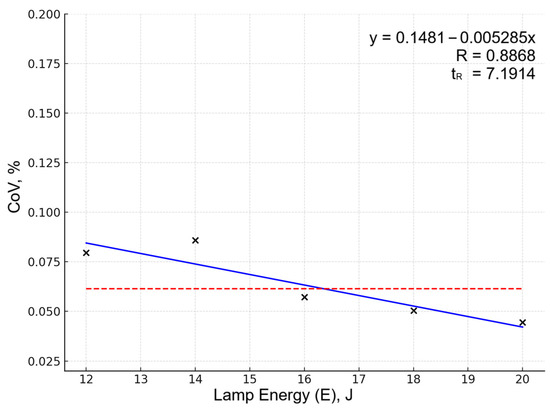
Figure 1.
Dependency of CoV on lamp energy for the Sn 284.00 spectral line. Data points (×) represent averaged CoV values (5 experiments per pump lamp energy level). Blue line shows linear approximation; red dashed line indicates overall mean CoV serving as baseline.
This is the result of the more complete vaporization of microscopic volumes and enhanced plasma homogeneity, reducing the influence of alloy microstructural inhomogeneities. Increasing exposure time above 3 μs caused more result scatter, associated with capturing late plasma stages when recombination processes are dominant and excitation temperature decreases. During this period, minor element signals weaken while noise components grow, lessening signal-to-noise ratios.
Alloying element line intensities (Sn, Sb, Bi, Ag) decreased at high energy despite better reproducibility (Figure 2 shows an example of this on the same Sn 284.00 line). This is explained by self-absorption effects and plasma shielding: enhanced Pb matrix emission reduces the relative contribution of weak lines. Such behavior is characteristic of lead systems under excessive material evaporation.
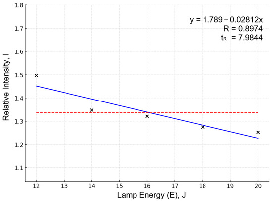
Figure 2.
Dependency of relative intensity (I) on lamp energy for the Sn284.00 spectral line. Data points (×) represent averaged relative intensity (I) values (5 experiments per pump lamp energy level). Blue line shows linear approximation; red dashed line indicates overall mean I serving as baseline.
Optimal parameters providing a compromise between stability and signal intensity were established as follows:
- Laser energy: 18 J
- QSW1: 101 μs
- ΔQSW: 3 μs
- Delay: 1 μs
- Exposure: 1 µs
Under the optimal conditions, the laser system delivered double pulses with energies of approximately 60 mJ (first pulse, Channel 1) and 70 mJ (second pulse, Channel 2), as measured by the instrument’s built-in energy monitoring system.
Since QSW1 timing, inter-pulse delay (ΔQSW), and detection delay did not significantly affect the normalized line intensities or measurement reproducibility, these parameters were held constant at empirically determined values that ensured stable instrumental performance.
The optimized parameter combination was validated by comparing predicted and experimentally measured normalized intensities across five calibration standards. As an example, for the Sn284.00 line, for a highest concentration standard (Sample 3), the response surface model predicted a normalized intensity of 1.14, while verification measurements yielded 1.103 ± 0.041 (n = 5), representing a 3.2% deviation from the prediction. Validation across the full calibration range showed an average deviation of <4% between predicted and measured intensities.
Measurement reproducibility improved with increasing Sn concentration: the relative standard deviation ranged from 14.5% at the lowest concentration to 3.7–3.9% at mid-to-high concentrations, consistent with the expected signal-to-noise behavior in spectroscopic analysis. This concentration-dependent precision demonstrates that the optimized conditions provide good reproducibility within the practical working range while maintaining acceptable performance near quantification limits.
3.2. Spectral Collection Under Optimal Conditions
After determination of the optimal device settings (Energy = 18 J, QSW1 = 101 μs, ΔQSW = 3 μs, Delay = 1 μs, Exposure = 1 µs), a series of spectra accumulation in the optimal parameters were performed on all sample sets—calibration, control, and unknown. Each measurement was performed five times, enabling the assessment of signal reproducibility and plasma stability under selected settings.
Spectral data were processed using custom R scripts. Individual spectra were combined into a data matrix, and a composite reference spectrum was created by taking the maximum intensity at each wavelength across all measurements, thereby preserving weak lines that might be present in only some samples.
Peak detection proceeded as follows: (1) local maxima were identified in the composite spectrum; (2) baseline mean and median intensities were calculated; (3) peaks below half the mean intensity were rejected as noise; (4) for each retained peak wavelength, intensities were extracted from individual spectra by searching for local maxima within ±0.015 nm windows (corresponding to instrumental resolution). The result was an intensity matrix for all samples and detected lines.
Extracted peak positions were used to construct an intensity matrix presented in file tbl_peaks.xlsx. Each row corresponds to an individual spectrum (with the sample and repetition number), while each column represents the wavelength of a registered peak. Thus, the table contains complete measurement descriptions, including training and control samples as well as “unknown” spectra with prefix Unk_.
Replicate analysis (n = 5) showed that signal reproducibility substantially improved under optimized conditions. For the Sn I 284.00 nm line (used as the primary optimization target), the relative standard deviation (RSD) decreased from 5 to 8% after optimization. Post-optimization measurements of calibration standards confirmed that other main analytical lines (Sb I 287.79 nm, Bi I 289.80 nm, Ag I 328.07 nm) exhibited similar reproducibility (RSD 5–10%), indicating that optimization based on Sn effectively improved performance across all target elements. The improved reproducibility demonstrates the successful stabilization of ablation and plasma formation through the optimized parameter combination.
Notably, spatial surface inhomogeneity of samples (especially in diluted alloys) did not lead to noticeable changes in spectral profiles, indicating uniform impurity distribution throughout alloy volumes and confirming the correctness of calibration material preparation methods.
The obtained tbl_peaks.xlsx table thus represents a reproducible, statistically stable base of spectral features suitable for further quantitative model construction and analysis of linear and regularized dependencies between intensities and component concentrations.
3.3. Metallographic Characterization of Calibration Alloys
Metallographic examination of calibration samples showed that all alloys possess fine-grained Pb matrix structures with uniformly distributed alloying component inclusions (Figure 3). Sb, Bi, and Sn impurities form isometric inclusions of rounded or elongated shape, ranging from 5 to 30 μm, are uniformly distributed throughout sample volumes. Silver and arsenic inclusions occur less frequently and predominantly localize along grain boundaries.
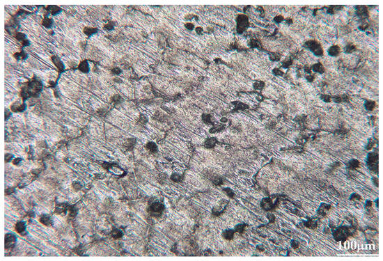
Figure 3.
Metallographic picture of one of the calibration alloys (10× optical zoom).
The absence of segregation zones and pronounced enrichment regions indicates good alloy homogenization during preparation. At typical LIBS crater diameters (80–120 μm), each laser pulse encompasses several such inclusions simultaneously, providing averaging over local inhomogeneity and enhancing signal reproducibility (Figure 4 and Figure 5). This is consistent with the observed intensity dispersion reduction under optimal ablation parameters (σ = 5–8%).
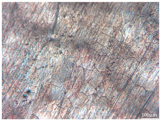
Figure 4.
Metallographic picture of one of the unknown samples (sample #26) (10× optical zoom).
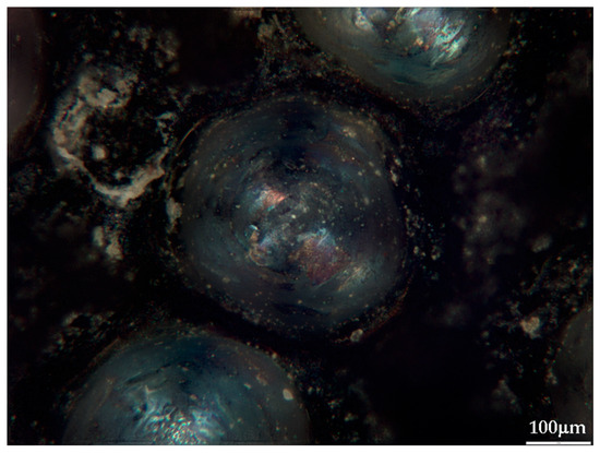
Figure 5.
Picolay [35] focus-picking photo of a crater, left after analysis (sample #26) (10× optical zoom).
Microstructural homogeneity and size correspondence between inclusions and crater diameter ensure measurement representativeness and confirm the correctness of using prepared alloys as calibration standards.
3.4. Regression Model Development and Analysis
Three model types were constructed for quantitative spectral data interpretation—multiple linear regression (LM), Lasso, and Ridge regression—each using normalized analytical line intensities divided by the selected Pb line intensity (internal standard).
General Equation Form
For all the elements, equations took the form of the following function:
where Ii is the i-th line intensity of the given element, IPb,k is the normalizing Pb line intensity, βi are weight coefficients determined by regression, and ε is random error.
For Lasso and Ridge models, standard regularization criteria were used:
where Y is the vector of observed response values (measured element concentrations, n × 1), X is the matrix of predictors (normalized line intensities, n × p), β is the vector of model coefficients (p × 1), ‖Y − Xβ‖22 is the residual sum of squares (RSS), λ is the regularization parameter (λ ≥ 0) controlling the penalty strength, ‖β‖1 is the L1-norm (sum of absolute values, promoting sparsity in Lasso), and ‖β‖22 is the squared L2-norm (sum of squared coefficients, shrinking but not eliminating parameters in Ridge).
Multiple Linear Models (LM)
For most elements, 10 to 35 analytical lines were used, reflecting the complex nature of plasma spectra and the need to account for both strong and moderate transitions.
For example, for Sn in the model normalized by Pb 265.7 nm, the equation obtained was:
with R2 = 0.9715 coefficient of determination.
The most significant predictors were lines Sn 284.01, 285.05, 281.26, 303.28, 270.65, 278.49 nm, possessing stable linear response. Such high correlation reflects a linear intensity increase with concentration, typical for elements with moderate excitation energies (4–5 eV) under relatively cold Pb plasma conditions.
For antimony (Sb) in the model normalized by Pb 401.96 nm, 20 lines were used, including Sb 204.96, 217.92, 236.04, 237.38, 276.98, 287.79, 323.25, 326.75 nm, with R2 = 0.985 (Figure 6). The multiple lines here result from a strong Sb line overlap with Pb and Sn lines, requiring several independent combinations for reliable modeling.
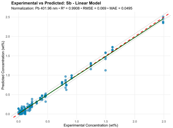
Figure 6.
Graphic representation of the linear regression model for the Sb element.
In the graphs, a dashed red line denotes an ideal 1:1 relationship, a solid green line denotes a fitted trend, and dashed black lines denote the ± RMSE prediction interval. High result consistency indicates effective model performance even under significant multicollinearity.
Lasso Regression
L1-norm regularization eliminated the least significant or correlated lines, while the number of retained peaks remained substantial—10–20 per element.
For Sb under identical conditions, Lasso excluded the weak lines (e.g., 222.06 nm, 302.98 nm) but retained the main lines: 204.96, 236.04, 237.38, 267.06, 276.98, 287.79, 323.25, 326.75 nm, with a slight R2 decrease (0.9838 versus 0.985). For Sn, there was a similar effect—a model with 30 lines and R2 = 0.968 provided slightly lower accuracy but better cross-validation stability (Figure 7).
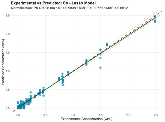
Figure 7.
Graphic representation of the lasso model for the Sb element.
Lasso eliminates noisy and overlapping lines while preserving physically meaningful dependencies. This model proves especially useful for weak intensity or partial line overlap (e.g., Sn 303.28 and 303.42 nm).
Ridge Regression
Ridge models showed the greatest robustness to multicollinearity, which is important for dense Pb matrix spectra.
For example, for bismuth (Bi) normalized by Pb 257.74 nm, the model included 11 lines (213.36–351.07 nm) and achieved R2 = 0.9824 (Figure 8).
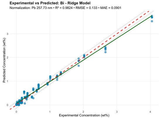
Figure 8.
Graphic representation of the ridge model for the Bi element.
Despite line proximity and strong correlations, Ridge preserved all predictors by “shrinking” their weights and preventing overfitting. Visually, the predictions agreed well with the experimental concentrations (RMSE < 5%), confirming the normalization method and line selection correctness. A comparison of the methods is shown in Table 4 and Figure 9.
Table 4.
Comparison of applied regression approaches.
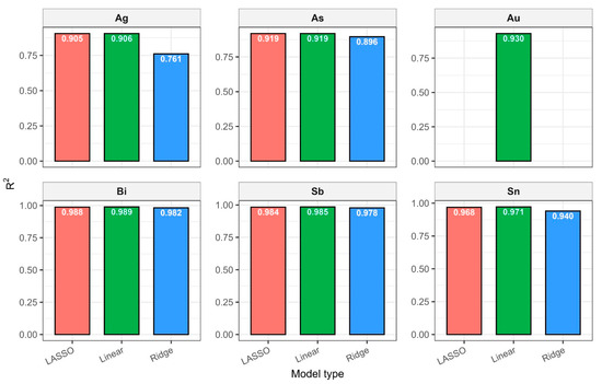
Figure 9.
Comparison of regression models for each element.
Physicochemical Interpretation
The presence of dozens of stable lines for Sn, Sb, and Bi indicates that even in lead matrices, a wide plasma temperature zone persists, enabling excitation of both low-energy and medium-energy transitions.
Regularization analysis revealed that spectral lines of minor elements exhibit correlated responses to plasma parameter variations driven by the lead matrix composition. Multiple lines of the same element respond coherently to shot-to-shot fluctuations in plasma temperature and electron density, as these conditions are primarily determined by the dominant matrix composition. The regularized models (Lasso, Ridge) exploit this correlation structure by weighting ensembles of co-varying lines rather than selecting single features, thereby improving prediction robustness through redundancy and reducing sensitivity to individual line measurement errors. Lines consistently assigned high coefficients across all model types (e.g., Sn I 281.35 nm, Sb I 287.79 nm, Bi I 302.46 nm) can be considered the most stable analytical indicators for future method development.
Optimal regression models thus describe alloying element concentration dependencies in Pb alloys with high accuracy (R2 > 0.9 in all cases) and demonstrate physical validity: linearity across working concentration ranges and a predictable influence of lines with varying excitation potentials.
3.5. Model Validation
To assess quantitative element determination reliability by LIBS, calibration results (LIBS wt%) were compared with control values measured by atomic absorption spectroscopy (AAS wt%). Regression dependencies and statistical indicators (R2, RMSE, and Bias) were calculated for 15 control samples covering wide alloying component concentration ranges.
Summary data are provided in table LIBS_vs_AAS_stats.xlsx. The mean determination coefficients for all elements exceeded 0.9, indicating high linear agreement between LIBS results and reference values. The best agreement was observed for Sn and Sn (R2 = 0.985 and 0.971, respectively), related to the stable and saturated lines of these elements in spectra. For bismuth and arsenic, R2 values remained above 0.95, though slight negative Bias was observed, associated with the partial self-absorption of intense lines at elevated concentrations. The most noticeable discrepancy (R2 approx. 0.90, RMSE around 0.02–0.03 wt%) was recorded for silver, where spectral lines possess low intensity and partially overlap with Pb lines.
Systematic deviations (Bias) for all elements did not exceed 0.05 wt% in absolute units, corresponding to typical LIBS method uncertainty for metallic matrices. No noticeable concentration-dependent deviation sign was observed—deviations were random in nature, indicating the absence of systematic calibration error. High R2 values with moderate RMSE and small Bias confirm method consistency and normalizing Pb line selection correctness.
On constructed LIBS vs. AAS plots for the main components of the samples (Figure 10, Figure 11, Figure 12 and Figure 13), all points lie along the equality line without pronounced deviation trends. This confirms model chemical plausibility: predicted Sn, Sb, Bi, and As contents correspond to the expected ranges for lead alloys, while absent impurities show no false-positive signals. Visual slight range compression for Bi and As represents a typical compensation effect in multidimensional regression with high variable correlation. In the graphs, a dashed black line denotes the ideal 1:1 relationship and a solid red line denotes the fitted trend.
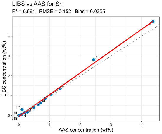
Figure 10.
LIBS vs. AAS Sn quantitative analysis results comparison.
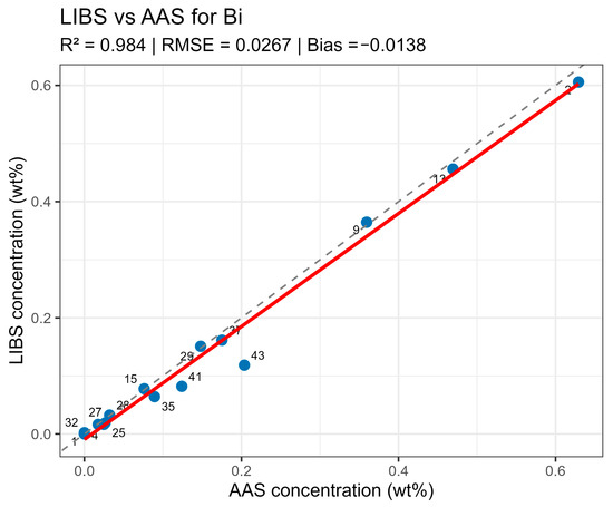
Figure 11.
LIBS vs. AAS Bi quantitative analysis results comparison.
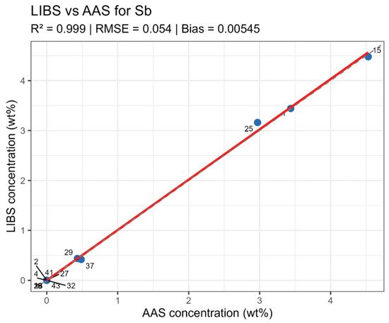
Figure 12.
LIBS vs. AAS Sb quantitative analysis results comparison.
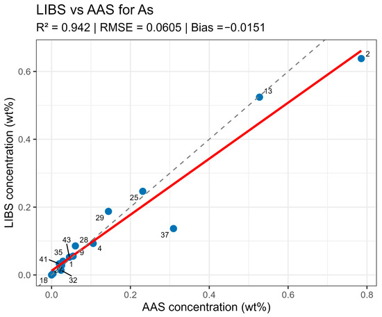
Figure 13.
LIBS vs. AAS As quantitative analysis results comparison.
Control sample verification thus demonstrated that the constructed LIBS models ensure correct concentration recovery in real matrices. The method exhibited high accuracy with minimal systematic deviations and fully reproducible results upon repeated measurements, enabling its application for the quantitative analysis of “unknown” alloys with similar matrix composition.
3.6. PCA of Analysis Results
Principal component analysis (PCA) was performed to compare the compositional profiles of the lead-based alloys using concentrations of five minor elements: bismuth (Bi), antimony (Sb), arsenic (As), silver (Ag), and tin (Sn). Samples with non-lead matrices were excluded from the analysis, resulting in a dataset of 41 observations. Gold (Au), as previously mentioned, was not included in the final variable set due to its low concentration and irregular occurrence in archeological samples.
The sample set consists of archeological and technogenic lead-based artifacts collected during field expeditions in Central Kazakhstan. Archeological objects include metallurgical waste from non-ferrous metal smelting and refining operations (the earliest specimen tentatively dated to a 19th-century smelter based on stratigraphic context), and fragments of decorative items and tools. Technogenic samples comprise battery grids, fishing sinkers, seals, and structural lead components, predominantly from the late 19th through 20th centuries based on archeological context and typology. Representative samples are shown in Figure 14; a complete catalog of all analyzed samples is provided in the Supplementary Materials. All are characterized by lead matrix (Pb content exceeding 90 wt%), with total alloying additions not exceeding 6 wt%.
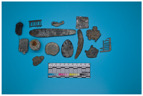
Figure 14.
Some of the analyzed archeological and industrial samples.
LIBS spectra from archeological samples were acquired under the previously determined optimized instrumental conditions. Five replicate measurements were performed at different locations on each sample to account for surface heterogeneity.
Element concentrations were predicted using the optimal calibration models, with intensities normalized using the same Pb reference lines as employed during model training. The resulting predicted concentration matrix (41 samples × 5 elements) served as the input for principal component analysis.
In addition to the quantified minor elements, the alloys contain other trace impurities (Cu, Zn, etc.) that were not explicitly determined. Lead concentration was not directly measured; however, it is inherently anti-correlated with the sum of quantified minor element concentrations (Pb ≈ 100% − ∑minor elements). Consequently, lead was excluded from PCA as it would provide redundant information without enhancing compositional discrimination among samples.
The first principal component (PC1) primarily reflects Bi content with additional contribution from Ag. The second component (PC2) is predominantly determined by Sb with partial influence from As. The third component (PC3) is associated with the Sb-Bi ratio, enabling identification of technological differences in alloy compositions.
The biplot (Figure 15) reveals clear grouping based on bismuth and antimony content: alloys with high Bi are displaced along PC1, while Sb-enriched alloys occupy the opposite region of the plot. Samples with elevated Sn content form a distinct subgroup with positive PC3 values, potentially indicating the use of secondary remelting or different raw material sources.
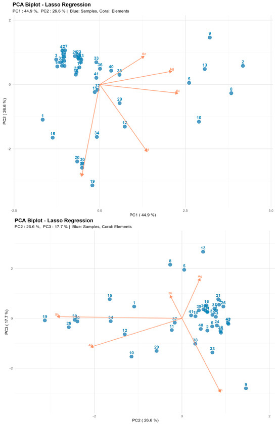
Figure 15.
Results of PCA on unknown samples.
This separation has both physicochemical and historical-technological foundations. While the lead matrix maintains homogeneity across all groups, the observed differences reflect deliberate alloying choices, the evolution of metallurgical processes, and varying levels of ore refining across different periods. Clustering based on Sb, Bi, As, and Ag effectively captures the technological evolution from minimally refined early systems to standardized battery-grade materials. The PCA results demonstrate that LIBS can serve not only for quantitative compositional analysis but also as a tool for identifying historical-technological groups among archeological metal artifacts. The observed differentiation of principal components is consistent with archeological context data and indicates the potential for the technological classification of finds based on elemental profiles. This approach offers a rapid, minimally destructive method for the preliminary sorting and characterization of large archeological assemblages prior to more detailed analyses.
4. Conclusions
The conducted experimental series showed that laser source device setting optimization substantially improves LIBS analysis reproducibility for lead alloys. At a laser pump lamp energy of 18 J, a delay of 1 μs, and an exposure of 1 μs, minimum signal dispersion (standard deviation 5–8%) is achieved while maintaining sufficient analytical line intensity. Such conditions ensure stable plasma formation and an adequate balance between impurity element excitation and Pb matrix emission.
Regression models (Linear, Lasso, Ridge) showed high agreement with experimental data. Determination coefficients for the key elements were: Sn—0.97, Sb—0.985, Bi—0.982, As—0.919, and Ag—0.905. Quantification limits (LOQ) did not exceed 0.05 wt% even for elements with low line intensity. Root mean square prediction error (RMSE) for control samples remained within 7–10%, while mean deviation (Bias) did not exceed 0.05 wt%. These results confirm the possibility of the reliable quantitative analysis of Pb-Sb-Sn-Bi-As system alloys without complex sample preparation. Au content in all the samples was lower than the LOD, so for its quantification, further research development is required.
Comparison with atomic absorption analysis (AAS) confirmed the model’s adequacy: the mean R2 for the control samples exceeded 0.9, the RMSE did not exceed 0.03 wt%, and the Bias was random in nature. The LIBS method with correct Pb line normalization thus provides analytical accuracy comparable to laboratory reference methods and can be applied for rapid alloy identification.
Principal component analysis (PCA) revealed three stable groups: Pb-Sb battery alloys (late 20th century), Pb-Bi technical alloys (mid-20th century), and Pb-As-Ag systems from the late 19th to early 20th century. Principal components PC1, PC2, and PC3 explain approximately 95% of variance, confirming the statistical significance of the discovered classification and its correspondence to historical-technological alloy evolution.
Supplementary Materials
The following supporting information can be downloaded at: https://www.mdpi.com/article/10.3390/analytica6040055/s1, ZIP Archive “Spectra.zip”: spectra of all the samples (*.txt format)—calibration and unknown—registred in calculated optimal condition; ZIP Archive “Lead_photos”: photos of all the studied unknown and calibration samples; defineAAS.xlsx: results of AAS analysis of test samples set; EN_Scripts.docx: pipeline of scripts used for spectra processing; Small_database.xlsx: necessary information on lines of the elements investigated in the research (Kurucz); spectra_with_peaks.png and tbl_peaks.xlsx: WL of researched analytical lines derived by the scripts.
Author Contributions
Conceptualization, V.F.; methodology, M.T.; software, V.F.; validation, M.T., N.A. and S.A.; formal analysis, S.A.; investigation, A.A.; resources, D.S.; data curation, D.K.; writing—original draft preparation, N.K.; writing—review and editing, M.T.; visualization, A.B.; supervision, V.F.; project administration, V.F. All authors have read and agreed to the published version of the manuscript.
Funding
This research was funded by the Science Committee of the Ministry of Science and Higher Education of the Republic of Kazakhstan (Grant No. AP19677716 «Development of methods for qualitative and quantitative analysis of lead and copper alloys using laser induced breakdown spectroscopy and chemometrics»).
Data Availability Statement
Data is contained within the article or Supplementary Material.
Conflicts of Interest
The authors declare no conflicts of interest. The funders had no role in the design of the study; in the collection, analyses, or interpretation of data; in the writing of the manuscript; or in the decision to publish the results.
Abbreviations
The following abbreviations are used in this manuscript:
| LIBS | Laser Induced Breakdown Spectroscopy |
| PDDoE | Probabilistic-deterministic design of experiments |
| Q-SW | Q-Switch |
| AAS | Atomic Absorbtion Spectroscopy |
| LoD | Limit of Detection |
| LoQ | Limit of Quantification |
| CoV | Coefficient of Variation |
| LM | Linear Model |
| RMSE | Root Mean Square Error |
| MAE | Mean Absolute Error |
| LOOCV | Leave-One-Out Cross Validation |
| PCA | Principal Component Analysis |
References
- Zhang, Y.; Zhang, T.; Li, H. Application of laser-induced breakdown spectroscopy (LIBS) in environmental monitoring. Spectrochim. Acta Part B At. Spectrosc. 2021, 181, 106218. [Google Scholar] [CrossRef]
- Kim, G.; Kwak, J.; Kim, K.-R.; Lee, H.; Kim, K.-W.; Yang, H.; Park, K. Rapid detection of soils contaminated with heavy metals and oils by laser induced breakdown spectroscopy (LIBS). J. Hazard. Mater. 2013, 263, 754–760. [Google Scholar] [CrossRef]
- Schlatter, N.; Lottermoser, B.G. Laser-Induced Breakdown Spectroscopy Applied to Elemental Analysis of Aqueous Solutions—A Comprehensive Review. Spectrosc. J. 2024, 2, 1–32. [Google Scholar] [CrossRef]
- Tankova, V.; Malcheva, G.; Blagoev, K.; Leshtakov, L. Investigation of archaeological metal artefacts by laser-induced breakdown spectroscopy (LIBS). J. Phys. Conf. Ser. 2018, 992, 012003. [Google Scholar] [CrossRef]
- Penkova, P.; Malcheva, G.; Grozeva, M.; Hristova, T.; Ivanov, G.; Alexandrov, S.; Blagoev, K.; Tankova, V.; Mihailov, V. Laser-Induced Breakdown Spectroscopy and X-ray Fluorescence Analysis of Bronze Objects from the Late Bronze Age Baley Settlement, Bulgaria. Quantum Beam Sci. 2023, 7, 22. [Google Scholar] [CrossRef]
- Elhassan, A.; Giakoumaki, A.; Anglos, D.; Ingo, G.M.; Robbiola, L.; Harith, M.A. Nanosecond and femtosecond Laser Induced Breakdown Spectroscopic analysis of bronze alloys. Spectrochim. Acta Part B At. Spectrosc. 2008, 63, 504–511. [Google Scholar] [CrossRef]
- Leonidova, A.; Aseev, V.; Prokuratov, D.; Jolshin, D.; Khodasevich, M. Application of Laser-Induced Breakdown Spectroscopy for Quantitative Analysis of the Chemical Composition of Historical Lead Silicate Glasses. Quantum Beam Sci. 2023, 7, 24. [Google Scholar] [CrossRef]
- Fomin, V.N.; Usmanova, E.R.; Gyul, E.F.; Kelesbek, N.K.; Turovets, M.A.; Zemskiy, O.I.; Saulebekov, D.M.; Aldabergenova, S.K. Method for Qualitative and Quantitative Analysis of Ancient Lead Enamel Using Laser Induced Breakdown Spectroscopy. Bull. Univ. Karaganda Chem. 2022, 108, 16–27. [Google Scholar]
- Syvilay, D.; Texier, A.; Arles, A.; Gratuze, B.; Wilkie-Chancellier, N.; Martinez, L.; Serfaty, S.; Detalle, V. Trace element quantification of lead based roof sheets of historical monuments by LIBS. Spectrochim. Acta Part B At. Spectrosc. 2015, 103–104, 34–42. [Google Scholar] [CrossRef]
- Fortes, F.J.; Cabalín, L.M.; Laserna, J.J. Fast and in-situ identification of archaeometallurgical collections in the museum of Malaga using laser-induced breakdown spectroscopy and a new mathematical algorithm. Heritage 2020, 3, 1330–1343. [Google Scholar] [CrossRef]
- Galbács, G.; Jedlinszki, N.; Metzinger, A. Analysis and discrimination of soldering tin samples by collinear multi-pulse laser induced breakdown spectrometry, supported by inductively coupled plasma optical emission and mass spectrometry. Microchem. J. 2013, 107, 17–24. [Google Scholar] [CrossRef]
- Urbina, I.; Carneiro, D.; Rocha, S.; Farias, E.E.; Bredice, F.; Palleschi, V. Study of binary lead-tin alloys using a new procedure based on calibration-free laser induced breakdown spectroscopy. Spectrochim. Acta Part B At. Spectrosc. 2020, 170, 105902. [Google Scholar] [CrossRef]
- Najarian, M.; Chinni, R. Temperature and Electron Density Determination on Laser-Induced Breakdown Spectroscopy (LIBS) Plasmas: A Physical Chemistry Experiment. J. Chem. Educ. 2013, 90, 244–247. [Google Scholar] [CrossRef]
- Cioccia, G.; Pereira de Morais, C.; Babos, D.V.; Milori, D.M.B.P.; Alves, C.Z.; Cena, C.; Nicolodelli, G.; Marangoni, B.S. Laser-Induced Breakdown Spectroscopy Associated with the Design of Experiments and Machine Learning for Discrimination of Brachiaria brizantha Seed Vigor. Sensors 2022, 22, 5067. [Google Scholar] [CrossRef] [PubMed]
- Shaw, G.; Martin, M.Z.; Martin, R.; Biewer, T.M. Preliminary design of laser-induced breakdown spectroscopy for proto-Material Plasma Exposure eXperiment. Rev. Sci. Instrum. 2014, 85, 11D806. [Google Scholar] [CrossRef]
- Pereira de Morais, C.; Nicolodelli, G.; Mitsuyuki, M.C.; Mounier, S.; Milori, D.M.B.P. Optimization of laser-induced breakdown spectroscopy parameters from the design of experiments for multi-element qualitative analysis in river sediment. Spectrochim. Acta Part B At. Spectrosc. 2021, 177, 106066. [Google Scholar] [CrossRef]
- Chide, B.; Maurice, S.; Murdoch, N.; Lasue, J.; Bousquet, B.; Jacob, X.; Cousin, A.; Forni, O.; Gasnault, O.; Meslin, P.-Y.; et al. Listening to laser sparks: A link between Laser-Induced Breakdown Spectroscopy, acoustic measurements and crater morphology. Spectrochim. Acta Part B At. Spectrosc. 2019, 153, 50–64. [Google Scholar] [CrossRef]
- Lazic, V.; Fantoni, R.; Falzone, S.; Gioia, P.; Loreti, E.M. Stratigraphic Characterization of Ancient Roman Frescos by Laser Induced Breakdown Spectroscopy and Importance of a Proper Choice of the Normalizing Lines. Spectrochim. Acta Part B At. Spectrosc. 2020, 168, 105853. [Google Scholar] [CrossRef]
- Turovets, M.A.; Fomin, V.N.; Kelesbek, N.K.; Kaykenov, D.A.; Sadyrbekov, D.T.; Aynabayev, A.A.; Aldabergenova, S.K. Chemometric Approach for the Determination of Vanadium by the LIBS Method. Eurasian J. Chem. 2024, 116, 61–70. [Google Scholar] [CrossRef]
- Fomin, V.N.; Aynabaev, A.A.; Kaykenov, D.A.; Sadyrbekov, D.T.; Aldabergenova, S.K.; Turovets, M.A.; Kelesbek, N.K. Optimization of coal tar gas chromatography conditions using probabilistic-deterministic design of experiment. Bull. Univ. Karaganda Chem. 2021, 104, 39–46. [Google Scholar] [CrossRef]
- Prochazka, D.; Pořízka, P.; Novotny, J.; Hrdlička, A.; Novotný, K.; Šperka, P.; Kaiser, J. Triple-pulse LIBS: Laser-induced breakdown spectroscopy signal enhancement by combination of pre-ablation and re-heating laser pulses. J. Anal. At. Spectrom. 2020, 35, 603–612. [Google Scholar] [CrossRef]
- Wang, H.-P.; Chen, P.; Dai, J.-W.; Liu, D.; Li, J.-Y.; Xu, Y.; Chu, X. Recent advances of chemometric calibration methods in modern spectroscopy: Algorithms, strategy, and related issues. TrAC Trends Anal. Chem. 2022, 153, 116648. [Google Scholar] [CrossRef]
- Zhang, T.; Tang, H.; Li, H. Chemometrics in laser-induced breakdown spectroscopy: Progress of Chemometrics in Laser-induced Breakdown Spectroscopy. J. Chemom. 2018, 32, e2983. [Google Scholar] [CrossRef]
- Zhang, T.-L.; Wu, S.; Tang, H.-S.; Wang, K.; Duan, Y.-X.; Li, H. Progress of Chemometrics in Laser-induced Breakdown Spectroscopy Analysis. Chin. J. Anal. Chem. 2015, 43, 939–948. [Google Scholar] [CrossRef]
- Li, L.-N.; Liu, X.-F.; Yang, F.; Xu, W.-M.; Wang, J.-Y.; Shu, R. A review of artificial neural network based chemometrics applied in laser-induced breakdown spectroscopy analysis. Spectrochim. Acta Part B At. Spectrosc. 2021, 180, 106183. [Google Scholar] [CrossRef]
- Dou, Y.; Wang, Q.; Wang, S.; Shu, X.; Ni, M.; Li, Y. Quantitative Analysis of Coal Quality by a Portable Laser Induced Breakdown Spectroscopy and Three Chemometrics Methods. Appl. Sci. 2023, 13, 10049. [Google Scholar] [CrossRef]
- Adhikari, N.; Martyshkin, D.; Fedorov, V.; Das, D.; Antony, V.; Mirov, S. Laser-Induced Breakdown Spectroscopy Detection of Heavy Metal Contamination in Soil Samples from North Birmingham, Alabama. Appl. Sci. 2024, 14, 7868. [Google Scholar] [CrossRef]
- Malyshev, V.P. Veroyatnostno-Determinirivannoe Planirovanie Eksperimenta; Nauka: Almaty, Kazakhstan, 1981. [Google Scholar]
- Fomin, V.N.; Aldabergenova, S.K.; Rustembekov, K.T.; Omarov, K.B.; Rozhkovoy, I.E.; Dik, A.V.; Saulebekov, D.M. Optimization of the Parameters of a Laser Induced Breakdown Spectrometer (LIBS) Using Probabilistic-Deterministic Design of Experiment. Ind. Lab. Diagn. Mater. 2021, 87, 14–19. [Google Scholar] [CrossRef]
- NIST Atomic Spectra Database. Available online: https://www.nist.gov/pml/atomic-spectra-database (accessed on 15 October 2025).
- R Core Team. R: A Language and Environment for Statistical Computing; R Foundation for Statistical Computing: Vienna, Austria, 2025; Available online: https://www.R-project.org/ (accessed on 15 October 2025).
- Currie, L.A. Nomenclature in evaluation of analytical methods including detection and quantification capabilities. Pure Appl. Chem. 1995, 67, 1699–1723. [Google Scholar] [CrossRef]
- Gegenschatz, T.; Kononenko, T.; Pedarnig, J.D. Multivariate methods for calibration and limit of detection determination in LIBS. Anal. Chim. Acta 2021, 1180, 338899. [Google Scholar]
- Pedarnig, J.D.; Sturm, V.; Rachbauer, R. Review of Element Analysis of Industrial Materials by LIBS. Appl. Sci. 2021, 11, 9274. [Google Scholar] [CrossRef]
- PICOLAY—Focus Stacking Software. Available online: https://www.picolay.de/ (accessed on 15 October 2025).


Disclaimer/Publisher’s Note: The statements, opinions and data contained in all publications are solely those of the individual author(s) and contributor(s) and not of MDPI and/or the editor(s). MDPI and/or the editor(s) disclaim responsibility for any injury to people or property resulting from any ideas, methods, instructions or products referred to in the content. |
© 2025 by the authors. Licensee MDPI, Basel, Switzerland. This article is an open access article distributed under the terms and conditions of the Creative Commons Attribution (CC BY) license (https://creativecommons.org/licenses/by/4.0/).