Effective and Efficient Resonant Transitions in Periodically Modulated Quantum Systems

Abstract

We analyze periodically modulated quantum systems with $SU\left(2\right)$ and $SU(1,1)$ symmetries. Transforming the Hamiltonian into the Floquet representation we apply the Lie transformation method, which allows us to classify all effective resonant transitions emerging in time-dependent systems. In the case of a single periodically perturbed system, we propose an explicit iterative procedure for the determination of the effective interaction constants corresponding to every resonance both for weak and strong modulation. For coupled quantum systems we determine the efficient resonant transitions appearing as a result of time modulation and intrinsic non-linearities.

1. Introduction

Effective transitions in time-dependent quantum systems have been extensively studied since the classical paper [1], later generalized in [2,3], and widely applied for the description of atomic dynamics in external fields [4,5,6,7,8,9,10,11,12,13,14,15,16] and in more involved periodically perturbed quantum systems [17,18,19,20,21,22,23]. Effective transitions are described by operators that: (i) Become time-independent (resonant) in an appropriate reference frame under certain relations between the system’s frequencies (resonant conditions); (ii) are not present in the original Hamiltonian; and (iii) disappear in the rotating wave approximation (RWA). Such resonant terms (later referred to as resonances) naturally appear in the effective Hamiltonian in the weak interaction limit where the counter-rotating (CR) contributions, rapidly oscillating in any reference frame terms, are perturbatively taken into account. The most famous examples of time-dependent systems with an infinite number of effective resonances are the Rabi model in classical field [1,2,3] and the parametric quantum oscillator [24]. Even in these simplest systems, where the Hamiltonian is a linear form on the $SU\left(2\right)$ and $SU(1,1)$ Lie algebras, it turns out that the general expressions for the effective interaction constants and the frequency shifts in the vicinity of each resonance, are not easy to obtain.

The situation becomes even more complicated when two coupled quantum systems are subjected to time-dependent periodic perturbations e.g., as in the quantum Rabi model with modulated coupling and/or frequency. In these types of models, CR terms (in the absence of external fields) are responsible for several physical effects such as: Multiphoton atom-field interactions in the Rabi model [25,26], an improvement of a qubit photodetector readout [27], the excitation of several atoms by a single photon [25,28], and several other effective processes now experimentally achievable in solid state circuit quantum electrodynamics (QED) setups [29,30,31,32]. An additional periodic excitation makes the situation even richer, leading to e.g., the enhancement of CR interactions in the Rabi model [16], the generation of specific non-classical photon states [17], the emergence of non-linear spin-boson couplings [18], the appearance of quantum to classical phase-transitions [19], lasing with a single atom [20], simulation of the anisotropic Rabi model [21], or the dynamical Casimir effect [22].

One of the possibilities to construct a perturbation theory that unveils the effective resonant interactions, is the Lie transformation method [33,34]. Such a method consists in order-by-order elimination of CR terms by a specific set of transformations, whose particular form directly follows from the algebraic structure of the original Hamiltonian [25]. The advantage of this approach consists in a rather simple and systematic procedure for obtaining the general form of effective resonance terms and the order of the corresponding effective coupling constants.

The aim of the present paper is to provide a systematic approach to the analysis of effective resonant transitions in quantum systems obeying the $SU\left(2\right)$, $SU(1,1)$, and $H\left(1\right)$ symmetries with periodically modulated frequencies and/or coupling constants. We construct the Lie-type all-order perturbation theory allowing to determine the order of every possible resonance that may emerge in the effective Hamiltonians. We consider both single and coupled quantum systems and determine the efficient resonant transitions emerging as a combination of the time modulation and intrinsic non-linearities, especially relevant in interacting systems.

In Section 2 we outline the Lie transformation method in an example of a single periodically perturbed $SU\left(2\right)$/$SU(1,1)$ system and provide not only the order of the effective resonance terms [35] but the explicit iterative procedure for determining the effective interaction constants both for the weak and strong modulation. In Section 3 we analyze coupled time-dependent quantum systems and discuss types of efficient resonances proper to different symmetries of the interacting systems.

2. Single Periodically Modulated Quantum System

2.1. General Settings

Let us consider a quantum system described by the following time-dependent Hamiltonian (the case where only the frequency of the system is modulated is considered in Section 2.4),

$$H_{\pm }\left(t\right)=\omega X_0+2g_{0}cos\left(\nu t\right)X_0+2g_{1}cos\left(\nu t\right)\left(X_{+}+X_{-}\right),\omega ,\nu >0,$$

(1)

where the operators $X_{\pm },X_0$, satisfy the following commutation relations:

$$\left[X_0,X_{\pm }\right]=\pm X_{\pm },\left[X_{+},X_{-}\right]=\pm 2X_0,$$

(2)

the signs ± correspond to the $SU\left(2\right)$ and $SU(1,1)$ algebras respectively. In the interaction picture the Hamiltonian takes the form:

$$\begin{array}{}\mathrm{(3)}& \hfill H_{int\pm }\left(t\right)& =& g_0\left(e^{i\nu t}+e^{-i\nu t}\right)X_0\hfill \mathrm{(4)}& & & +g_1\left(e^{i(\omega +\nu )t}{X}_{+}+e^{i(\omega -\nu )t}{X}_{+}+h.c.\right),\hfill \end{array}$$

where the terms $\sim e^{i(\omega -\nu )t}{X}_{+}+h.c.$ become time independent if $\omega =\nu$ and correspond to the principal resonance, while the counter-rotating (CR) terms $\sim cos\left(\nu t\right)X_0$ and $e^{i(\omega +\nu )t}{X}_{+}+h.c.$ rapidly oscillate for any relation between the frequencies.

The CR terms are neglected in the zero-order approximation when $g_1\sim g_0\ll \omega ,\nu$ (RWA) and the Hamiltonian (3) and (4) acquires a simple form:

$$H_{int\pm }\approx g_1\left(e^{i(\omega -\nu )t}{X}_{+}+h.c.\right).$$

In the opposite limit, $g_1\ll g_0\sim \omega ,\nu$ the zero-order approximation gives the diagonal Hamiltonian:

$$H_{int\pm }\approx g_0\left(e^{i\nu t}+e^{-i\nu t}\right)X_0,$$

characterized by a trivial dynamics. The CR terms in (3) and (4) lead to the emergence of non-trivial resonant transitions, not explicitly present in the original Hamiltonian. It is well known that in the case of $H\left(1\right)$ symmetry, $X_{+}=a^{†},X_{-}=a$, $X_0=a^{†}a$, no resonances additional to the principal one $\sim a{e}^{i(\omega -\nu )t}$ appear.

In order to develop the Lie-perturbation theory that allows to describe all possible effective resonances both in the limits $g_{0,1}\ll \omega ,\nu$ and $g_1\ll g_0\sim \omega ,\nu$, we introduce the Euclidean algebra operators $E,E^{†},E_0$, obeying the commutation relations:

$$[E_0,E]=-E,[E_0,E^{†}]=E^{†},[E^{†},E]=0,$$

(5)

where $E^{†}E=E{E}^{†}=I$. Then, the Hamiltonian (1) can be put in a one-to-one correspondence with the following time-independent (Floquet) form [35]:

$$\begin{array}{ccc}\hfill H_{\pm }^F& =& \omega X_0+\nu E_0+g_0\left(E+E^{†}\right)X_0\hfill \\ & & +g_1\left(E+E^{†}\right)\left(X_{+}+X_{-}\right),\hfill \end{array}$$

(6)

where the Euclidean operators $(E,E^{†},E_0)$ describe a “classical” field interacting with the X-system. The time-dependent Hamiltonian (1) is recovered from (4) by transforming it to the frame rotating with the “classical frequency” $\nu$,

$$\begin{array}{ccc}\hfill H_{int\pm }^F& =& g_0\left(e^{i\nu t}{E}^{†}+e^{-i\nu t}E\right)X_0\hfill \\ & & +g_1\left(e^{it\left(\omega +\nu \right)}{E}^{†}{X}_{+}+e^{it\left(\omega -\nu \right)}E{X}_{+}+h.c.\right),\hfill \end{array}$$

with a subsequent averaging over the eigenstates of $E,E^{†}$ operators (phase-states), $E\left|\varphi \right.⟩=e^{-i\varphi }\left|\varphi \right.⟩$,

$$\left|\varphi \right.⟩=\underset{N\to \infty }{lim}\frac{1}{\sqrt{2N+1}}\sum _{n=-N}^N{e}^{-in\varphi }\left|n\right.⟩,$$

(7)

where $E_0\left|n\right.⟩=n\left|n\right.⟩$, and setting the initial phase $\varphi =0$ without loss of generality. The CR terms are now identified with $\sim \left(E+E^{†}\right)X_0$ and $\sim \left(E{X}_{-}+E^{†}{X}_{+}\right)$.

2.2. Effective Hamiltonian, $g_{0,1}\ll \omega ,\nu$

We start with the most complicated limit $g_0\sim g_1\ll \omega ,\nu$, when the contributions of diagonal and non-diagonal CR terms in (3) and (4) are of the same order. The CR terms appearing in the Floquet Hamiltonian (6) can be removed order-by-order by applying a set of Lie-type transformations according to the general scheme [25,33,34] as shown in Appendix A.

The common feature of all of these transformations (small rotations) is their form:

$$V_k=e^{{\epsilon }_k\left(Z_{+}^{\left(k\right)}-Z_{-}^{\left(k\right)}\right)},$$

(8)

where ${\epsilon }_k\ll 1$ are some appropriate small parameters, under the condition that the Hamiltonian, which is transformed by (8), should contain the term $Z_0^{\left(k\right)}$ such that $\left[Z_0^{\left(k\right)},Z_{\pm }^{\left(k\right)}\right]=\pm Z_{\pm }^{\left(k\right)}$. The resonance expansion is obtained as a power series of the small parameters ${\epsilon }_k$ and only contains terms that become time-independent in appropriate reference frames.

The resulting resonance expansion in the leading order in each effective coupling constant $g_1{ϵ}_{\pm k}$ has the form:

$$H_{RE\pm }^F\approx \tilde{\omega }{X}_0+\nu E_0+g_1\sum _{k=0}^{\infty }{ϵ}_{\pm k}\left(E^{k+1}{X}_{+}+E^{k+1}{X}_{-}\right),$$

(9)

where $\tilde{\omega }$ is a modified X-system frequency, ${ϵ}_{\pm 0}=1$,

$${ϵ}_{\pm k}=\frac{{\mathrm{B}}_k\left(a_{\pm 1},a_{\pm 2},\dots ,a_{\pm k}\right)}{k!},$$

(10)

where:

$$a_{\pm k}=-{\nu }^{-1}(k-1)!h_{\pm k},$$

and ${\mathrm{B}}_k\left(a_{\pm 1},a_{\pm 2},\dots ,a_{\pm k}\right)$ are the complete Bell polynomials [36], and the constants $h_{\pm k}$ are obtained recursively according to $h_{\pm 1}=g_0$, $h_{\pm 2}=\pm 2g_1^2/\left(\omega +\nu \right)$ and:

$$\begin{array}{ccc}\hfill h_{\pm (2k+2)}& =& -\frac{h_{\pm (k+1)}^2}{2\left(\omega +(2k+1)\nu \right)}\hfill \\ & & -\frac{1}{\omega +(2k+1)\nu }\sum _{m=1}^k{h}_{\pm m}{h}_{\pm (2k+2-m)},\hfill \end{array}$$

(11)

$$\begin{array}{ccc}\hfill h_{\pm (2k+1)}& =& -\frac{1}{\omega +2k\nu }\sum _{m=1}^k{h}_{\pm m}{h}_{\pm (2k+1-m)},\hfill \end{array}$$

(12)

for $k=1,\dots$. One can appreciate that ${ϵ}_{\pm k}$ is a k-th order homogeneous polynomial ${\epsilon }^{\left(k\right)}$ (A5) on some small parameters $\epsilon \sim g_{0,1}/l.c.(\omega ,\nu )\ll 1$, where $l.c.(\omega ,\nu )$ represents non zero linear combinations of $\omega$ and $\nu$ for any relation between the frequencies.

The resonance expansion (9) contains all possible effective resonant transitions that may emerge in (6) and indicates that such transitions happen only at $(k+1)\nu =\tilde{\omega }$, where the case $k=0$ corresponds to the principal resonance present in the original Hamiltonian.

In principle, the effective Hamiltonian, describing the system excitation in the vicinity of every particular resonance, should still be obtained from the resonance expansion (9) by removing all of the other resonances. However, as is proven in Appendix A, the elimination of all terms in (9) that become non-resonant under the condition $\omega \approx (k+1)\nu$ does not change the leading order of the effective interaction constants $g_1{ϵ}_{\pm k}$, thus the effective Hamiltonian has the form:

$$\begin{array}{ccc}\hfill H_{\pm (k+1)}^F& \approx & {\tilde{\omega }}_{\pm (k+1)}{X}_0+\nu E_0\hfill \\ & & +g_1{ϵ}_{\pm k}\left(E^{k+1}{X}_{+}+E^{†k+1}{X}_{-}\right).\hfill \end{array}$$

(13)

The effective X-system frequency ${\tilde{\omega }}_{\pm (k+1)}$ includes small shifts that should be taken into account up to the order of the coupling constant $g_1{ϵ}_{\pm k}$, which determines the width of the corresponding resonance.

The evolution operator corresponding to the effective Hamiltonian (13) under the resonance condition ${\tilde{\omega }}_{\pm (k+1)}=(k+1)\nu$ is:

$$U_{\pm }^F\left(t\right)=e^{-i\nu t\left((k+1)X_0+E_0\right)}{e}^{-it{g}_1{ϵ}_{\pm k}\left(E^{k+1}{X}_{+}+E^{†k+1}{X}_{-}\right)},$$

(14)

and can be disentangled in the standard way. Using (14), the evolution of any observable can be computed without returning to the time-dependent frame. This is achieved by transforming the corresponding X-system operator with (14) and averaging the result over the phase states (7). Strictly speaking, the evolution operator should still be transformed with all the transformations of the form (8) used for removing non-resonant terms in order to obtain the effective Hamiltonian (13). Nevertheless, since the transformations (8) are time independent, they lead only to small modifications of amplitudes and can be neglected in the first approximation. For instance, the evolution of $X_0$ operator in the resonance ${\tilde{\omega }}_{\pm (k+1)}=(k+1)\nu$ can be easily found using (14),

$$X_0\left(t\right)=X_{0}C\left(2t{g}_1{ϵ}_{\pm k}\right)+\frac{i}{2}\left(X_{-}-X_{+}\right)S\left(2t{g}_1{ϵ}_{\pm k}\right),$$

where $C\left(x\right)=cos\left(x\right)$, $S\left(x\right)=sin\left(x\right)$ for the $su\left(2\right)$ algebra and $C\left(x\right)=cosh\left(x\right)$, $S\left(x\right)=sinh\left(x\right)$ for the $SU(1,1)$ algebra.

The frequency shifts for the lowest resonances can be easily found by a direct application of the transformations given in Appendix A. In order to obtain ${\tilde{\omega }}_{\pm (k+1)}$ for the highest order resonances the following procedure can be applied: The effective Hamiltonian (13) is unitary equivalent to (6) up to k-th order on some small parameters. In other words there exists a unitary transformation of the form:

$$O_{\pm }=exp\left\{({\alpha }_{\pm }^{†}-{\alpha }_{\pm })X_0+{\beta }_{\pm }{X}_{+}-{\beta }_{\pm }^{†}{X}_{-}\right\},$$

(15)

where

$${\alpha }_{\pm }\left(E\right)=\sum _{j=1}{a}_{\pm j}{E}^j,{\beta }_{\pm }(E,E^{†})=\sum _{j=0}{b}_{\pm j}{E}^j+c_{\pm j}{E}^{†j},$$

(16)

such that under the condition $\omega \approx (k+1)\nu$:

$$O_{\pm }^{†}{H}^F{O}_{\pm }=H_{\pm (k+1)}+\mathcal{O}\left({\epsilon }^{(k+1)}\right).$$

Taking into account the form of the perturbative action of transformations of the type (15) on the Hamiltonian (6), as discussed in Appendix A, we realize that every coefficient in (16) can be expanded in a series on some small parameters to be determined:

$$x_{\pm j}=\sum _m{x}_{\pm j}^{\left(m\right)},x_{\pm j}^{\left(m\right)}\sim {\epsilon }^{(j+2m)},$$

(17)

here $x_{\pm j}=a_{\pm j},b_{\pm j},c_{\pm j}$, except for $b_{\pm 0}=c_{\pm 0}=\sum b_{\pm 0}^{\left(m\right)}$, with $b_{\pm 0}^{\left(m\right)}\sim {\epsilon }^{(2m+2)}$. In general,

$$\begin{array}{c}\hfill O_{\pm }^{†}{H}^F{O}_{\pm }=A_{\pm }\left({\alpha }_{\pm },{\alpha }_{\pm }^{†},{\beta }_{\pm },{\beta }_{\pm }^{†}\right)X_0+\nu E_0\\ \hfill +B_{\pm }\left({\alpha }_{\pm },{\alpha }_{\pm }^{†},{\beta }_{\pm },{\beta }_{\pm }^{†}\right)X_{+}+h.c.,\end{array}$$

(18)

where the operators $A_{\pm }$ and $B_{\pm }$ can be easily found, see Equations (A11) and (A12) in Appendix A.1. Expanding $A_{\pm }\left({\alpha }_{\pm },{\alpha }_{\pm }^{†},{\beta }_{\pm },{\beta }_{\pm }^{†}\right)$ and $B_{\pm }\left({\alpha }_{\pm },{\alpha }_{\pm }^{†},{\beta }_{\pm },{\beta }_{\pm }^{†}\right)$ in series according to (17) and equaling to $H_{\pm (k+1)}$ up to ${\epsilon }^{\left(k\right)}$ one can, in principle, determine all needed $x_{\pm j}^{\left(m\right)},m\le k$ and eventually find ${\tilde{\omega }}_{\pm (k+1)}$ (see Appendix A for an explicit example). This procedure is systematic and leads to immediate results for lower order corrections to the frequency shift, but it becomes cumbersome for computing the higher order contributions.

2.3. Examples

2.3.1. Semi-Classical Rabi Model

The semi-classical Rabi model describes the evolution of an S-spin system in a periodic field and the corresponding time-dependent Hamiltonian has the form:

$$H_{+}\left(t\right)=\omega S_z+2g\left(S_{-}+S_{+}\right)cos\nu t,$$

(19)

where $S_{z,\pm }$ are generators of the $2S+1$ dimensional representation of the $su\left(2\right)$ algebra, with:

$$\left[S_z,S_{\pm }\right]=\pm S_{\pm },\left[S_{+},S_{-}\right]=2S_z.$$

The Floquet form of (19) is:

$$H_{+}^F=\omega S_z+\nu E_0+g\left(E^{†}{S}_{-}+h.c.\right)+g\left(E^{†}{S}_{+}+h.c.\right),$$

where $E_0,E^{†},E$ are the generators of the Euclidean algebra (5). The Hamiltonian (19) corresponds to $g_0=0$ in (4), so that $h_{+(2k+1)}={ϵ}_{+(2k+1)}=0$, and thus only odd resonances in (9) survive,

$$H_{RE+}^F=\tilde{\omega }{S}_z+\nu E_0+g\sum _{k=0}{ϵ}_{+2k}\left(E^{2k+1}{S}_{+}+h.c.\right),$$

where ${ϵ}_{+2k}$ are given in (10) and $\tilde{\omega }$ is the shifted atomic frequency. In the vicinity of the resonance $\omega \approx (2k+1)\nu$, the effective Hamiltonian takes the form:

$$H_{+(2k+1)}^F\approx {\tilde{\omega }}_{+(2k+1)}{S}_z+\nu E_0+g_{+(2k+1)}\left(E^{2k+1}{S}_{+}+h.c.\right).$$

The spin frequency shifts $\delta {\omega }_{+(2k+1)}={\tilde{\omega }}_{+(2k+1)}-\omega +\mathcal{O}\left({\epsilon }^{(2k+1)}\right)$ and effective couplings $g_{+(2k+1)}$ are given in Table 1 for $k=0,1,2$.

Table 1. The frequency shifts $\delta {\omega }_{+(2k+1)}={\tilde{\omega }}_{+(2k+1)}-\omega +\mathcal{O}\left({\epsilon }^{(2k+1)}\right)$ and effective couplings $g_{+(2k+1)},$$k=0,1,2$ for the semiclassical Rabi model in terms of the small parameter $\epsilon =g/\omega$.

Interactions	${\mathit{g}}_{\mathbf{eff}}$	$\mathit{\delta }{\mathit{\omega }}_{+(2\mathit{k}+1)}$
$E{S}_{+}+h.c.$	g	$g\epsilon$
$E^3{S}_{+}+h.c.$	$-\frac{9}{4}g{\epsilon }^2$	$\frac{9}{2}g\epsilon +\mathcal{O}\left({\epsilon }^3\right)$
$E^5{S}_{+}+h.c.$	$\frac{1}{9}{\left(\frac{5}{2}\right)}^{5}g{\epsilon }^4$	$\frac{25}{6}g\epsilon \left(1-\frac{19}{144}{\epsilon }^2\right)+\mathcal{O}\left({\epsilon }^5\right)$

2.3.2. Quantum Parametric Oscillator

For the quantum parametric oscillator,

$$H_{-}\left(t\right)=\frac{p^2}{2}+{\omega }^2\left(1+2\gamma cos\nu t\right)\frac{x^2}{2},$$

corresponding to $g_0=g_1=g=\omega \gamma /2$, and $X_{+}\to K_{+}=a^{†2}/2$, $X_{-}\to K_{-}=a^2/2$, $X_0\to K_0=\left(a^{†}a+a{a}^{†}\right)/2$ where, $K_{\pm },K_0$ are generators of the $SU(1,1)$ algebra, the expansion (4) is reduced to:

$$H_{RE-}^F=\tilde{\omega }{a}^{†}a+\nu E_0+\frac{g}{2}\sum _{k=0}^{\infty }{ϵ}_{-k}\left(a^{†2}{E}^{k+1}+h.c.\right),$$

where ${ϵ}_{-k}$ are given in (10). As in the classical case, the effective couplings corresponding to resonances at $2\omega \approx (k+1)\nu$ are proportional to $\sim \omega {\left(g/\omega \right)}^{k+1}$ and:

$$H_{-(k+1)}^F\approx {\tilde{\omega }}_{-(k+1)}{a}^{†}a+\nu E_0+g_{-(k+1)}\left(E^{k+1}{a}^{†2}+h.c.\right).$$

The oscillator frequency shifts $\delta {\omega }_{-(k+1)}={\tilde{\omega }}_{-(k+1)}-\omega +\mathcal{O}\left({\epsilon }^{(k+1)}\right)$ and effective couplings are given in Table 2 for $k=0,1,2$.

Table 2. The frequency shifts $\delta {\omega }_{-(k+1)}={\tilde{\omega }}_{-(k+1)}-\omega +\mathcal{O}\left({\epsilon }^{(k+1)}\right)$ and effective couplings $g_{-(k+1)},$$k=0,1,2$ for the parametric quantum oscillator in terms of the small parameter $\epsilon =g/\omega$.

Interaction	${\mathit{g}}_{\mathbf{eff}}$	$\mathit{\delta }{\mathit{\omega }}_{-(\mathit{k}+1)}$
$E{a}^{†2}+h.c.$	$\frac{1}{2}g$	$-\frac{1}{4}g\epsilon$
$E^2{a}^{†2}+h.c.$	$-g\epsilon$	$-\frac{4}{3}g\epsilon +\mathcal{O}\left({\epsilon }^3\right)$
$E^3{a}^{†2}+h.c.$	$\frac{81}{32}g{\epsilon }^2$	$-\frac{9}{8}g\epsilon +\mathcal{O}\left({\epsilon }^3\right)$

2.4. Effective Hamiltonian, $g_1\ll g_0\sim \omega ,\nu$

The situation is less involved in the limit $g_1\ll g_0\sim \omega ,\nu$ if the expansion of the effective coupling constants is restricted by the leading order in the expansion of the effective coupling constants. Applying the transformation:

$$V=exp\left[\frac{ϵ}{2}\left(E^{†}-E\right)X_0\right],$$

(20)

where $ϵ=2g_0/\nu ,$ to the Hamiltonian (6) the following expression is obtained:

$$\begin{array}{ccc}\hfill H_{\pm 0}& =& \omega X_0+\nu E_0-\frac{2g_1}{ϵ}\sum _{k=1}{(-1)}^{k}k{J}_k\left(ϵ\right)\left(E^k{X}_{+}+E^{†k}{X}_{-}\right)\hfill \\ & & +\frac{2g_1}{ϵ}\sum _{k=1}k{J}_k\left(ϵ\right)\left(E^{†k}{X}_{+}+E^k{X}_{-}\right),\hfill \end{array}$$

(21)

where $J_k\left(ϵ\right)$ are the Bessel functions. Removing all CR terms in (21) in the weak interaction limit $g_1\ll \omega ,\nu$, results in the following resonance expansion:

$$\begin{array}{ccc}\hfill H_{\pm RE}& \approx & \omega X_0+I_{\pm }\left(ϵ\right)X_0+\nu E_0\hfill \\ & & -\frac{2g_1}{ϵ}\sum _{k=1}{(-1)}^{k}k{J}_k\left(ϵ\right)\left(E^k{X}_{+}+E^{†k}{X}_{-}\right)\hfill \end{array}$$

(22)

where ${\epsilon }_k=g_1/(\omega +k\nu )$ and:

$$I_{\pm }\left(ϵ\right)=\pm \frac{8g_1}{{ϵ}^2}\sum _{k=1}{\epsilon }_k{k}^2{J}_k^2\left(ϵ\right).$$

(23)

In the vicinity of each resonance $\omega \approx m\nu$, the effective Hamiltonian takes the form:

$$H_{eff\pm m}\approx \omega X_0+I_{\pm m}\left(ϵ\right)X_0+\nu E_0+\frac{2g_1}{ϵ}{(-1)}^{m+1}m{J}_m\left(ϵ\right)\left(E^m{X}_{+}+E^{†m}{X}_{-}\right),$$

(24)

where the frequency corrections,

$$I_{\pm m}\left(ϵ\right)=\pm \frac{16g_1^2\omega }{{ϵ}^2}\sum _{\begin{array}{c}k=1\\ k\ne m\end{array}}\frac{k^2{J}_k^2\left(ϵ\right)}{{\omega }^2-k^2{\nu }^2}\pm \frac{8g_1^2{m}^2{J}_m^2\left(ϵ\right)}{{ϵ}^2(\omega +m\nu )}.$$

(25)

appear as a result of eliminating all the other transitions in (22).

2.5. Modulated Quantum System with Intensity Dependent Coupling

Our approach can be easily extended to Hamiltonians non-linear on the algebra generators when only the frequency of the system is modulated. Let us consider the following Hamiltonian:

$$\begin{array}{}\mathrm{(26)}& \hfill H_{\pm }\left(t\right)& =& \omega \left[1+\gamma cos\left(\nu t\right)\right]X_0+H_{int}\hfill \mathrm{(27)}& \hfill H_{int}& =& g\left[X_{+}f\left(X_0\right)+f\left(X_0\right)X_{-}\right],\hfill \end{array}$$

where $f\left(X_0\right)$ is a function of the “diagonal” operator $X_0$, in the strong modulation limit, $\omega \gamma \lesssim \nu$. The interaction Hamiltonian in (27) describes a wide class of quantum optical systems as atom-photon interactions, parametric processes [37,38,39,40]. It is clear, that only assisted transitions, i.e., induced by the external field, can be generated by (26) due to the presence of the term $\omega X_0$.

Applying the transformation:

$$V=exp\left[\frac{ϵ}{2}\left(E^{†}-E\right)X_0\right],$$

(28)

where $ϵ=\omega \gamma /\nu \lesssim 1$ to the Floquet Hamiltonian corresponding to (26):

$$H_{\pm }^F=\omega X_0+\nu E_0+\frac{1}{2}\omega \gamma \left(E+E^{†}\right)X_0+g\left[X_{+}f\left(X_0\right)+f\left(X_0\right)X_{-}\right],$$

(29)

we obtain the following exact expression:

$$\begin{array}{ccc}\hfill V{H}_{\pm }^F{V}^{†}& =& \omega X_0+\nu E_0+g{J}_0\left(ϵ\right)\left[X_{+}f\left(X_0\right)+f\left(X_0\right)X_{-}\right]\hfill \\ & & +g\sum _{k=1}{J}_k\left(ϵ\right)\left[\left(E^{†k}+{(-1)}^k{E}^k\right)X_{+}f\left(X_0\right)+h.c.\right].\hfill \end{array}$$

(30)

The Hamiltonian (30) contains all the possible resonances $\sim E^k{X}_{+}f\left(X_0\right)$, along with CR terms $\sim E^{†k}{X}_{+}f\left(X_0\right)$, which can be perturbatively eliminated in the weak coupling limit, $g\ll \omega ,\nu$, by a set of transformations:

$$W_m=exp\left({\epsilon }_m{J}_m\left(ϵ\right)\left[E^{†m}{X}_{+}f\left(X_0\right)-f\left(X_0\right)E^m{X}_{-}\right]\right),$$

where ${\epsilon }_m=g/(\omega +m\nu )\ll 1$. This leads to corrections of order ${\epsilon }^{\left(1\right)}\sim g/l.c.(\omega ,\nu )$ in the frequency, and ${\epsilon }^{\left(2\right)}\sim {\left({\epsilon }^{\left(1\right)}\right)}^2$ in the coupling constant, and, in addition, to new CR terms of the form ${\epsilon }^{\left(1\right)}(E^{†l}+h.c.)K_{\pm }\left(X_0\right))$, where:

$$K_{\pm }\left(X_0\right)=\pm 2X_0{f}^2\left(X_0\right)+X_{+}{X}_{-}\left(f^2(X_0-1)-f^2\left(X_0\right)\right),$$

which can be also removed with an appropriate transformation. As a result we arrive at the following resonant expansion:

$$\begin{array}{ccc}\hfill H_{RE\pm }^F& \approx & \tilde{\omega }{X}_0+\nu E_0+gI\left(ϵ\right)K_{\pm }\left(X_0\right)\hfill \\ & & +g\sum _{k=1}^{\infty }{(-1)}^k{J}_k\left(ϵ\right)\left(E^k{X}_{+}f\left(X_0\right)+h.c.\right),\hfill \end{array}$$

(31)

where $\tilde{\omega }=\omega (1+O\left({\epsilon }^{\left(1\right)}\right))$ and:

$$I\left(ϵ\right)=g\sum _{k=0}^{\infty }\frac{J_k^2\left(ϵ\right)}{\omega +k\nu }.$$

(32)

The expansion (31) is similar to (9), exhibiting possible effective resonances at $\omega \approx k\nu$. However, the non-linear term $\sim g{\epsilon }^{\left(1\right)}{K}_{\pm }\left(X_0\right)$ generates an intensity dependent frequency shift, which makes the resonances with $k\gtrsim M$, where $J_M\left(ϵ\right)\sim I\left(ϵ\right)$ inefficient.

It is easy to find that the effective Hamiltonian in the vicinity of m-th resonance, $\omega \approx m\nu$, $m<M$, has the form:

$$\begin{array}{ccc}\hfill H_{\pm m}^F& \approx & \tilde{\omega }{X}_0+\nu E_0+g{\tilde{I}}_m\left(ϵ\right)K_{\pm }\left(X_0\right)\hfill \\ & & +{(-1)}^{m}g{J}_m\left(ϵ\right)\left(E^m{X}_{+}f\left(X_0\right)+h.c.\right),\hfill \end{array}$$

(33)

where

$${\tilde{I}}_m\left(ϵ\right)=\frac{g{J}_0^2\left(ϵ\right)}{\omega }+2g\omega \sum _{\begin{array}{c}k=1\\ k\ne m\end{array}}^{\infty }\frac{J_k^2\left(ϵ\right)}{{\omega }^2-k^2{\nu }^2}+g\frac{J_m\left(ϵ\right)}{\omega +m\nu }.$$

(34)

It is worth noting that in the weak modulation limit, $ϵ\lesssim \epsilon \ll 1$, only the first resonance $\omega \approx \nu$ survives in the non-linear case, since the effective coupling is of the order of the intensity dependent shift,

$$H_{\pm 1}^F\approx \omega X_0+\nu E_0+\frac{g^2}{\omega }{K}_{\pm }\left(X_0\right)-\frac{g\omega \gamma }{2\nu }\left(E{X}_{+}f\left(X_0\right)+f\left(X_0\right)E^{†}{X}_{-}\right).$$

(35)

Observe, that in the particular case, $f\left(X_0\right)=1$, the resonant expansion for linear Hamiltonians is recovered. For instance, for the Dicke model [15],

$$H={\omega }_0\left[1+\gamma cos\left(\nu t\right)\right]S_z+g\left(S_{+}+S_{-}\right).$$

(36)

in the strong modulation limit, ${\omega }_0\gamma \gg g$, the resonance expansion has the following form:

$$H_{RE}^F\approx {\omega }_0{S}_z+2\frac{g^2}{\omega }{J}_0^2\left(ϵ\right)S_z+g\sum _{k=1}{(-1)}^k{J}_k\left(ϵ\right)\left(E^k{S}_{+}+h.c.\right).$$

3. Two Periodically Modulated Coupled Quantum Systems

The application of Lie transformations in order to determine the effective interaction constants, corresponding to effective resonances emerging in the case of two coupled and periodically modulated systems, becomes a quite involved task. We will analyse the situation where the coupling between the systems is significantly smaller than the bare frequencies of both systems. Thus, for consistency, all CR terms in the interaction Hamiltonian, appearing even in the absence of time-dependence, should be taken into account.

Let us consider two interacting quantum systems, X and Y in dipole approximation, where the frequency of one of those is harmonically modulated. The corresponding Hamiltonian is:

$$H\left(t\right)={\omega }_0\left[1+\gamma cos\left(\nu t\right)\right]X_0+{\omega }_1{Y}_0+g\left(X_{+}+X_{-}\right)\left(Y_{+}+Y_{-}\right),$$

(37)

where the operators describing X or Y systems can be from $SU\left(2\right)$, $SU(1,1)$ or $h\left(1\right)$ algebras. The commutation relations have the following generic form:

$$[X_{+},X_{-}]=P_x\left(X_0\right)={\nabla }_x{\varphi }_x\left(X_0\right),[Y_{+},Y_{-}]=P_y\left(Y_0\right)={\nabla }_y{\varphi }_y\left(Y_0\right),$$

(38)

where ${\varphi }_z\left(Z_0\right)=Z_{+}{Z}_{-}$ is a second degree polynomial for $SU\left(2\right)$ and $SU(1,1)$ algebras, and is a first degree polynomial for the Heisenberg–Weyl algebra $h\left(1\right)$; the discrete derivative is defined as:

$${\nabla }_{nz}{\varphi }_z\left(Z_0\right)={\varphi }_z\left(Z_0\right)-{\varphi }_z(Z_0+n)$$

where $n\in \mathbb{Z}$.

The resonance expansion in the limit of strong modulation, $\omega \gamma \lesssim \nu$ and weak coupling, $g\ll {\omega }_{0,1}$ is obtained in Appendix B and has a generic form:

$$H_{RE}^F\approx {\omega }_0{X}_0+{\omega }_1{Y}_0+\nu E_0+gK(X_0,Y_0)+H_{int},$$

(39)

The intensity dependent frequency shift $K(X_0,Y_0)$ explicitly given in (A28)–(A31), leads to the inhibition of higher-order transitions in X and Y systems. For the considered symmetries $h\left(1\right)$, $SU\left(2\right)$, and $SU(1,1)$, the effective interaction Hamiltonian $H_{int}$ has the following structure:

$$H_{int}=\sum _{k=1}\sum _{m=0}^3\sum _{n=1}{\epsilon }_{nk}^{\left(m\right)}{H}_{nk}^{\left(m\right)},$$

where $H_{nk}^{\left(m\right)}$ are given in Appendix B.

The form of the intensity dependent shift $K(X_0,Y_0)$ (A28)–(A31) depends on the degree of the polynomials ${\varphi }_x\left(X_0\right)$ and ${\varphi }_y\left(Y_0\right)$:

(i)

Both X and Y systems are described by the $h\left(1\right)$ algebra. In this case $K(X_0,Y_0)$ is a linear form on $X_0,Y_0$;

(ii)

One of the systems is described by $h\left(1\right)$ and another by $SU\left(2\right)/SU(1,1)$ algebra. In this case the leading term in $K(X_0,Y_0)$ is a second degree polynomial on $X_0$ and $Y_0$, and the first correction is of a third degree one;

(iii)

The leading term in $K(X_0,Y_0)$ is a third degree polynomial if both systems have $SU\left(2\right)/SU(1,1)$ symmetry.

3.1. Modulated Quantum Parametric Amplifier

Let us start with a non-degenerated parametric quantum amplifier with modulated frequency [41], described by:

$$H\left(t\right)={\omega }_a\left(1+\gamma cos\left(\nu t\right)\right)a^{†}a+{\omega }_b{b}^{†}b+g\left(a^{†}+a\right)\left(b^{†}+b\right).$$

(40)

In this case $X_{+}=a^{†},X_{-}=a$, $X_0=a^{†}a$, $Y_{+}=b^{†},Y_{-}=b$, $Y_0=b^{†}b$ and no intensity dependent shift (A28)–(A31) appears in the resonant expansion:

$$K(a^{†}a,b^{†}b)\approx -g\sum _{k=0}{\epsilon }_k{J}_k^2\left(ϵ\right)\left(a^{†}a+b^{†}b+1\right)+O\left({\epsilon }^{\left(3\right)}\right),{\epsilon }_k=\frac{g}{{\omega }_a+{\omega }_b+k\nu }$$

since $\varphi \left(a^{†}a\right)=a^{†}a$ and $\nabla \varphi \left(a^{†}a\right)=1$. The resonance expansion (39) is reduced to the following:

$$\begin{array}{ccc}\hfill H_{RE}^F& \approx & \left({\omega }_a-g{I}_a\left(ϵ\right)\right)a^{†}a+\left({\omega }_b-g{I}_b\left(ϵ\right)\right)b^{†}b\hfill \\ & & +g{J}_0\left(ϵ\right)\left(a{b}^{†}+h.c.\right)+g\sum _{k=1}{J}_k\left(ϵ\right)\left[\left(E^{†k}+{(-1)}^k{E}^k\right)a{b}^{†}+h.c.\right]\hfill \\ & & +g\sum _{k=1}{J}_k\left(ϵ\right)\left(E^{†k}ab+h.c.\right)+g\sum _{k=1}\left({\epsilon }_{1k}^{\left(1\right)}\left(ϵ\right)E^{†k}{a}^2+{\epsilon }_{2k}^{\left(1\right)}\left(ϵ\right)E^{†k}{b}^2+h.c.\right),\hfill \end{array}$$

(41)

where $I\left(ϵ\right)$ is defined in (32) with $\omega ={\omega }_a+{\omega }_b$ and:

$${\epsilon }_{1k}^{\left(1\right)}\left(ϵ\right)\approx -g\sum _{l=0}\frac{{(-1)}^{k+l}{J}_l\left(ϵ\right)J_{l+k}\left(ϵ\right)}{{\omega }_a+{\omega }_b+l\nu },{\epsilon }_{2k}^{\left(1\right)}\left(ϵ\right)\approx -g\sum _{l=0}\frac{J_l\left(ϵ\right)J_{l+k}\left(ϵ\right)}{{\omega }_a+{\omega }_b+l\nu }.$$

The effective two-photon resonances have a significantly smaller width than the assisted transitions already present in the Hamiltonian (40), $a{b}^{†},$$ab$. The effective Hamiltonians describing the principal, $\sim a{b}^{†}$ and side-band $\sim E^{†k}a{b}^{†},$$E^{k}a{b}^{†},$$E^{†k}ab$ transitions acquire a frequency correction of order $O\left({\epsilon }^{\left(2\right)}\right)$ in the vicinity of each resonance. However, the frequency shift and effective coupling constant in the vicinity of two-photon transitions $2{\omega }_{a,b}\approx k\nu$ (obtained by removing all the other resonances) are significantly modified. The frequency shift takes the form:

$${\tilde{I}}_{a,b}\left(ϵ\right)=\frac{2g{\omega }_{b,a}{J}_0^2\left(ϵ\right)}{{\omega }_a^2-{\omega }_b^2}+2g\sum _{n=1}\frac{J_n^2\left(ϵ\right)\left({\omega }_a+{\omega }_b\right)}{{\left({\omega }_a+{\omega }_b\right)}^2-n^2{\nu }^2}+2g\sum _{n=1}\frac{J_n^2\left(ϵ\right)\left({\omega }_{b,a}-{\omega }_{a,b}\right)}{{\left({\omega }_a-{\omega }_b\right)}^2-n^2{\nu }^2},$$

(42)

where the values of the summation index satisfying $|{\omega }_a\pm {\omega }_b|=n\nu$ are excluded.

For instance, in the case $2{\omega }_b\approx \nu$ y ${\omega }_a={\omega }_b/2$, the effective Hamiltonian:

$$H_{eff}\approx {\omega }_a(1-{\tilde{I}}_a\left(ϵ\right))a^{†}a+{\omega }_b(1-{\tilde{I}}_b\left(ϵ\right))b^{†}b+\nu E_0+g_{eff}\left(E{b}^{†2}+E^{†}{b}^2\right),$$

(43)

where:

$$g_{eff}\approx 2g^2{\omega }_b\sum _{l=0}^{\infty }(2l+1)\frac{J_l\left(ϵ\right)J_{l+1}\left(ϵ\right)}{{\omega }_a^2-{({\omega }_b+l\nu )}^2},$$

(44)

describes the b-mode squeezing.

In Figure 1, we plot the time-averaged transition probability $|⟨0_a,0_b\left|U\left(t\right)\right|0_a,2_b{⟩|}^2$, where, for $g=0.1$, ${\omega }_b=10$, and $ϵ=0.9$, the value $\nu ={\omega }_b-{\tilde{I}}_b\approx 20.0011$ is obtained, which perfectly coincides with the numerical calculations.

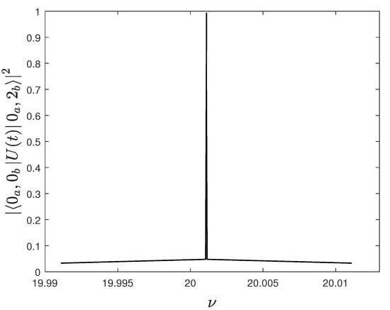
Figure 1. Time averaged transition probability $|⟨0_a,0_b\left|U\left(t\right)\right|0_a,2_b{⟩|}^2$ as a function of the modulation frequency $\nu$ generated by the time-dependent Hamiltonian (40); $\nu \approx 2{\omega }_b$, ${\omega }_b=10$, ${\omega }_a={\omega }_b/2$, $g=0.1$, and $ϵ=0.9$.

In Figure 2, we compare the exact evolution of the average photon number in the b-mode, starting with the initial vacuum state $|0_a,0_b⟩$ with the results of analytical calculations using the effective Hamiltonian (43),

$${⟨b^{†}b⟩}_{app}\approx {sinh}^2\left(2g_{eff}t\right).$$

(45)

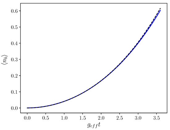
Figure 2. Evolution of the average photon number in mode b for the initial vacuum state in both modes in case of effective two-photon transition, $\nu \approx 2{\omega }_b$, where ${\omega }_b=10$, ${\omega }_a={\omega }_b/2$, $g=0.1$, and $ϵ=0.9$. The solid (blue) line corresponds to the analytic approximation (45), the dashed (black) line results from numerical calculation with the Hamiltonian (40).

3.1.1. Dicke Model with Modulated Frequency

The dynamics of the quantum Dicke model, describing the interaction between an effective S-spin system and a single mode of a quantized field with harmonically modulated atomic frequency [16,17,20,22,42] is governed by the following Hamiltonian,

$$H={\omega }_0\left[1+\gamma cos\left(\nu t\right)\right]S_z+{\omega }_1{a}^{†}a+g\left(a^{†}+a\right)\left(S_{+}+S_{-}\right),$$

(46)

where $g\ll {\omega }_{0,1}$ and, $0<ϵ={\omega }_0\gamma /\nu <1$, which corresponds to (37) with $X_{\pm }=S_{\pm }$, $X_0=S_z$ and $Y_{+}=a^{†},Y_{-}=a$, $Y_0=a^{†}a$. In this case the intensity-dependent shift (A28)–(A31) takes the form:

$$K(S_z,a^{†}a)=g{\epsilon }^{\left(1\right)}\left(ϵ\right)\left(S_z^2+\left(1+2a^{†}a\right)S_z\right)+{\epsilon }^{\left(3\right)}\left(ϵ\right){\left(a^{†}a\right)}^2{S}_z+O\left({\epsilon }^{\left(3\right)}\right),$$

where ${\epsilon }^{\left(k\right)}\sim {\epsilon }^k$, $\epsilon \sim g/l.c.(\omega ,\nu )\ll 1$, are some homogeneous polynomials on the Bessel functions $J_k\left(ϵ\right)$, $0<ϵ={\omega }_0\gamma /\nu \lesssim 1$ (A32). In particular, (i) the dynamic Stark shift term $\sim {\epsilon }_k^{\left(1\right)}\left(ϵ\right)a^{†}a{S}_z$ suppresses all transitions between the field and the atomic system with an exchange of more than one excitation; (ii) the atomic Kerr term $\sim {\epsilon }_k^{\left(1\right)}\left(ϵ\right)S_z^2$ does not allow to efficiently absorb more than one excitation by the atomic system; and (iii) the field Kerr term $\sim {\epsilon }_k^{\left(3\right)}\left(ϵ\right){\left(a^{†}a\right)}^2$ makes the generation of more than four photons by the quantum field inefficient. Thus, the resonance expansion containing only efficient transitions takes the form:

$$\begin{array}{ccc}\hfill H_{RE}^F& \approx & {\omega }_0{S}_z+{\omega }_1{a}^{†}a+\nu E_0+K(S_z,a^{†}a)+g{J}_0\left(ϵ\right)\left(a{S}_{+}+h.c.\right)\hfill \\ & & +g\sum _{k=1}{J}_k\left(ϵ\right)\left[\left(E^{†k}+{(-1)}^k{E}^k\right)a{S}_{+}+E^k{a}^{†}{S}_{+}+h.c.\right]\hfill \\ & & +g\sum _{k=1}{\epsilon }_{1k}^{\left(1\right)}\left(ϵ\right)\left(E^k{S}_{+}^2+h.c.\right)\hfill \\ & & +g\sum _{k=1}{\epsilon }_{2k}^{\left(1\right)}\left(ϵ\right)\left(E^k{a}^{†2}{S}_z+h.c.\right)+g\sum _{k=1}{\epsilon }_{3k}^{\left(3\right)}\left(ϵ\right)\left(a^{†4}{S}_z+h.c.\right).\hfill \end{array}$$

(47)

3.1.2. Non-Symmetric Excitation of an Atomic System in a Vacuum Field

The resonant expansion (47) reveals the existence of effective processes consisting in the excitation of two atoms in the symmetric configuration, described by:

$$g{\epsilon }_{1k}^{\left(1\right)}\left(ϵ\right)\left(E^k{S}_{+}^2+h.c.\right).$$

However, this process is rapidly suppressed by the atomic Kerr term $\sim S_z^2$, which is of the first order on the small parameters. Thus, the symmetry of the atomic system should be broken in order to render the two-atom excitation process efficient.

Let us consider the following generalization of the Hamiltonian (46) to the two-atom case,

$$\begin{array}{ccc}\hfill H\left(t\right)& =& \sum _{i=1}^2\left({\omega }_i+g_{0}cos\left(\nu t\right)\right)s_{zi}+{\omega }_c{a}^{†}a\hfill \\ & & +2\left(a^{†}+a\right)\sum _{i=1}^2{g}_i{s}_{xi},\hfill \end{array}$$

(48)

of which the corresponding Floquet form is:

$$\begin{array}{ccc}\hfill H^F& =& \sum _{i=1}^2{\omega }_i{s}_{zi}+{\omega }_c{a}^{†}a+\nu E_0\hfill \\ & & +g_0\left(E+E^{†}\right)\sum _{i=1}^2{s}_{zi}+2\left(a^{†}+a\right)\sum _{i=1}^2{g}_i{s}_{xi}.\hfill \end{array}$$

(49)

For simplicity, we also assume that $ϵ=g_0/\nu \ll 1$. In this case we obtain a resonant expansion, which up to the second order on the small parameters is given in Appendix B.1, Equation (A33). Instead, the Kerr term Equation (A33) contains the spin exchange operator $s_{-1}{s}_{+2}+h.c.$, which can be taken out of resonance under appropriate frequency conditions. For instance, choosing:

$$\begin{array}{ccc}\hfill {\omega }_c& =& {\omega }_1+{\omega }_2\approx \nu ,\hfill \\ \hfill g_i& \ll & |{\omega }_1-{\omega }_2|,\hfill \end{array}$$

Imposing appropriate conditions on the frequencies all of the first order transitions in (A33) can be removed thus arriving at the following effective Hamiltonian for the initial vacuum field mode:

$$H_{eff}^F\approx {\tilde{\omega }}_1{s}_{z1}+{\tilde{\omega }}_2{s}_{z2}+\nu E_0+g_{eff}\left(E{s}_{+1}{s}_{+2}+h.c.\right),$$

(50)

where $\widetilde{{\omega }_i}={\omega }_i+g_i\left({\epsilon }_{1i}+{\delta }_{1i}\right)+\mathcal{O}\left({\epsilon }^{\left(3\right)}\right)$, $ϵ=g_0/\nu$, ${\epsilon }_{1i}=g_i/({\omega }_c+{\omega }_i)$, ${\delta }_{1i}=g_i/({\omega }_i-{\omega }_c)$, and ${\epsilon }_{2i}=g_i/{\omega }_c$. The effective interaction constant is:

$$g_{eff}=ϵ\left(g_1{\epsilon }_{12}+g_2{\epsilon }_{11}-g_1{\delta }_{12}-g_2{\delta }_{11}\right).$$

The Hamiltonian (50) describes an effective excitation of two different atoms mediated by a vacuum field in the modulated Dicke model [43].

In Figure 3, we plot the time-averaged probability of two-atom excitation $|⟨0_1,0_2\left|U\left(t\right)\right|1_1,1_2{⟩|}^2$ from the vacuum as a function of the modulation frequency $\nu$, at ${\omega }_2=3{\omega }_1$ with ${\omega }_1=10$, $g_0=g_1=g_2=g=1$. The evolution operator $U\left(t\right)$ is generated by the exact Hamiltonian (48). The position of the resonance is well described by our approximation, giving $\nu ={\tilde{\omega }}_1+{\tilde{\omega }}_2\approx 4{\omega }_1-104g/\left(105{\omega }_1\right)=39.90095$.

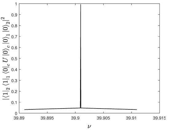
Figure 3. Time averaged transition probability $|⟨0_1,0_2\left|U\left(t\right)\right|1_1,1_2{⟩|}^2$ as a function of the modulation frequency $\nu$ generated by the time-dependent Hamiltonian (48); $\nu \approx {\omega }_1+{\omega }_2$, ${\omega }_1=10$, ${\omega }_2=3{\omega }_1$, and ${\omega }_c={\omega }_1+{\omega }_2$ with $g_0=g_1=g_2=1$.

In Figure 4 we compare the evolution of averages $⟨s_{-1}{s}_{+1}⟩$ and $⟨s_{-1}{s}_{-2}{s}_{+2}{s}_{+1}⟩$, describing the excitation of the first atom and the joint excitation of both atoms [28], and the corresponding approximate evolutions, generated by the effective Hamiltonian (50), for the initial non-excited atoms and the cavity mode in vacuum $|0_1,0_2⟩$. The approximate expressions, immediately following from (50),

$${⟨s_{-1}{s}_{+1}⟩}_{app}={⟨s_{-1}{s}_{-2}{s}_{+2}{s}_{+1}⟩}_{app}\approx {cos}^2\left(g_{eff}t\right),$$

(51)

describe the dynamics of the observables fairly well for $\nu ={\tilde{\omega }}_1+{\tilde{\omega }}_2$, ${\omega }_2=3{\omega }_1$, ${\omega }_c={\omega }_1+{\omega }_2$ with ${\omega }_1=10$, and $g_0=g_1=g_2=g=1$.

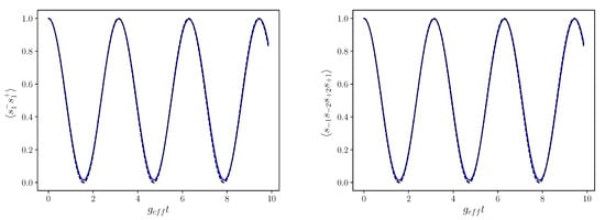
Figure 4. Evolution of the averages $⟨s_{-1}{s}_{+1}⟩$ (above) and $⟨s_{-1}{s}_{-2}{s}_{+2}{s}_{+1}⟩$ (below) for the initial non-excited atoms and the cavity mode in vacuum $|0_1,0_2⟩$; $\nu ={\tilde{\omega }}_1+{\tilde{\omega }}_2$, ${\omega }_2=3{\omega }_1$, ${\omega }_c={\omega }_1+{\omega }_2$ with ${\omega }_1=10$, and $g_0=g_1=g_2=1$; the continuous (blue) line corresponds to the numerical calculation for the exact Hamiltonian (48), the dashed (black) line corresponds to the approximation (51).

4. Conclusions

Even the simplest periodically modulated quantum systems exhibit a rich resonance structure captured by the expansion (9). This resonance expansion is obtained by a specific Lie-type perturbation theory where the coupling constant is small with respect to the bare system’s frequencies both for weak and strong modulation amplitude. In the framework of this approach the order of each resonance, which determines the width of the related transition, and consequently the Rabi frequency of corresponding oscillations can be found. In the case of single modulated linear systems, we have been able to obtain the principal contribution to the effective interaction constant corresponding to each resonant term.

Effective Hamiltonians, describing all possible resonant transitions, can be extracted from the resonance expansion by establishing some particular frequency conditions. It was observed that in the case of a single modulated system the order of effective Hamiltonians in the vicinity of each resonance is exactly the same as that of the corresponding terms in the resonance expansion.

The common feature of modulated linear (on Lie algebra generators, in our case $SU\left(2\right)$ and $SU(1,1)$) Hamiltonians is the absence of the dynamic Stark shift and Kerr-like terms in the resonance expansion. Thus, all of the resonances appearing in this expansion are efficient i.e., there are always frequency conditions such that the transition probabilities between energy levels, described by the corresponding effective Hamiltonian, are close to unity. In contrast, the effective Hamiltonians of periodically perturbed non-linear quantum systems (effective as in Section 2.5) and coupled (as in Section 4), always contain non-linearities that “select” the efficient transitions among all those present in the formal resonance expansion. The present approach can be immediately generalized to quantum systems with higher unitary symmetries, in particular, to multilevel atoms described by generators of $SU\left(N\right)$ algebra.

Appendix A.1. Frequency Corrections

Here we detail the procedure that can be applied for obtaining the higher order frequency corrections in the vicinity of the k-th resonance, $\omega \approx k\nu$.

After some algebra we find the operational coefficients $A_{\pm }$ and $B_{\pm }$ appearing in (18),

$$\begin{array}{ccc}\hfill A_{\pm }\left(\alpha ,{\alpha }^{†},\beta ,{\beta }^{†}\right)& =& A_{\pm 1}+A_{\pm 2}\frac{C\left({\eta }_{\pm }\right)-1}{{\eta }_{\pm }^2}+A_{\pm 3}\frac{S\left({\eta }_{\pm }\right)}{{\eta }_{\pm }}+A_{\pm 4}\frac{S\left({\eta }_{\pm }\right)-{\eta }_{\pm }}{{\eta }_{\pm }^3},\hfill \end{array}$$

(A11)

$$\begin{array}{ccc}\hfill B_{\pm }\left(\alpha ,{\alpha }^{†},\beta ,{\beta }^{†}\right)& =& B_{\pm 1}+B_{\pm 2}\frac{C\left({\eta }_{\pm }\right)-1}{{\eta }_{\pm }^2}+B_{\pm 3}\frac{S\left({\eta }_{\pm }\right)}{{\eta }_{\pm }}+B_{\pm 4}\frac{S\left({\eta }_{\pm }\right)-{\eta }_{\pm }}{{\eta }_{\pm }^3},\hfill \end{array}$$

(A12)

where

$$\begin{array}{ccc}\hfill A_{\pm 1}& =& \omega -\left({\tilde{\alpha }}^{†}+\tilde{\alpha }\right)\nu +g_0\left(E^{†}+E\right),\hfill \\ \hfill A_{\pm 2}& =& 4{\beta }^{†}\beta \left[\omega +g_0\left(E^{†}+E\right)\right]-2\nu \left(\tilde{\beta }{\beta }^{†}+{\tilde{\beta }}^{†}\beta \right)\hfill \\ & & -2g_1\left(E^{†}+E\right)\left({\alpha }^{†}-\alpha \right)\left({\beta }^{†}-\beta \right),\hfill \\ \hfill A_{\pm 3}& =& \pm 2g_1\left(E^{†}+E\right)\left({\beta }^{†}+\beta \right),\hfill \\ \hfill A_{\pm 4}& =& -2\nu \xi ,\hfill \end{array}$$

and

$$\begin{array}{ccc}\hfill B_{\pm 1}& =& g_1\left(E^{†}+E\right)+\nu \beta \frac{\tilde{\beta }{\beta }^{†}-{\tilde{\beta }}^{†}\beta }{2\beta {\beta }^{†}},\hfill \\ \hfill B_{\pm 2}& =& \pm \beta \left[\omega +g_0\left(E^{†}+E\right)\right]\left({\alpha }^{†}-\alpha \right)\mp \nu \left[\tilde{\beta }\left({\alpha }^{†}-\alpha \right)+\beta \left({\tilde{\alpha }}^{†}+\tilde{\alpha }\right)\right]\hfill \\ & & +g_1\left(E^{†}+E\right)\left[2\beta \left({\beta }^{†}+\beta \right)+{\left({\alpha }^{†}-\alpha \right)}^2\right],\hfill \\ \hfill B_{\pm 3}& =& -\beta \left[\omega +g_0\left(E^{†}+E\right)\right]+g_1\beta \left(E^{†}+E\right)\left({\alpha }^{†}-\alpha \right)+\nu \beta \frac{\tilde{\beta }{\beta }^{†}+{\tilde{\beta }}^{†}\beta }{2\beta {\beta }^{†}},\hfill \\ \hfill B_{\pm 4}& =& \mp \nu \beta \frac{\xi \left({\alpha }^{†}-\alpha \right)}{2\beta {\beta }^{†}},\hfill \end{array}$$

here $C\left({\eta }_{\pm }\right)=cos{\eta }_{\pm },cosh{\eta }_{\pm }$, $S\left({\eta }_{\pm }\right)=sin{\eta }_{\pm },sinh{\eta }_{\pm }$, correspond to $SU\left(2\right)$ and $SU(1,1)$ algebras respectively, with:

$$\begin{array}{ccc}\hfill {\eta }_{\pm }& =& \sqrt{4{\beta }^{†}\beta \mp {\left({\alpha }^{†}-\alpha \right)}^2},\hfill \\ \hfill \xi & =& 2{\beta }^{†}\beta \left({\tilde{\alpha }}^{†}+\tilde{\alpha }\right)+\left({\alpha }^{†}-\alpha \right)\left(\tilde{\beta }{\beta }^{†}-{\tilde{\beta }}^{†}\beta \right).\hfill \end{array}$$

The operators $\tilde{\alpha }$ and $\tilde{\beta }$ admit the following expansion on the small parameter $\epsilon$,

$$\tilde{\alpha }=\sum _{j=1}j{a}_j{E}^j,\tilde{\beta }=\sum _{j=1}j\left(b_j{E}^j-c_j{E}^{†j}\right),$$

where

$$x_{\pm j}=\sum _m{x}_{\pm j}^{\left(m\right)},x_{\pm j}^{\left(m\right)}\sim {\epsilon }^{(j+2m)},x_{\pm j}=a_{\pm j},b_{\pm j},c_{\pm j},$$

(A13)

except for $b_{\pm 0}=c_{\pm 0}=\sum b_{\pm 0}^{\left(m\right)}$, with $b_{\pm 0}^{\left(m\right)}\sim {\epsilon }^{(2m+2)}$.

Expanding $A_{\pm }$ and $B_{\pm }$ in series according to (A13) and equaling $O_{\pm }^{†}{H}^F{O}_{\pm }$ to $H_{\pm (k+1)}$ up to ${\epsilon }^{\left(k\right)}$ as in (13), one can determine the required coefficients $x_{\pm j}^{\left(m\right)},m\le k$ and find the corrected frequency ${\tilde{\omega }}_{\pm (k+1)}$.

Let us consider, for instance, the effective Hamiltonian (13) in the vicinity of the second-order resonance, $k=1$,

$$H_{\pm 2}^F={\tilde{\omega }}_{\pm 2}{X}_0+\nu E_0+{ϵ}_{\pm 1}\left(E^2{X}_{+}+E^{†2}{X}_{-}\right)+\mathcal{O}\left({\epsilon }^{\left(2\right)}\right).$$

In this case it is sufficient to expand the coefficients (A11) and (A12) up to the first order on the small parameters, obtaining:

$$\begin{array}{}\mathrm{(A14)}& \hfill A_{\pm }\left(\alpha ,{\alpha }^{†},\beta ,{\beta }^{†}\right)& =& \omega \mp 2\omega \left(b_1^{\left(0\right)2}+c_1^{\left(0\right)2}\right)\pm 2\nu \left(b_1^{\left(0\right)2}-c_1^{\left(0\right)2}\right)\pm 4g_1\left(b_1^{\left(0\right)}+c_1^{\left(0\right)}\right)\hfill \mathrm{(A15)}& & & +\left(g_0-\nu a_1^{\left(0\right)}\right)\left(E+E^{†}\right)\hfill \mathrm{(A16)}& & & +\left[-2\nu a_2^0\pm 2g_1\left(b_1^{\left(0\right)}+c_1^{\left(0\right)}\right)\mp 2\omega b_1^{\left(0\right)}{c}_1^{\left(0\right)}\right]\left(E^2+E^{†2}\right),\hfill \end{array}$$

and

$$\begin{array}{}\mathrm{(A17)}& \hfill B_{\pm }\left(\alpha ,{\alpha }^{†},\beta ,{\beta }^{†}\right)& =& -2\omega b_0^{\left(0\right)}+\left(\nu a_1^{\left(0\right)}-g_0\right)\left(b_1^{\left(0\right)}+c_1^{\left(0\right)}\right)-\frac{\omega }{2}{a}_1^{\left(0\right)}\left(b_1^{\left(0\right)}-c_1^{\left(0\right)}\right)\hfill \mathrm{(A18)}& & & +\left(g_1-\omega b_1^{\left(0\right)}+\nu b_1^{\left(0\right)}\right)E+\left(g_1-\omega c_1^{\left(0\right)}-\nu c_1^{\left(0\right)}\right)E^{†}\hfill \mathrm{(A19)}& & & -\left[\left(2\nu +\omega \right)c_2^{\left(0\right)}+\frac{\omega }{2}{a}_1^{\left(0\right)}{c}_1^{\left(0\right)}\right])E^{†2}\hfill \mathrm{(A20)}& & & +\left[\left(2\nu -\omega \right)b_2^{\left(0\right)}+\frac{\omega }{2}{a}_1^{\left(0\right)}{b}_1^{\left(0\right)}\right]E^2.\hfill \end{array}$$

Equaling $H_{\pm 2}^F$ to $O_{\pm }^{†}{H}^F{O}_{\pm }$ according to the general procedure (18),

$$\begin{array}{ccc}\hfill {\tilde{\omega }}_{\pm 2}{X}_0+\nu E_0+{ϵ}_{\pm 1}\left(E^2{X}_{+}+E^{†2}{X}_{-}\right)+\mathcal{O}\left({\epsilon }^{\left(2\right)}\right)& =& A_{\pm }\left({\alpha }_{\pm },{\alpha }_{\pm }^{†},{\beta }_{\pm },{\beta }_{\pm }^{†}\right)X_0+\nu E_0\hfill \\ & & +B_{\pm }\left({\alpha }_{\pm },{\alpha }_{\pm }^{†},{\beta }_{\pm },{\beta }_{\pm }^{†}\right)X_{+}+h.c.,\hfill \end{array}$$

(A21)

one can immediately observe that (i) Equation (A14) gives the frequency correction; (ii) the parameters $x_{\pm 1}$ (A13) are obtained by equaling to zero Equations (A15)–(A19), giving in particular:

$$b_1^{\left(0\right)}=\frac{g_1}{\omega -\nu }{c}_1^{\left(0\right)}=\frac{g_1}{\omega +\nu }.$$

(A22)

which are required for the first correction to the frequency $\omega$.

Substituting (A22) to (A14) we arrive at the first order correction, which is valid close to any resonance except the principal one, $\omega =k\nu$, $k>1$,

$${\tilde{\omega }}_{\pm 2}=\omega \pm \frac{4\omega g_1}{{\omega }^2-{\nu }^2}+\mathcal{O}\left({\epsilon }^{\left(3\right)}\right).$$

(A23)

The above procedure is directly generalizable to the order ${\epsilon }^{\left(k\right)}$, required for determination of the frequency corrections in the vicinity of the k-th resonance.

Appendix B.1. Non-Symmetric Excitation of an Atomic System in a Vacuum

Applying an elimination procedure similar to that described in Appendix A to the Hamiltonian (49) we arrive at the following resonance expansion up to the second order on $ϵ$:

$$\begin{array}{ccc}\hfill H_{RE}^F& \approx & \sum _{i=1}^2\left({\omega }_i+g_i{\epsilon }_{1i}\right)s_{zi}+{\omega }_c{a}^{†}a+\nu E_0\hfill \\ & & +2g_1\sum _{i=1}^2\left({\omega }_i+g_i{\epsilon }_{1i}\right)a^{†}a{s}_{zi}-g_2{\epsilon }_{11}\left(s_{-1}{s}_{+2}+h.c.\right)\hfill \\ & & +\sum _{i=1}^2{g}_i\left[\left(1+ϵ\left(E^{†}-E\right)+\frac{{ϵ}^2}{2}\left(E^{†2}+E^2\right)\right)a{s}_{+i}+h.c.\right]\hfill \\ & & -\sum _{i=1}^2{g}_i\left[\left(E-\frac{ϵ}{2}{E}^2\right)a^{†}{s}_{+i}+h.c.\right]-\sum _{i=1}^2{g}_i{\epsilon }_{1i}{\epsilon }_{2i}\left(a^3{s}_{+i}+h.c.\right)\hfill \\ & & +2\sum _{i=1}^2{g}_iϵ{\epsilon }_{1i}\left(E^{†}{a}^2+h.c.\right)s_{zi}\hfill \\ & & +ϵ\left(g_1{\epsilon }_{12}-g_2{\epsilon }_{11}\right)\left(E^{†}{s}_{-1}{s}_{+2}-E{s}_{-1}{s}_{+2}+h.c.\right)\hfill \\ & & +ϵ\left(g_1{\epsilon }_{12}+g_2{\epsilon }_{11}\right)\left(E{s}_{+1}{s}_{+2}+h.c.\right),\hfill \end{array}$$

(A33)

where $ϵ=g_0/\nu$, ${\epsilon }_{1i}=g_i/({\omega }_c+{\omega }_i)$, and ${\epsilon }_{2i}=g_i/{\omega }_c$.

References

- Autler, S.H.; Townes, C.H. Stark Effect in Rapidly Varying Fields. Phys. Rev. 1995, 100, 703–722. [Google Scholar] [CrossRef]
- Shirley, J.H. Solution of the Schrödinger Equation with a Hamiltonian Periodic in Time. Phys. Rev. 1965, 138, B979–B987. [Google Scholar] [CrossRef]
- Margerie, J.; Brossel, J. Transitions à plusieurs quanta électromagnétiques. Acad. Sci. 1955, 241, 373. [Google Scholar]
- Yabuzaki, T.; Nakayama, S.; Murakami, Y.; Ogawa, T. Interaction between a spin-1/2 atom and a strong rf field. Phys. Rev. A 1974, 10, 241–243. [Google Scholar] [CrossRef]
- Grossmann, F.; Dittrich, T.; Jung, P.; Hänggi, P. Coherent destruction of tunneling. Phys. Rev. Lett. 1991, 67, 516–519. [Google Scholar] [CrossRef] [PubMed]
- Dakhnovskii, Y.; Metiu, H. Conditions leading to intense low-frequency generation and strong localization in two-level systems. Phys. Rev. A 1993, 48, 2342–2345. [Google Scholar] [CrossRef]
- Zhao, X.G. Quasienergy and Floquet states in a time-periodic driven two-level system. Phys. Rev. B 1994, 49, 16753–16756. [Google Scholar] [CrossRef] [PubMed]
- Wang, H.; Freire, V.N.; Zhao, X.G. Emission spectrum in driven two-level systems. Phys. Rev. A 1998, 58, 1531–1536. [Google Scholar] [CrossRef]
- Seideman, T.J. New means of spatially manipulating molecules with light. Chem. Phys. 1999, 111, 4397–43405. [Google Scholar] [CrossRef]
- Larsen, J.J.; Hald, K.; Bjerre, N.; Stapelfeld, H.; Seideman, T.J. Three dimensional alignment of molecules using elliptically polarized laser fields. Phys. Rev. Lett. 2000, 85, 2470–2473. [Google Scholar] [CrossRef]
- Dey, B.K.; Shapiro, M.; Brumer, P. Coherently controlled nanoscale molecular deposition. Phys. Rev. Lett. 2000, 85, 3125–3128. [Google Scholar] [CrossRef] [PubMed]
- Stapelfeld, H.; Seideman, T. Colloquium: Aligning molecules with strong laser pulses. Rev. Mod. Phys. 2003, 75, 543–557. [Google Scholar] [CrossRef]
- Martinez, D.F. Floquet–Green function formalism for harmonically driven Hamiltonians. J. Phys. A Math. Gen. 2003, 36, 9827–9842. [Google Scholar] [CrossRef]
- Creffield, C.E. Location of crossings in the Floquet spectrum of a driven two-level system. Phys. Rev. B 2003, 67, 165301. [Google Scholar] [CrossRef]
- Yan, Y.; Lü, Z.; Zheng, H. Bloch-Siegert shift of the Rabi model. Phys. Rev. A 2015, 91, 053834. [Google Scholar] [CrossRef]
- Huang, J.F.; Liao, J.Q.; Tian, L.; Kuang, L.M. Manipulating counter-rotating interactions in the quantum Rabi model via modulation of transition frequency of the two-level system. Phys. Rev. A 2017, 96, 043849. [Google Scholar] [CrossRef]
- Zhao, Y.J.; Liu, Y.L.; Liu, Y.X.; Nori, F. Generating nonclassical photon states via longitudinal couplings between superconducting qubits and microwave fields. Phys. Rev. A 2015, 91, 053820. [Google Scholar] [CrossRef]
- Casanova, J.; Puebla, R.; Moya-Cessa, H.; Plenio, M.B. Connecting nth order generalised quantum Rabi models: Emergence of nonlinear spin-boson coupling via spin rotations. NPJ Quantum Inf. 2018, 4, 1–7. [Google Scholar] [CrossRef]
- Pietikäinen, I.; Danilin, S.; Kumar, K.S.; Vepsäläinen, A.; Golubev, D.S.; Tuorila, J.; Paraoanu, G.S. Observation of the Bloch-Siegert shift in a driven quantum-to-classical transition. Phys. Rev. B 2017, 96, 020501(R). [Google Scholar] [CrossRef]
- Navarrete-Benllochi, C.; García-Ripoll, J.J.; Porras, D. Inducing Nonclassical Lasing via Periodic Drivings in Circuit Quantum Electrodynamics. Phys. Rev. Lett. 2014, 113, 193601. [Google Scholar] [CrossRef] [PubMed]
- Wang, G.; Xiao, R.; Shen, H.Z.; Sun, C.; Xue, K. Simulating Anisotropic quantum Rabi model via frequency modulation. Sci. Rep. 2019, 9, 1–10. [Google Scholar] [CrossRef] [PubMed]
- Hoeb, F.; Angaroni, F.; Zoller, J.; Calarco, T.; Strini, G.; Montangero, S.; Benenti, G. Amplification of the parametric dynamical Casimir effect via optimal control. Phys.Rev. A 2017, 96, 033851. [Google Scholar] [CrossRef]
- Dodonov, A.V. Dynamical Casimir effect via four- and five-photon transitions using a strongly detuned atom. Phys. Rev. A 2019, 100, 032510. [Google Scholar] [CrossRef]
- Louisell, W.H.; Yariv, A.; Siegman, A.E. Quantum Fluctuations and Noise in Parametric Processes. I. Phys. Rev. 1961, 124, 1646–1654. [Google Scholar] [CrossRef]
- Klimov, A.B.; Sainz, I.; Chumakov, S.M. Resonance expansion versus the rotating-wave approximation. Phys. Rev. A 2003, 68, 063811. [Google Scholar] [CrossRef]
- Ma, K.K.W.; Law, C.K. Three-photon resonance and adiabatic passage in the large-detuning Rabi model. Phys. Rev. A 2015, 92, 023842. [Google Scholar] [CrossRef]
- Sokolov, A.M.; Stolyarov, E.V. Single-photon switch controlled by a qubit embedded in an engineered electromagnetic environment. Phys. Rev. A 2020, 102, 042306. [Google Scholar] [CrossRef]
- Garziano, L.; Macrì, V.; Stassi, R. One Photon Can Simultaneously Excite Two or More Atoms. Phys. Rev. Lett. 2016, 117, 043601. [Google Scholar] [CrossRef] [PubMed]
- Niemczyk, T.; Deppe, F.; Huebl, H.; Menzel, E.P.; Hocke, F.; Schwarz, M.J.; Garcia-Ripoll, J.J.; Zueco, D.; Hümmer, T.; Solano, E.; et al. Circuit quantum electrodynamics in the ultrastrong-coupling regime. Nature Phys. 2010, 6, 772–776. [Google Scholar] [CrossRef]
- Schoelkopf, R.J.; Girvin, S.M. Wiring up quantum systems. Nature 2008, 451, 664–669. [Google Scholar] [CrossRef] [PubMed]
- You, J.; Nori, F. Atomic physics and quantum optics using superconducting circuits. Nature 2011, 474, 589–597. [Google Scholar] [CrossRef]
- Blais, A.; Grimsmo, A.L.; Girvin, S.M.; Wallraff, A. Circuit Quantum Electrodynamics. arXiv 2020, arXiv:2005.12667v1. [Google Scholar]
- Klimov, A.B.; Sánchez-Soto, L.L. Method of small rotations and effective Hamiltonians in nonlinear quantum optics. Phys. Rev. A 2000, 61, 068302. [Google Scholar] [CrossRef]
- Klimov, A.B.; Sánchez-Soto, L.L.; Navarro, A.; Yustas, E.C. Effective Hamiltonians in quantum optics: A systematic approach. J. Mod. Opt. 2002, 49, 2211–2226. [Google Scholar] [CrossRef]
- Sainz, I.; Klimov, A.B.; Saavedra, C. Effective Hamiltonian approach to periodically perturbed quantum optical systems. Phys. Lett. A 2006, 351, 26–30. [Google Scholar] [CrossRef]
- Comtet, L. Advanced Combinatorics; Riedel, D., Ed.; Publishing Co.: Dordrecht, The Netherlands, 1974. [Google Scholar]
- Karassiov, V.P. G-invariant polynomial extensions of Lie algebras in quantum many-body physics. J. Phys. A Math. Gen. 1994, 27, 153. [Google Scholar] [CrossRef]
- Karassiov, V.P.; Klimov, A.B. An algebraic approach for solving evolution problems in some nonlinear quantum models. Phys. Lett. A 1994, 191, 117. [Google Scholar] [CrossRef]
- Lee, Y.-H.; Yang, W.-L.; Zhang, Y.-Z. Polynomial algebras and exact solutions of general quantum nonlinear optical models I: Two-mode boson systems. J. Phys. A Math. Theor. 2010, 43, 185204. [Google Scholar] [CrossRef]
- Graefe, E.-M.; Korsch, H.J.; Rush, A. Classical-quantum correspondence in bosonic two-mode conversion systems: Polynomial algebras and Kummer shapes. Phys. Rev. A 2016, 93, 042102. [Google Scholar] [CrossRef]
- Roy, A.; Devoret, M. Introduction to Quantum-limited Parametric Amplification of Quantum Signals with Josephson Circuits. Comptes Rendus Phys. 2016, 17, 740–755. [Google Scholar] [CrossRef]
- Chen, Z.; Wang, Y.; Li, T.; Qiu, Y.; Inomata, K.; Yoshihara, F.; Han, S.; Nori, F.; Tsai, J.S.; You, J.Q. Single-photon-driven high-order sideband transitions in an ultrastrongly coupled circuit-quantum-electrodynamics system. Phys. Rev. A 2017, 96, 012325. [Google Scholar] [CrossRef]
- Dodonov, A.V.; Dodonov, V.V. Dynamical Casimir effect in two-atom cavity QED. Phys. Rev. A 2012, 85, 055805. [Google Scholar] [CrossRef]
Publisher’s Note: MDPI stays neutral with regard to jurisdictional claims in published maps and institutional affiliations. |
© 2021 by the authors. Licensee MDPI, Basel, Switzerland. This article is an open access article distributed under the terms and conditions of the Creative Commons Attribution (CC BY) license (http://creativecommons.org/licenses/by/4.0/).