Investigation on the Manufacturing, Testing, and Simulation Processes of the Hood Hinge Assembly

Abstract

The automotive industry is currently undergoing significant transformations driven by challenges such as fierce competition, supply chain disruptions, and stringent legislative regulations aimed at reducing pollutant emissions. The research employs a combination of theoretical analysis and numerical modeling to investigate the manufacturing processes of stamped automotive components. Data collection methods include experimental testing of materials, LS-DYNA simulations, and non-contact scanning for dimensional analysis. The study also utilizes a workflow diagram to illustrate the various phases involved in the design and validation of automotive assemblies. The findings detail the critical role of digital transformation in the automotive industry, particularly in enhancing the accuracy and reliability of manufacturing processes. Implementing digital twins improves product quality and reduces product development time. The experimental results were compared with simulation data, and a good correlation was identified, showing, for the numerical model with complete history (thickness and stress), a difference of $1.6\%$. Furthermore, to simplify the process of developing the numerical models for the initial iterations, a scale factor of $~1.1$ is proposed for the testing load. This factor is not limited to the current design, as the manufacturing stages are similar for this range of products.

1. Introduction

The automotive industry, over the past 20 years, has probably been going through its most dynamic period of transformation and adaptation. Every day, new market challenges from stakeholders [1], energy efficiency [2], new requirements, advanced manufacturing solutions [3], and legislative regulations emerge. Car manufacturers have to implement these updates during development or, sometimes, on the fly, even after the start of series production. Currently, referring to the car manufacturing industry [1] there are new technologies and terms that making their presence: Industry 4.0 and use of machine learning instruments [2], advance to Industry 5.0 [3], development of high end robots [4], interconnecting machines by Internet of Things [5], 3D printing for prototypes and some industrial application [6], emerging industrial processes [7], automated production [8], lean manufacturing, electrification, and autonomous vehicles [9]. For European manufacturers, new challenges arise every day, dictated by market requirements, the legislation in force, and global competition.

The concept of “Industry 4.0” was first introduced in an article published by the German Government in 2011 to define a high-tech strategy for 2020. Industry 4.0 is a complex technological system that has been widely discussed and researched, with a significant influence on the industrial sector, and which introduces new concepts and technologies in industrial development: Internet of Things (IoT), Internet of Services (IoS), Augmented Reality (AR), robotics, virtual manufacturing (Cloud Manufacturing) [10,11].

One of the biggest challenges in the automotive industry is reducing pollutants and greenhouse gas emissions. Currently, the legislative norms in force impose increasingly stringent carbon-emission limits, leading manufacturers to seek a balance between a vehicle’s mass and its dynamic performance and fuel consumption by updating powertrains’ performances while simultaneously reducing the vehicle’s own mass [12,13].

This is how the concept of digitalization or digital transformation emerged [3] in terms of products and their related processes. The Digital Twin was first defined in aeronautics in 2010 as an integrated, probabilistic, multi-physics, multi-scale simulation of a vehicle or system that uses the best physical models, up-to-date sensors, and fleet history to provide a virtual mirror of the real twin’s life. The digital twin is ultra-realistic and can model one or more critical, interdependent systems of the vehicle, including propulsion, energy storage, safety devices, vehicle structure, thermal management, etc. [10,14]. The benefits of using a digital twin are numerous, including higher quality, rapid integration into master planning, reduced development time, reduced project complexity, and the adaptation of manufacturing processes to new models with minimal changes to production systems.

All these challenges affect the less visible domain for the end customer: suppliers of components, manufacturing equipment, or various services. A significant impact is on the level of suppliers developing parts and components: the time allocated to the product development and validation stages has decreased, new security and regulatory requirements have been imposed, and together with a significant trend of reducing all costs [5].

Finite element simulation [15,16,17] of mechanical processes play a crucial role in engineering. From an economic point of view, finite element simulation brings a considerable reduction in associated expenses through optimal component design [18]. Numerical models are an effective tool for performance evaluation, structure monitoring, and damage detection [19], lifetime estimation [20,21] and identification of optimal maintenance methods [22].

Numerical tools are helpful for better understanding the physical mechanisms that control the strength, ductility, and failure mode of threaded assemblies. The current progress in numerical modeling tools and methods requires that numerical models meet the accuracy and reliability requirements for their results. The use of simple design and evaluation procedures cannot fully capture the behavior of many structures unless they are updated and calibrated using large models.

The success of these numerical predictions depends on the quality of the constitutive model adopted, including the identification of the material parameters [20]. The manufacturing process analysis plays a significant role as it provides the input data for structural analyses. In this paper, a complex procedure is presented that shows, step by step, the prerequisites for accurate numerical simulations. To allow rapid analyses, the use of scale factors is discussed, and a solution is proposed for components of the hood-hinges family.

2. Materials

2.1. Hood Hinge Assembly

Developing a mechanism to open a vehicle hood is a complex task that requires specific engineering skills. Previous practical experience, cost orientation, weight reduction, and performance are some key elements considered in the design activities. Hood hinges are usually simple mechanisms made up of three main elements: a fixed element, in contact with the vehicle body, a movable element in contact with the hood, and a rotation axis to ensure the rotation of the hood during maneuvering [23]. First, their role is to facilitate access to the engine compartment (for periodic maintenance performed by the user or for more complex work carried out in service units). Additional constraints are defined by the assembly process, which requires precise tolerances and significant effort. Regarding the vehicle, passive safety measures require that, in the event of an impact, the consequences be minimal. The most common road accidents are those in which the vehicle collides with the front end [24,25]. Therefore, the need for special constructions with multiple functions is identified [26,27,28].

Thus, it is necessary to maintain the hood in the closed position when considering the vehicle’s passengers and to define a deformation space when vulnerable road users (pedestrians, cyclists, or moped users) are involved.

The car manufacturer documents the mechanical system’s operating requirements and further analyzes and validates them with the supplier. Figure 1 presents the component elements of the hood hinge assembly.

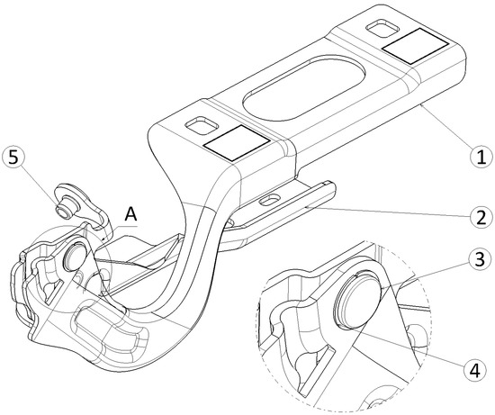
Figure 1. Hood hinge assembly: (1)—mobile part; (2)—fixed part; (3)—shaft; (4)—friction seal (detail A); (5)—link (detail A).

The initial model includes the necessary functional elements. The level of detail of the initial model depends on the information available to the supplier during the technical solution development phase.

The complex tasks that will be performed simultaneously during the design process and product validation are related (and not limited) to the following stages: (Figure 2):

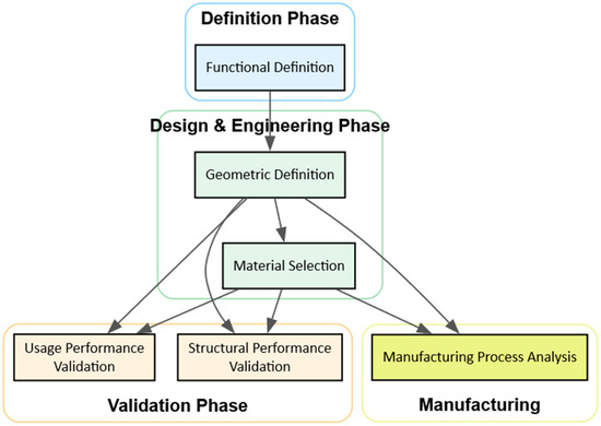
Figure 2. Workflow. The diagram presents the workflow and the connections between operations.

−

functional definition of the assembly;

−

geometric definition of the assembly;

−

manufacturing process analysis;

−

material selection;

−

usage performance validation;

−

structural performance validation.

Figure 2 shows that the process is not linear and that design loops are necessary to develop a functional and reliable product.

The functional definitions of the assembly are related to the following requirements:

−

to guarantee the hood functionality in opening/closing durability;

−

ensure a maximum angle of hood opening;

−

no radial and axial gap;

−

lateral stiffness;

−

hood maintained on hinges stop;

−

resist the exceptional forces: Strong wind on the hood maintained on the hinges stop;

−

resist the exceptional forces: High speed frontal crash;

−

repairability crash;

−

temperature in the current rolling conditions;

−

thermal and climatic behavior;

−

guarantee the maintenance of the security position;

−

maintaining the hinge during the mounting.

Given the limited information, a basic model (Figure 3a) is selected for design optimization. Technical validation is the supplier’s responsibility, so intervention was necessary to reinforce the part’s structure.

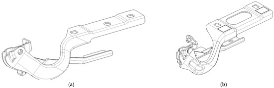
Figure 3. Design of the assembly: (a) preliminary design; (b) final design.

The final shape of the assembly indicates the addition of reinforcement elements and dome cutouts to optimize the part’s mass (Figure 3b).

To match current design trends and safety requirements, the mobile part of the assembly features a critical feature: a goose-neck-like shape between the connecting plate and the rotation axis. This design feature is not structurally favorable; thus, it requires multiple actions to define a functional part. To stiffen the structure, it is designed as a C-shaped section. Although intended to increase structural capacity, these added design features should be implemented with care, as they can affect thickness during manufacturing. The loads are bending dominant, and thickness determines the formation of plastic hinges, leading to structural failure [29]. At the same time, material selection is a critical step in the design process. The material is also challenging for the manufacturing process, as it determines the forming capability.

2.2. Material Modeling

The material was selected based on previous experience and following simple numerical simulations. The required mechanical response was achieved using S460 structural steel [30,31].

From the actual blanks used in the manufacturing process, a series of samples was extracted. As the blank’s rolling direction is unknown, the specimens were extracted according to the configuration shown in Figure 4a. Figure 4b presents the set of samples prepared, while Figure 4c presents the results of the tensile tests.

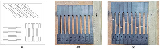
Figure 4. Samples for the tensile tests: (a) cutting solutions; (b) collection of samples; (c) tested samples (the corresponding set ID is marked on the sample).

The specimens were tested using a computer-controlled universal testing machine (Figure 5a). A mechanical extensometer was fitted to the specimens for direct measurement of elongation (Figure 5b). The testing protocol follows the mechanical characterization specification for the materials and includes three stages: pre-load, loading, and high-speed separation. The results were cumulated and compared to the reference values specific to S460 steel. As can be noticed (Figure 5c), in all cases the values of $R_{p\mathrm{0,2}}$—proportionality limits and $R_m$—maximum stress is within the prescribed range.

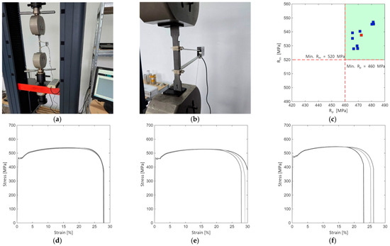
Figure 5. Testing of samples: (a) universal testing machine; (b) extensometer fitted on the sample; (c) collection of $R_{p\mathrm{0,2}}$ and $R_m$; (d) engineering stress-strain curves for set 1; (e) engineering stress-strain curves for set 2; (f) engineering stress-strain curves for set 3.

Equations set (1) are used to convert measured (engineering) stress—strain data to the true values:

$$\begin{array}{c}{\epsilon }_t=\mathrm{l}\mathrm{o}\mathrm{g}\left({1+\epsilon }_e\right)\\ {\sigma }_t={\sigma }_e·\left({1+\epsilon }_e\right)\end{array}$$

(1)

where:

−

$\left({\epsilon }_e,{\sigma }_e\right)$ define the measure dataset;

−

$\left({\epsilon }_t,{\sigma }_t\right)$ define the true stress strain dataset.

The maximum stress was identified from the curves, and the data were subsequently extracted before degradation. Figure 6 presents the resulting stress–strain curves.

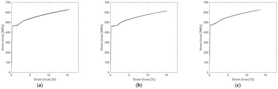
Figure 6. True stress—strain curves: (a) set 1; (b) set 2; (c) set 3.

A numerical model of the samples (Figure 7a) for calibrating the material model was developed, following the LS-Dyna nomenclature. Material *MAT_PIECEWISE_LINEAR_PLASTICITY was selected due to its versatility [32]. The material model can also be adapted to capture the degradation phase following the maximum stress [33].

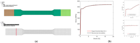
Figure 7. Model for the calibration of the material: (a) numerical model of the sample; (b) experimental vs. numerical results.

The implicit solver (*CONTROL_IMPLICIT) was used to solve the numerical model. The clamped ends were modeled as rigid bodies to impose both fixed and moving sections. To measure the force, a set of nodes located in the vicinity of the fixed end was constrained (*BOUNDARY_SPC). Two nodes on the calibrated section of the specimen, at the same distance as the extensometer opening, were selected to measure elongation during tensile loading. The simulation results (Figure 7b) were compared with the measured dataset to evaluate the performance of the implemented material model. A summary of the physical and mechanical properties of S460 is presented in Table 1.

Table 1. S460 structural steel. Physical and mechanical properties.

Parameter	Symbol	Value	Units
Density	$\rho$	$7800$	$\mathrm{kg}/{\mathrm{m}}^2$
Young modulus	$E$	$\mathrm{21,000}$	$\mathrm{M}\mathrm{P}\mathrm{a}$
Yield stress	$R_p$	min. 460	$\mathrm{M}\mathrm{P}\mathrm{a}$
Tensile strength *	$R_m$	min. 520	$\mathrm{M}\mathrm{P}\mathrm{a}$
Tensile strength +	${\sigma }_m$	min. 610	$\mathrm{M}\mathrm{P}\mathrm{a}$
Elongation	$A$	min. 20	$\%$

* The value refers to the engineering stress /⁺ The value refers to the true stress.

Cross-analysis of experimental and numerical results is an essential step in validating the material model. If differences between the two sets of results are identified, the material model requires revision, or the experimental setup was unable to provide accurate data.

3. Manufacturing Process and Simulation

3.1. Industrial Process

The manufacturing process for the assembly’s components involves a multi-step forming process. Figure 8 presents the press equipped with the dies for the forming operations. The initial shape presented in Figure 8 was previously cut from a blank sheet to match the final shape of the part.

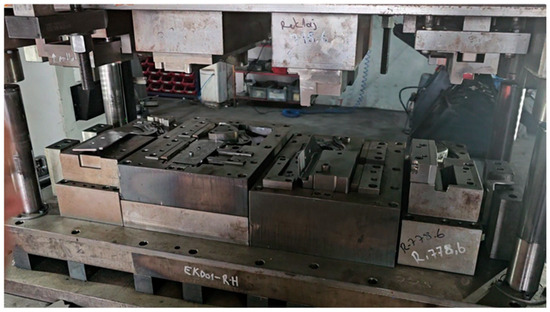
Figure 8. Press equipped with the forming dies.

Figure 9 shows the part after each forming operation. The process begins with the workpiece being extracted from the blank sheet (Figure 9a), followed by four stages of forming (Figure 9b–e). To ensure accurate positioning of the part during forming, circular cutouts are required for the guidance pins (Figure 9a–e). The final stage involves trimming to obtain the finished part (Figure 9f).

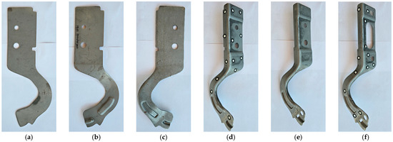
Figure 9. Forming stages: (a) workpiece; (b) stage I—construction of reinforced area and one edge of the C shape of the goose-neck section; (c) stage II—construction of second edge of the C shape; (d) stage III—90° bend; (e) stage IV—cuts in the stopper area and the axis; (f) stage V—cuts in the fixation area.

3.2. Numerical Simulation of the Forming Process

In most cases, the evaluation of the assembly’s structural performance is based on the nominal geometric definitions of the components. Thus, there are no changes in the material thickness or residual stress due to the manufacturing process that affect performance. Furthermore, performing complex analyses during design iterations is time-consuming and not justified during the design phase. A complete chain of design–manufacture–testing processes provides an opportunity to investigate the methods used during the design activity. Figure 10 gives a global perspective of simulation models developed for the forming process.

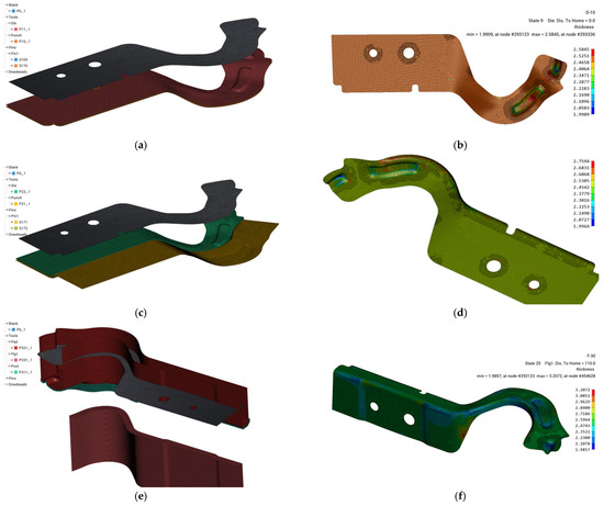
Figure 10. Forming set-ups for numerical simulation: (a) stage I tooling; (b) stage I—thickness distribution; (c) stage II tooling; (d) stage II—thickness distribution; (e) stage III tooling; (f) stage III—thickness distribution.

The numerical models for the workpiece, die, punch, and pins were constructed by extracting specific features from the geometrical model. Figure 10a presents the forming set-up for the shape presented in Figure 9b, while Figure 10b presents the thickness of the part. Figure 10c presents the forming setup for the shape shown in Figure 9c, along with the estimated thickness (Figure 10d). The final numerical setup (Figure 10e) was defined for the shape shown in Figure 9d. The resulting thickness distribution is presented in Figure 10f. The numerical simulation process was limited to stage III, as at this step, all the operations involved in forming were performed.

The numerical models were developed using ANSYS Forming 2025R1, which uses the LS-Dyna [34] as a solver. Thus, the entire simulation process is integrated into a single solver to facilitate the data exchange between various simulation stages [35,36].

The forming analysis includes, by default, mesh adaptation and refinement options. Thus, the number of elements increases substantially at the end of the simulation. The final step is a springback analysis for the stress release [37,38,39]. The solver facilitates the export of simulation results in a.dynain file in ASCII format.

3.3. Scan from the Manufactured Part

Dimensional control is performed only on the finished part; thus, during manufacturing, there are no intermediate steps to verify the part’s dimensional accuracy. Non–contact scanning methods are versatile tools for dimensional analysis and surface reconstruction. The physical shape obtained from stage III of the manufacturing process was scanned using a laser device. The geometrical model [40] was cleaned and checked for errors. To facilitate further manipulation, the STL (Stereolithography) geometry was saved in.ply (Polygon File Format) format.

Figure 11 presents the geometrical model of the scanned shape.

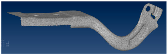
Figure 11. Scan of the manufactured part after stage III of the process.

The scanning process was performed in a floating reference system. Therefore, a method is necessary to align the scanned model with the nominal geometry. A MATLAB application was developed to manipulate geometrical data. The first step was to evaluate the surface normals. Equation set (2) provides the data required to determine the components of the normal vector starting from the cross product of two vectors defined by two edges of a triangle.

$$\begin{array}{c}\overline{n}=\left[\begin{array}{ccc}\overline{i}& \overline{j}& \overline{k}\\ u_{12}& v_{12}& w_{12}\\ u_{13}& v_{13}& w_{13}\end{array}\right]\\ u_{ij}={\displaystyle \frac{x_i-x_j}{d_{ij}}}\\ v_{ij}={\displaystyle \frac{y_i-y_j}{d_{ij}}}\\ w_{ij}={\displaystyle \frac{z_i-z_j}{d_{ij}}}\\ d_{ij}=\sqrt{{\left(x_i-x_j\right)}^2+{\left(y_i-y_j\right)}^2+{\left(z_i-z_j\right)}^2}\end{array}$$

(2)

Figure 12a presents the scanned part and the normal of the triangular entities. The algorithm operates with directional vectors computed for a specific element. Subsequently, all triangular elements were interrogated to create sets of elements with common normals (Figure 12b). The user can select a set to serve as the reference for the geometrical operations (Figure 12c).

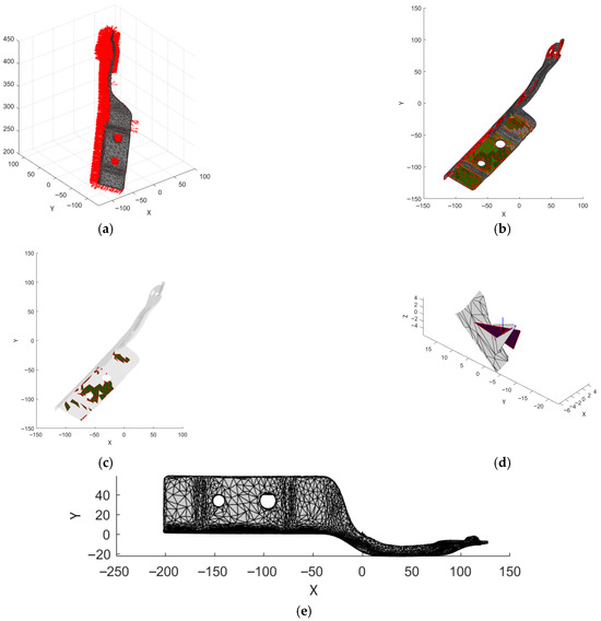
Figure 12. Geometrical operations (dimensions are represented in $\mathrm{mm}$): (a) normals; (b) definition of triangles’ sets; (c) reference set for alignment; (d) local vs. global coordinate systems; (e) aligned model.

From the selected set, the element with the largest area is chosen to display the local and global coordinate frames (Figure 12d). The geometrical operations follow the pattern $RZ-RY-RX$ to align the geometrical data to the reference system (Figure 12e). Figure 13a displays the scanned model and the nominal CAD model. The MATLAB application includes a tool for the definition of a sectioning place (Figure 13b) to allow a comparison of the scanned model to the nominal model (Figure 13c) [41].

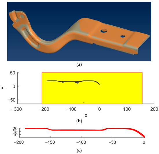
Figure 13. Comparison of the geometrical models (dimensions are represented in $\mathrm{m}\mathrm{m}$): (a) nominal vs. scanned model; (b) definition of the sectioning plane; (c) evaluation of the shapes of the nominal and scanned model.

3.4. Mapping Method of the Forming Simulation

Results from the simulation forming are available as a direct output. The file is structured, so the data is easily accessible for reading and analysis. Because adaptive meshing was enabled during the forming simulation, the number of elements increased significantly. Further simulation using the current numerical definition is difficult to implement and requires increased computational resources.

To overcome this issue, a user-defined MATLAB application was developed to map the results for different mesh sizes.

Figure 14a presents two sample meshes. On top, the current mesh used for simulation (receiving model) is shown. Behind is the mesh of the structure after the forming simulation (donor model). Figure 14b presents the thickness distribution after the forming simulation.

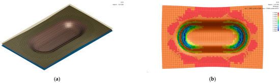
Figure 14. Mapping simulation results: (a) reference and forming meshes; (b) map of the thicknesses.

As a first step of the mapping process, the mesh definitions of the models are interpreted by the MATLAB application. For each finite element in the donor mesh, the coordinates of the centroid are determined as presented in equation set (3).

$$\begin{array}{c}{x}_{c,e}={\displaystyle \frac{1}{4}}\sum n_{i,x}\\ y_{c,e}={\displaystyle \frac{1}{4}}\sum n_{i,y}\\ z_{c,e}={\displaystyle \frac{1}{4}}\sum n_{i,z}\end{array}$$

(3)

The algorithm uses a 3D search domain to collect and average the input data. The 3D domain is defined by a parameter—search distance $s_d$—defined by the user. This parameter (Equation (4)) defines a cuboid with its center at the center of the finite element on the donor mesh.

$$\begin{array}{c}x\in \left[x_{c,e}-s_d\dots x_{c,e}+s_d\right]\\ y\in \left[y_{c,e}-s_d\dots y_{c,e}+s_d\right]\\ z\in \left[z_{c,e}-s_d\dots z_{c,e}+s_d\right]\end{array}$$

(4)

Based on this search zone, the elements from the donor model and the simulation results are collected. Results are averaged and associated with the current finite element of the receiving model (Equation (5)).

$$t_{e,ref}={\displaystyle \frac{1}{n_{e,s_d}}}\sum t_{e,dynain}$$

(5)

Figure 15 presents the results of the mapping algorithm for different values of the search distance.

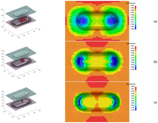
Figure 15. Results of the mapping method (dimensions are represented in $\mathrm{mm}$): (a) $s_d=10 \mathrm{mm}$; (b) $s_d=5 \mathrm{mm}$; (c) $s_d=2 \mathrm{mm}.$

Results presented in Figure 15 reveal that increasing the value of $s_d$ Parameter results are influenced by the average operator, as evidenced by the minimum thickness value. Therefore, the parameter $s_d$ should be selected with care, as local effects on the donor model may not be correctly transferred to the receiving model.

Figure 16 presents the mapping algorithm used for the mobile part. Thanks to the centroid-matching method, the mapping algorithm is robust; thus, it is not necessary to have a one–to–one matching of elements. This is the actual reason the forming simulation was finished after stage III.

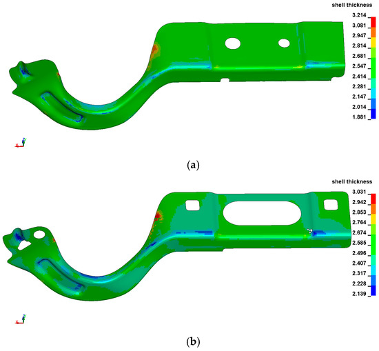
Figure 16. Results mapping for the mobile part: (a) forming analysis results; (b) model for structural analysis.

3.5. Results Mapping for 3D Elements

The structural analysis model is defined using 3D solid elements. Forming results are available for 2.5D shell elements. Therefore, the thickness associated with the shell elements must be converted to the dimensions of the 3D solid element. Figure 17a presents the definition of the finite elements for the middle surface [42].Two layers of solid elements are defined from the support surface as presented in Figure 17b. A layer is constructed in the positive direction of the normal, while the other is built in the negative direction. Figure 17c presents the 3D model with updated thickness.

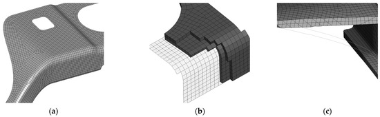
Figure 17. Numerical models: (a) mesh associated to the middle surface; (b) construction of the 3D solid elements; (c) updated 3D model.

To map the thickness determined from the forming analysis, it is necessary to update the dimensions of the 3D elements [43]. For each element, the edges that point toward the support surface are identified. The length of the edge is computed, and subsequently the components of the support vector of the edge (Equation (6)).

$$\begin{array}{c}{d}_{ij}=\sqrt{{\left(x_i-x_j\right)}^2+{\left(y_i-y_j\right)}^2+{\left(z_i-z_j\right)}^2}\\ \overline{i}={\displaystyle \frac{x_j-x_i}{d_{ij}}}\\ \overline{j}={\displaystyle \frac{y_j-y_i}{d_{ij}}}\\ \overline{k}={\displaystyle \frac{z_j-z_i}{d_{ij}}}\end{array}$$

(6)

The support vector is defined on the support surface. Using the thickness data stored by the shell element the length of the solid element is updated (Equation (7)).

$$\begin{array}{c}{x}_j^{\ast }=x_i+\overline{i}·t\\ y_j^{\ast }=y_i+\overline{i}·t\\ z_j^{\ast }=z_i+\overline{i}·t\end{array}$$

(7)

The elements’ residual stresses [44,45,46] determined after the forming simulation are exported via the ASCII file and associated with the 3D model. To simplify data processing, the results from the forming model, available for each through–thickness integration point, were averaged. The residual stresses are presented in Figure 18.

Figure 18. Residual stress: (a) results obtained from the forming simulation; (b) mapped data for the 3D model.

Mapping methods facilitate the use of various techniques and simulation results to develop detailed numerical models [47,48] capable of providing accurate results using reasonable resources.

4. Structural Performance Analysis

The numerical model developed to evaluate the structural performance of the assembly was created to mimic the fixtures used to support the actual parts during the experiments. Figure 19a shows the complete numerical model. The parts were clamped using a set of elements defined as rigids (*MAT_RIGID). The axes between the mobile and fixed parts were defined using joints (*CONSTRAINED_JOINT_REVOLUTE) as presented in Figure 19b. A very small amount of mobility is permitted at the bottom clamp of the testing machine. To account for the possibility of influencing the results, the clamp, modeled as a rigid body, was connected to the mobile part via a joint with a limited range of motion (*CONSTRAINED_JOINT_STIFFNESS_GENERALIZED). The load entry for the mobile part is located at the bolt holes.

Figure 19. The numerical model: (a) global view; (b) definition of the axes; (c) loading components.

The advantage of using the implicit solver is that the simulation time can be adapted to match the computational resources, without affecting the results (inertia).

4.1. Convergene Analysis

Previously, it was discussed that the hinge numerical model was built using two layers of 3D elements. To justify this approach, a convergence analysis was conducted. In Figure 20a, the reference model (RM) is shown. A simplified model (RM) with a single solid element through the thickness is illustrated in Figure 20b. The model is detailed with four elements through the thickness, as shown in Figure 20c. The number of solid elements through the thickness determines the overall size, as efforts are made during meshing to maintain cuboid shapes.

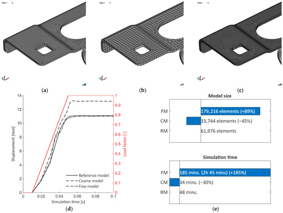
Figure 20. Convergence analysis: (a) Reference model—RM (two elements through thickness); (b) Coarse model—CM (one element through thickness); (c) Fine model—FM (four elements through thickness); (d) displacement plot; (e) performance plot.

Figure 20a presents the displacement history of the load entry sections. The load path is determined by the load factor parameter defined over the simulation time. The load factor determines multiple stages:

• − initialization with a value of zero;
• − loading when ramping from zero to one;
• − load keeping with a value of 0.

Initialization is required to apply gravity. During load ramping, the force is increased to the nominal value. The load-keeping stage is required to verify that no plastic hinges were formed. A constant value obtained during this stage indicated that the assembly can sustain the prescribed loads.

The displacement history shows that, in all cases, the solution converged. The maximum displacement recorded for the reference model is of $11.1 \mathrm{mm}$. The coarse model displays a value of $13.2 \mathrm{mm} \left(+19\%\right)$, while for the fine model, the results are identical to the reference model ($11.1 \mathrm{mm}$).

The performance analysis reveals that, for the model using two elements through thickness, a total of 61,976 elements is obtained. The number decreases for the coarse model to 33,744 ($-45\%$). The fine model requires an increased number of elements: 179,216 ($+89\%$). The number of elements in a numerical model determines the time required to obtain a solution. To solve the numerical model, an Intel i7-8086 (4 GHz) machine with 32 GB of RAM was used. The solver was set to implicit in the SMP (Shared Memory Parallel) model, and it was using 4 CPUs.

For the reference model, a runtime of 48 min was obtained, which decreased to 34 min $\left(-30\%\right)$ for the coarse model. The fine model required a runtime of 2 h and 45 min $\left(+185\%\right)$. The runtime is not directly proportional to the number of elements, as it also accounts for nonlinear behavior (interfaces and materials).

These results reveal that the solution of two elements through thickness is a reliable and efficient method for developing the numerical model.

4.2. Experimental vs. Numerical Analysis

A specialized fixture was constructed for the assembly to evaluate the performance under an axial force of $12 \mathrm{kN}$ corresponding to the load case High speed frontal crash (Figure 21).

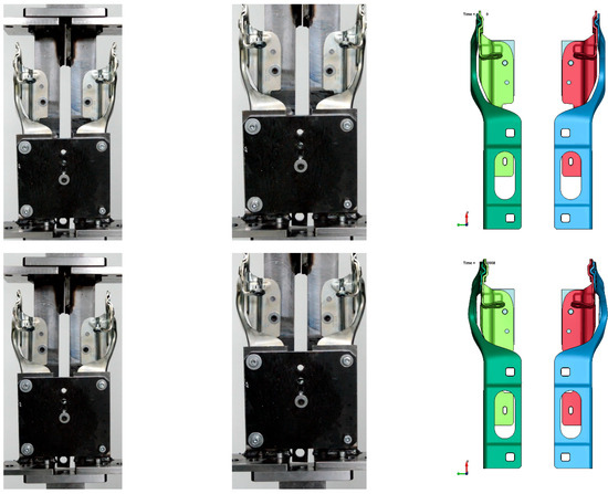
Figure 21. Experimental vs. simulation data (top—initial stage; bottom—final stage).

The experimental process was recorded using a digital camera [49]. The frames captured were processed to extract information related to the deformation of the structure [50,51,52]. Figure 22 illustrates the steps involved in processing the digital images.

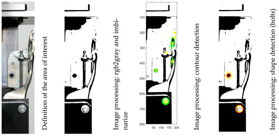
Figure 22. Digital image processing procedure: identification of the area of interest—conversion from RGB to grayscale and subsequently to black and white (binarize)—detection of contours (definition of a collection of edges)—detection of circular shapes (processing of edge information).

The algorithm used to detect the circular shapes from the collection of edges is defined by the equation set (8). The user corrects the selection of the shapes using the parameters $R_{min}$ and $R_{max}$.

$$\begin{array}{c}{x}_c={\displaystyle \frac{1}{n_p}}\sum x_i\\ y_c={\displaystyle \frac{1}{n_p}}\sum y_i\\ d_{i,\mathrm{c}}=\sqrt{{\left(x_i-x_c\right)}^2+{\left(y_i-y_c\right)}^2}\\ R_{min}\le d_{i,\mathrm{c}}\le R_{max}\end{array}$$

(8)

For each frame, the location of the bolts was detected. Figure 23a presents the coordinates of the circles with reference to the image definition (pixels), while Figure 23b presents the deformation of the structure during the loading process.

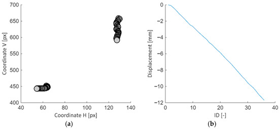
Figure 23. Digital image analysis: (a) image coordinates of the bolts; (b) deformation of the structure measured at the load entry.

5. Discussion

Three numerical models for the assembly were constructed. The first model–reference model–uses the nominal dimensions from the CAD file. For the second model, the finite elements were updated to capture the thickness changes resulting from the forming process. For the third model, both thickness changes and residual stress were included.

The loading history was extended with two additional stages: unloading, during which the load decreases to zero, and relaxation, to evaluate the residuals.

Figure 24a displays the displacement of the structure for each analysis case. As expected, the stiffest response is obtained for the model developed from the nominal model, with a maximum displacement of $11.1 \mathrm{mm}$. The thickness change has a minor influence on the results, with a maximum displacement of $11.4 \mathrm{mm}$ ($+2.7\%$). The full data mapping [53] shows an increase in the deformation of the structure [54] to $12.2 \mathrm{mm}$ ($+10\%$). This should be considered, as there is a load limit beyond which plastic hinges are developed, leading to the collapse of the structure.

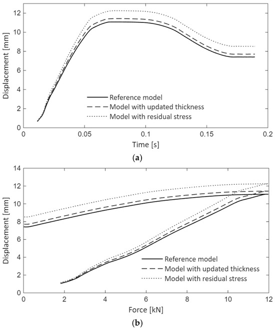
Figure 24. Results of the numerical simulation (history of the load entry): (a) displacement vs. simulation time; (b) displacement vs. load.

Figure 24b shows displacement vs. force (the primary parameter for this load case is the applied force). The plot provides an alternate view showing the displacement at peak load and residual deformation.

The simulation results are compared with the experimental data shown in Figure 25. During initial loading, the simulation model is stiffer than the experimental model. As the peak load is reached, the curves converge. The displacement recorded during the experiment is of $12.4 \mathrm{mm}$, while for the numerical model, a value of $12.2 \mathrm{mm}$ ($-1.6\%$) was obtained.

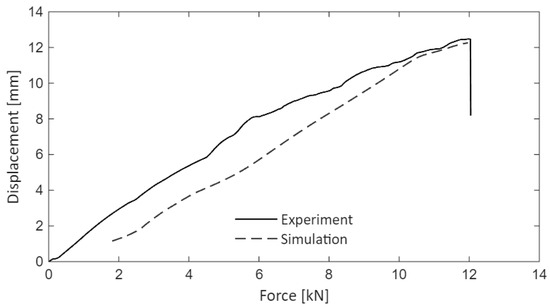
Figure 25. Experimental vs. numerical model–displacement at the load entry.

The stiffness of the testing machine and the fixture influences the behavior of experimental models during the initial loading stages.

A simple solution to improve the numerical model’s reliability while reducing computational effort is to define scale factors for different structural families, which are applied to the numerical model derived from the nominal definition.

$$s_{f,i}={\displaystyle \frac{d_{max}}{d_{max,ref}}}$$

(9)

The values of the scale factor as extracted from the results presented in Figure 24b are

$$\begin{array}{c}{s}_{f,1-2}={\displaystyle \frac{11.4}{11.1}}=1.03\\ s_{f,1-3}={\displaystyle \frac{12.2}{11.1}}=1.10\end{array}$$

(10)

1—Reference model; 2—Model with updated thickness; 3—Model with residual stresses

The applied force was scaled for the nominal model with a factor of $1.10$. The resulting displacement obtained from the simulation models is presented in Figure 26.

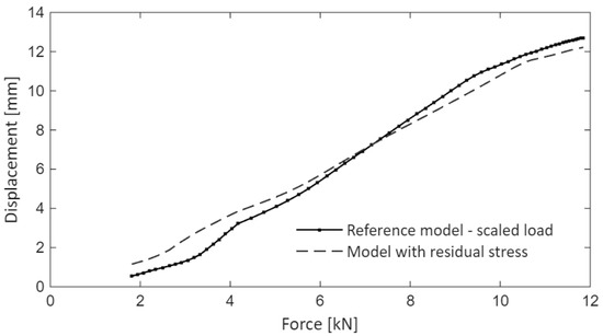
Figure 26. Simulation results (displacement at the load entry). Model with residual stresses vs. scaled model.

The maximum displacement for the model with scaled load ($13.2 \mathrm{kN}$) is of $12.7 \mathrm{mm}$, showing a slight increase of $4\%$ compared to the model with forming data, and a difference of $+2.4\%$ compared to the experiment.

The results from the scaled model agree with those from the model that includes residual stress.

6. Conclusions

In this work, a comprehensive analysis of a hood joint assembly was conducted. In this regard, the following stages were completed:

−

analysis of the assembly and identification of the constructive elements;

−

study of the technical specifications;

−

a synthesis of the constructive and technical elements and identification of the correlation method for meeting the operating requirements;

−

choice of material and mechanical characterization of the material;

−

the technological process of manufacturing the moving part component was researched, and semi-finished parts were taken after each stage;

−

the semi-finished parts corresponding to the stages of the technological process were investigated:

○

CAD models were created by 3D optical scanning;

○

a MATLAB application was developed that allows the geometric model to be aligned with the global reference;

○

CAD models of the scanned parts were compared with those obtained by numerical simulation of the manufacturing process.

−

a numerical model of the manufacturing process of the moving part was developed using the ANSYS Forming program:

○

the CAD model of the finished product was analyzed;

○

the stages of the numerical simulation process were developed in accordance with the stages of the technological process;

○

for each stage, significant results that influence the structural performance of the product were presented.

−

a numerical model of the product was developed to evaluate the structural performance:

○

the methods developed for processing the geometric model are presented;

○

the methods developed for creating the numerical model are presented;

−

through numerical simulation of the manufacturing process, information is obtained regarding the change in thickness of the part as well as the residual stress state resulting from the technological process:

○

a method was developed for transposing (mapping) the results obtained from the simulation of the technological process for the structural model;

○

a method was developed for creating the 3D finite element model for structural analysis that includes specific results of the technological process;

−

specific scenarios for numerical simulation were defined:

○

conventional model (reference);

○

variable thickness model (mapping);

○

residual stress model.

−

the physical assembly was experimentally investigated, and the results were processed using digital tools.

The experimental results were compared with simulation data, and a good correlation was identified, showing, for the numerical model with complete history (thickness and stress), a difference of $1.6\%$. However, this method requires multiple numerical models and an algorithm for results mapping, making this solution less feasible during the design stages.

To further simplify the numerical simulation process, a parameter is defined to scale the reference quantity, enabling the use of a conventional simulation model.

The determined scale factor can be applied to similar products, provided the manufacturing process follows a similar set of forming stages.

The work can serve as a benchmark for future complex simulations that integrate results from manufacturing processes. Moreover, it presents solutions for developing in-house data-exchange code.

References

- Giampieri, A.; Ling-Chin, J.; Ma, Z.; Smallbone, A.; Roskilly, A.P. A review of the current automotive manufacturing practice from an energy perspective. Appl. Energy 2020, 261, 114074. [Google Scholar] [CrossRef]
- Dalzochio, J.; Kunst, R.; Pignaton, E.; Binotto, A.; Sanyal, S.; Favilla, J.; Barbosa, J. Machine learning and reasoning for predictive maintenance in Industry 4.0: Current status and challenges. Comput. Ind. 2020, 123, 103298. [Google Scholar] [CrossRef]
- Bongomin, O.; Mwape, M.C.; Mpofu, N.S.; Bahunde, B.K.; Kidega, R.; Mpungu, I.L.; Tumusiime, G.; Owino, C.A.; Goussongtogue, Y.M.; Yemane, A.; et al. Digital twin technology advancing industry 4.0 and industry 5.0 across sectors. Results Eng. 2025, 26, 105583. [Google Scholar] [CrossRef]
- D’Avella, S.; Avizzano, C.A.; Tripicchio, P. ROS-Industrial based robotic cell for Industry 4.0: Eye-in-hand stereo camera and visual servoing for flexible, fast, and accurate picking and hooking in the production line. Robot. Comput.-Integr. Manuf. 2023, 80, 102453. [Google Scholar] [CrossRef]
- Al-Turjman, F.; Hussain, A.A.; Alturjman, S.; Altrjman, C. Vehicle Price Classification and Prediction Using Machine Learning in the IoT Smart Manufacturing Era. Sustainability 2022, 14, 9147. [Google Scholar] [CrossRef]
- Zhao, N.; Parthasarathy, M.; Patil, S.; Coates, D.; Myers, K.; Zhu, H.; Li, W. Direct additive manufacturing of metal parts for automotive applications. J. Manuf. Syst. 2023, 68, 368–375. [Google Scholar] [CrossRef]
- Hartley, W.D.; Garcia, D.; Yoder, J.K.; Poczatek, E.; Forsmark, J.H.; Luckey, S.G.; Dillard, D.A.; Yu, H.Z. Solid-state cladding on thin automotive sheet metals enabled by additive friction stir deposition. J. Mater. Process Technol. 2021, 291, 117045. [Google Scholar] [CrossRef]
- Douimia, S.; Bekrar, A.; Cadi, A.A.E.; Hillali, Y.E.; Fillon, D. Machine learning and deep learning applications in the automotive manufacturing industry: A systematic literature review and industry insights. Robot. Comput.-Integr. Manuf. 2025, 96, 103034. [Google Scholar] [CrossRef]
- Adnan Yusuf, S.; Khan, A.; Souissi, R. Vehicle-to-everything (V2X) in the autonomous vehicles domain–A technical review of communication, sensor, and AI technologies for road user safety. Transp. Res. Interdiscip. Perspect. 2024, 23, 100980. [Google Scholar] [CrossRef]
- Tihanyi, V.; Rövid, A.; Remeli, V.; Vincze, Z.; Csonthó, M.; Pethő, Z.; Szalai, M.; Varga, B.; Khalil, A.; Szalay, Z. Towards Cooperative Perception Services for ITS: Digital Twin in the Automotive Edge Cloud. Energies 2021, 14, 5930. [Google Scholar] [CrossRef]
- Fernandez De Arroyabe, I.; Watson, T.; Phillips, I. Cybersecurity Maintenance in the Automotive Industry Challenges and Solutions: A Technology Adoption Approach. Future Internet 2024, 16, 395. [Google Scholar] [CrossRef]
- Özmerdivanlı, A.; Sönmez, Y. The Relationship Between Financial Development, Energy Consumption, Economic Growth, and Environmental Degradation: A Comparison of G7 and E7 Countries. Economies 2025, 13, 278. [Google Scholar] [CrossRef]
- Palea, V.; Santhià, C. The financial impact of carbon risk and mitigation strategies: Insights from the automotive industry. J. Clean. Prod. 2022, 344, 131001. [Google Scholar] [CrossRef]
- Li, X.; Niu, W.; Tian, H. Application of Digital Twin in Electric Vehicle Powertrain: A Review. World Electr. Veh. J. 2024, 15, 208. [Google Scholar] [CrossRef]
- Ereiz, S.; Duvnjak, I.; Jiménez-Alonso, J.F. Review of finite element model updating methods for structural applications. Structures 2022, 41, 684–723. [Google Scholar] [CrossRef]
- Thacker, J.G.; Reagan, S.W.; Pellettiere, J.A.; Pilkey, W.D.; Crandall, J.R.; Sieveka, E.M. Experiences during development of a dynamic crash response automobile model. Finite Elem. Anal. Des. 1998, 30, 279–295. [Google Scholar] [CrossRef]
- Jayasinghe, S.C.; Mahmoodian, M.; Alavi, A.; Sidiq, A.; Shahrivar, F.; Sun, Z.; Thangarajah, J.; Setunge, S. A review on the applications of artificial neural network techniques for accelerating finite element analysis in the civil engineering domain. Comput. Struct. 2025, 310, 107698. [Google Scholar] [CrossRef]
- Yokoyama, Y.; Nagasaka, K.; Masuda, I.; Sugiyama, H.; Okazawa, S. Simulation of Automobile Structural Member Deformation and Crash via Isogeometric Analysis. Vehicles 2024, 6, 967–983. [Google Scholar] [CrossRef]
- Choi, S.; Park, T.; Kim, H.; Nam, B.; Ye, B.; Kim, D. Ductile fracture prediction in thin-walled structures through a novel damage model. Heliyon 2024, 10, e40849. [Google Scholar] [CrossRef]
- Abebe, M.; Koo, B. Fatigue Life Uncertainty Quantification of Front Suspension Lower Control Arm Design. Vehicles 2023, 5, 859–875. [Google Scholar] [CrossRef]
- Li, D.; Tian, J.; Shi, S.; Wang, S.; Deng, J.; He, S. Lightweight Design of Commercial Vehicle Cab Based on Fatigue Durability. CMES-Comput. Model. Eng. Sci. 2023, 136, 421–445. [Google Scholar] [CrossRef]
- Chen, S.; Bekar, E.T.; Bokrantz, J.; Skoogh, A. AI-enhanced digital twins in maintenance: Systematic review, industrial challenges, and bridging research–practice gaps. J. Manuf. Syst. 2025, 82, 678–699. [Google Scholar] [CrossRef]
- Suo, H.; Zhou, H.; Wei, Z.; Li, R.; Zhang, Y.; Guan, W.; Cheng, H.; Luo, B.; Zhang, K. Degradation mechanisms and mechanical behavior of composite-metal bolted/riveted joints in complex service conditions: A comprehensive review. Eng. Fail. Anal. 2025, 182, 110037. [Google Scholar] [CrossRef]
- Lv, X.; Xiao, Z.; Fang, J.; Li, Q.; Lei, F.; Sun, G. On safety design of vehicle for protection of vulnerable road users: A review. Thin-Walled Struct. 2023, 182, 109990. [Google Scholar] [CrossRef]
- Radu, A.-I.; Tolea, B.-A.; Trusca, D.-D. Validation of a virtual model for the kinematic and dynamic analysis of the impact of a pedestrian’s head with a bonnet using experimental tests. Ing. Automob. 2025. Available online: https://siar.ro/wp-content/uploads/2025/08/rIA_76.pdf (accessed on 2 October 2025).
- Abbasi, M.; Reddy, S.; Ghafari-Nazari, A.; Fard, M. Multiobjective crashworthiness optimization of multi-cornered thin-walled sheet metal members. Thin-Walled Struct. 2015, 89, 31–41. [Google Scholar] [CrossRef]
- Baroutaji, A.; Sajjia, M.; Olabi, A.G. On the crashworthiness performance of thin-walled energy absorbers: Recent advances and future developments. Thin-Walled Struct. 2017, 118, 137–163. [Google Scholar] [CrossRef]
- Isaac, C.W.; Duddeck, F. Current trends in additively manufactured (3D printed) energy absorbing structures for crashworthiness application–a review. Virtual Phys. Prototyp. 2022, 17, 1058–1101. [Google Scholar] [CrossRef]
- Jones, N. Structural Impact, 1st ed.; Cambridge University Press: Cambridge, UK, 1990; ISBN 978-0-521-30180-0. [Google Scholar]
- Stirosu, M.; Tabacu, S. Experimental and numerical analysis and validation of S460 steel. Univ. Pitesti Sci. Bull.-Automot. Ser. 2024, 34, 1–9. [Google Scholar] [CrossRef]
- Vormwald, M. Fatigue of Constructional Steel S460 under Complex Cyclic Stress and Strain Sequences. Procedia Eng. 2011, 10, 270–275. [Google Scholar] [CrossRef]
- Xu, T.H.; Zhang, L.M. Numerical implementation of a bounding surface plasticity model for sand under high strain-rate loadings in LS-DYNA. Comput. Geotech. 2015, 66, 203–218. [Google Scholar] [CrossRef]
- Woelke, P.B.; Londono, J.G.; Erhart, T.; Haufe, A.; Jurendic, S.; Anderson, D. Extension of the GISSMO fracture model for thin-walled structures under combined tensile and bending loads. Eng. Fract. Mech. 2024, 311, 110574. [Google Scholar] [CrossRef]
- Hallquist, J.O. LS-DYNA ® THEORY MANUAL. Available online: https://ftp.lstc.com/anonymous/outgoing/jday/manuals/ls-dyna_theory_manual_2006.pdf (accessed on 1 July 2025).
- Rust, W.; Schweizerhof, K. Finite element limit load analysis of thin-walled structures by ANSYS (implicit), LS-DYNA (explicit) and in combination. Thin-Walled Struct. 2003, 41, 227–244. [Google Scholar] [CrossRef]
- Arriaga, A.; Pagaldai, R.; Zaldua, A.M.; Chrysostomou, A.; O’Brien, M. Impact testing and simulation of a polypropylene component. Correlation with strain rate sensitive constitutive models in ANSYS and LS-DYNA. Polym. Test. 2010, 29, 170–180. [Google Scholar] [CrossRef]
- Narasimhan, N.; Lovell, M. Predicting springback in sheet metal forming: An explicit to implicit sequential solution procedure. Finite Elem. Anal. Des. 1999, 33, 29–42. [Google Scholar] [CrossRef]
- Kim, H.-K.; Kim, W.-J. A Springback Prediction Model for Warm Forming of Aluminum Alloy Sheets Using Tangential Stresses on a Cross-Section of Sheet. Metals 2018, 8, 257. [Google Scholar] [CrossRef]
- Ahmed, G.M.S.; Ahmed, H.; Mohiuddin, M.V.; Sajid, S.M.S. Experimental Evaluation of Springback in Mild Steel and its Validation Using LS-DYNA. Procedia Mater. Sci. 2014, 6, 1376–1385. [Google Scholar] [CrossRef][Green Version]
- Bénière, R.; Subsol, G.; Gesquière, G.; Breton, F.L.; Puech, W. A comprehensive process of reverse engineering from 3D meshes to CAD models. CAD Comput. Aided Des. 2013, 45, 1382–1393. [Google Scholar] [CrossRef]
- Amaral, R.L.; Neto, D.M.; Wagre, D.; Santos, A.D.; Oliveira, M.C. Issues on the Correlation between Experimental and Numerical Results in Sheet Metal Forming Benchmarks. Metals 2020, 10, 1595. [Google Scholar] [CrossRef]
- Gavalas, E.; Pressas, I.; Papaefthymiou, S. Mesh sensitivity analysis on implicit and explicit method for rolling simulation. Int. J. Struct. Integr. 2018, 9, 465–474. [Google Scholar] [CrossRef]
- Tabacu, S.; Ducu, C. Numerical investigations of 3D printed structures under compressive loads using damage and fracture criterion: Experiments, parameter identification, and validation. Extreme Mech. Lett. 2020, 39, 100775. [Google Scholar] [CrossRef]
- Acevedo, C.; Nussbaumer, A. Effect of tensile residual stresses on fatigue crack growth and S-N curves in tubular joints loaded in compression. Int. J. Fatigue 2012, 36, 171–180. [Google Scholar] [CrossRef]
- Hassani-Gangaraj, S.M.; Carboni, M.; Guagliano, M. Finite element approach toward an advanced understanding of deep rolling induced residual stresses, and an application to railway axles. Mater. Des. 2015, 83, 689–703. [Google Scholar] [CrossRef]
- Shang, D.; Liu, X.; Shan, Y.; Jiang, E. Research on the stamping residual stress of steel wheel disc and its effect on the fatigue life of wheel. Int. J. Fatigue 2016, 93, 173–183. [Google Scholar] [CrossRef]
- Varedi, S.R.; Buffel, B.; Desplentere, F. Post-forming deformation and thermal residual stress prediction in vacuum thermoformed ABS sheets. J. Manuf. Process 2025, 155, 1162–1170. [Google Scholar] [CrossRef]
- Sandin, O.; Larour, P.; Rodríguez, J.M.; Parareda, S.; Hammarberg, S.; Kajberg, J.; Casellas, D. Numerical modelling of shear cutting in complex phase high strength steel sheets: A comprehensive study using the Particle Finite Element Method. Finite Elem. Anal. Des. 2025, 246, 104331. [Google Scholar] [CrossRef]
- Liu, T.; Zheng, P.; Bao, J. Deep learning-based welding image recognition: A comprehensive review. J. Manuf. Syst. 2023, 68, 601–625. [Google Scholar] [CrossRef]
- Leonetti, D.; Baarssen, H.; Pucillo, G.P.; Snijder, B.H.H. Measurement of crack paths using digital image correlation. Eng. Fract. Mech. 2025, 327, 111391. [Google Scholar] [CrossRef]
- Almazán-Lázaro, J.-A.; López-Alba, E.; Díaz-Garrido, F.-A. Indentation measurement of thin plates using 3D digital image correlation and experimental validation. Results Eng. 2025, 25, 104246. [Google Scholar] [CrossRef]
- Li, D.; Cheng, B.; Shi, L.; Zhang, E.; Zhao, Q. Propagation measurement for visually thin fatigue crack using homography mapping error and digital image correlation. Mech. Syst. Signal Process 2024, 220, 111628. [Google Scholar] [CrossRef]
- Wang, S.; Wu, Y.; Xu, Q.; Ma, Y.; Wang, T. Research on stamping formability and process simulation of AZ31 magnesium alloy based on deep learning. Mater. Today Commun. 2024, 40, 109807. [Google Scholar] [CrossRef]
- Zeng, C.; Tian, W.; Liao, W.H. The effect of residual stress due to interference fit on the fatigue behavior of a fastener hole with edge cracks. Eng. Fail. Anal. 2016, 66, 72–87. [Google Scholar] [CrossRef]
Disclaimer/Publisher’s Note: The statements, opinions and data contained in all publications are solely those of the individual author(s) and contributor(s) and not of MDPI and/or the editor(s). MDPI and/or the editor(s) disclaim responsibility for any injury to people or property resulting from any ideas, methods, instructions or products referred to in the content. |
© 2025 by the authors. Licensee MDPI, Basel, Switzerland. This article is an open access article distributed under the terms and conditions of the Creative Commons Attribution (CC BY) license (https://creativecommons.org/licenses/by/4.0/).