IoT-Driven Destination Prediction in Smart Urban Mobility: A Comparative Study of Markov Chains and Hidden Markov Models

Abstract

The increasing availability of IoT-enabled mobility data and intelligent transportation systems in Smart Cities demands efficient and interpretable models for destination prediction. This study presents a comparative analysis between Markov Chains and Hidden Markov Models applied to urban mobility trajectories, evaluated through mean precision values. To ensure methodological rigor, the Smart Sampling with Data Filtering (SSDF) method was developed, integrating trajectory segmentation, spatial tessellation, frequency aggregation, and 10-fold cross-validation. Using data from 23 vehicles in the Vehicle Energy Dataset (VED) and a filtering threshold based on trajectory recurrence, the results show that the HMM achieved 61% precision versus 59% for Markov Chains (p = 0.0248). Incorporating day-of-week contextual information led to statistically significant precision improvements in 78.3% of cases for precision (95.7% for recall, 87.0% for F1-score). The remaining 21.7% indicate that model selection should balance model complexity and precision-efficiency trade-off. The proposed SSDF method establishes a replicable foundation for evaluating probabilistic models in IoT-based mobility systems, contributing to scalable, explainable, and sustainable Smart City transportation analytics.

1. Introduction

In the context of Smart Cities, where urban infrastructures are increasingly equipped with connected sensors and devices from the Internet of Things (IoT), mobility data have become a cornerstone for enhancing sustainability, safety, and traffic efficiency, according to [1]. The continuous collection of spatio-temporal data from vehicles, smartphones, and roadside units enables city administrators to monitor mobility patterns in real-time and design adaptive strategies for congestion management and energy optimization. However, extracting actionable insights from these heterogeneous IoT data streams remains challenging due to their volume, variability, and real-time constraints, according to [2]. In this scenario, developing lightweight and interpretable predictive models becomes essential to support intelligent transportation systems capable of anticipating user destinations and improving urban mobility decision-making.

To operationalize this vision of data-driven urban intelligence, the IoT relies on a dense network of sensing and communication devices embedded in vehicles, infrastructure, and personal equipment. These interconnected elements constitute the foundation of intelligent transportation systems, continuously capturing environmental and mobility-related information, as reported by [3,4]. Within the broader Internet of Vehicles (IoV) paradigm, recent advances leverage digital twin technology for real-time monitoring and resource management [5], enabling efficient task offloading and collaborative computing in vehicular edge networks. However, the increasing complexity of IoV infrastructures also introduces security challenges, including authentication attacks, data integrity threats, and availability concerns that must be addressed alongside predictive capabilities [6,7].

Considering this context, within the IoT domain, GPS receivers provide longitude, latitude, and timestamp data for each point (or vertex). By analyzing the continuity and spatio-temporal proximity of these vertices, it becomes possible to reconstruct the trajectories followed by a given object. Such trajectories enable the discovery of mobility patterns, including anomaly detection and habit inference. In this context, the importance of computational processing of spatio-temporal data collected by sensors becomes evident. As highlighted by [8], sensors play a fundamental role in these systems, as they gather relevant information from cities, citizens, and communication networks that transmit data in real-time.

Patterns derived from trajectories also support practical applications by facilitating the definition of alternative routes in the presence of obstructions or habit changes, while enabling the identification of origin–destination flows, which assist in managing traffic segments and periods of congestion, as reported by [9]. Recent advances highlight the importance of transparent and explainable models not only for fairness in decision systems, according to [10], but also for interpretability in predictive analytics. In this context, probabilistic approaches such as Markovian frameworks remain valuable for ensuring explainability while maintaining computational efficiency. By combining computational methods with sensing technologies, it becomes possible not only to identify faster or safer routes for individual users but also to provide comprehensive and context-aware insights for traffic management teams in Smart Cities.

However, effective destination prediction within IoT-enabled mobility systems necessitates methodologies that reconcile predictive accuracy with computational efficiency. This challenge is particularly relevant when deploying embedded GPS receivers integrated with energy and speed monitoring sensors in urban passenger vehicles, where resource constraints demand lightweight architectures suitable for edge computing environments. Probabilistic frameworks such as Markov Chains [11] and Hidden Markov Models (HMMs) [12] offer computationally tractable approaches for capturing sequential dependencies in mobility patterns. Nevertheless, the predictive performance of such models is contingent upon judicious sample selection strategies. This is especially critical when filtering trajectories according to temporal attributes and recurrence frequencies. Furthermore, prevailing methodologies often reduce trajectory representation to origin–destination pairs. Such simplification potentially disregards intermediate waypoints that may convey contextual information.

Despite significant advances in trajectory prediction using deep learning and hybrid approaches, few studies have systematically compared purely probabilistic frameworks under real-world IoT mobility constraints. Recent comprehensive surveys emphasize that while deep learning methods achieve high accuracy, they often lack interpretability and require substantial computational resources, factors that hinder their deployment in embedded IoT environments. Moreover, limited research exists for datasets that couple GPS-derived trajectories with vehicular performance metrics such as energy consumption and speed profiles. Recent work on region-level traffic prediction [13] and urban mobility pattern detection [14] demonstrates the value of GPS-based trajectory analysis, yet comprehensive evaluations comparing Markovian frameworks remain scarce. In particular, the literature lacks comprehensive evaluations of how contextual temporal variables, such as day of the week or trip recurrence, affect the predictive performance of Markovian models. This gap highlights the need for transparent and statistically grounded analyses that can reveal the trade-offs between model interpretability, computational efficiency, and prediction accuracy in IoT-driven transportation systems.

Within this scenario, destination prediction assumes a central role. Anticipating the probable destination of the user contributes to the efficiency of urban traffic systems while offering convenience to drivers and passengers [13]. Moreover, destination prediction can incorporate factors beyond spatio-temporal data, such as carbon emission control, energy consumption, and the detection of speed-related patterns along specific routes. These aspects guide the future redesign of traffic signals in particular segments. Furthermore, the findings provide actionable insights for developing lightweight, interpretable mobility prediction systems deployable on embedded IoT devices within Smart City infrastructures.

Despite significant advances in trajectory prediction using deep learning and hybrid approaches, few studies have systematically compared purely probabilistic frameworks under real-world IoT mobility constraints. Deep learning methods, while achieving high accuracy, demand substantial computational resources that frequently exceed the capabilities of resource-constrained edge devices [15], limiting their practical deployment in embedded IoT environments. This limitation reveals a critical gap in understanding how contextual temporal variables, such as trip recurrence and day of the week, influence predictive outcomes in Markovian models. Addressing this gap is essential for developing lightweight, explainable, and computationally feasible prediction systems that can operate within vehicular IoT infrastructures in Smart Cities. In response, this work proposes a transparent and statistically grounded framework that systematically compares Markov Chains and Hidden Markov Models using real-world vehicular IoT data, as detailed in the following contributions.

1.1. Contributions

This work makes the following contributions to the field of vehicular trajectory prediction in IoT environments:

• Development of destination predictors based on Markov Chains and Hidden Markov Models, systematically compared through inferential statistical testing (Student’s t-test) across 23 passenger vehicles;
• Introduction of the Smart Sampling with Data Filtering (SSDF) methodology for trajectory preprocessing, which selects recurrent patterns based on temporal features and frequency thresholds from real-world publicly available data (Vehicle Energy Dataset);
• Comprehensive multi-metric evaluation (Precision, Recall, F1-score) with 10-fold cross-validation, revealing critical trade-offs between precision and coverage in Markovian frameworks that single-metric studies typically overlook;
• Demonstration that transparent probabilistic models can achieve competitive performance while maintaining interpretability and computational tractability, essential requirements for deployment on resource-constrained vehicular IoT devices in Smart Cities.

1.2. Organization

The remainder of this paper is organized as follows. Section 2 reviews the related works on trajectory prediction and destination forecasting, based on a Systematic Literature Mapping (SLM) that identified 33 studies addressing predictive models for trajectories and destinations. Section 3 provides the theoretical background on Markov-based frameworks. Section 4 presents the proposed Smart Sampling with Data Filtering (SSDF) method. Section 5 describes the experimental setup and presents the results. Section 6 discusses the findings and their implications. Finally, Section 7 concludes the paper and suggests future research directions.

2. Related Works

This study was grounded in a Systematic Literature Mapping (SLM) conducted following the protocol proposed by [16]. The process involved defining research questions, selecting relevant databases (including ACM, IEEE, and MDPI), and applying inclusion and exclusion criteria to identify works related to trajectory and destination prediction. Studies published between 2017 and 2023 were considered, covering diverse approaches such as deep learning, clustering, hybrid, and probabilistic methods. After applying quality filters and full-text screening, 33 papers were selected for detailed analysis. This mapping provided an overview of methodological trends and revealed a noticeable lack of studies performing direct statistical comparisons between probabilistic models, particularly Markov Chains and Hidden Markov Models, within IoT-based mobility contexts [17].

This process enabled an analysis of the SLM landscape, delineating predictions employing clustering techniques, such as hierarchical clustering approaches; deep neural networks, exemplified by convolutional architectures; Markovian models, as demonstrated by temporal Markov frameworks; and hybrid algorithms integrating multiple methods, such as Kalman filters combined with Long Short-Term Memory (LSTM) networks. However, a notable gap was identified regarding pure Markovian techniques; that is, approaches not combined with more recent methods. Furthermore, there was an absence of foundational analyses examining how and to what extent contextual factors influence model accuracy, suggesting the need to mitigate these effects through appropriate sampling strategies.

The studies identified in the SLM span diverse methodological approaches. Of the 33 articles initially selected, seven of them were identified as most pertinent to the scope of this study and are summarized in Table 1. Selection criteria prioritized either temporal relevance (publications proximate to 2025) or methodological alignment with Markovian frameworks for destination prediction. A detailed comparative analysis distinguishing these works from the present study is provided in Table 2. Unlike most recent trajectory prediction studies that emphasize deep learning or neural approaches, this work focuses on probabilistic and statistically interpretable models. Few prior works have systematically compared Markov Chains and Hidden Markov Models under controlled sampling and data balancing conditions, which creates a gap in understanding how contextual variables, such as day of the week, affect predictive performance. This distinction motivates the comparative framework proposed in this study.

Table 1 organizes the selected studies according to the following descriptors: authorship and publication year; multi-scenario data usage, denoted by Y (Yes) when multiple data sources or experimental scenarios were employed, or N (No) otherwise; prediction scope, classified as collective (C) when addressing aggregate mobility patterns, individual (I) when focusing on single-user trajectories, or both (B); spatial context, categorized as urban (U) environments or other contexts (O); and the computational methods or predictive frameworks adopted in each study.

Depending on the article, greater emphasis was placed on computational performance or methodological aspects. For example, Ref. [18] analyzed the ability of their algorithm to process data in real-time, while Ref. [19] focused on the predictive precision of the proposed model, validated by Root Mean Squared Error (RMSE).

Table 1. Comparison of related works.

Citation	Type	Mode	Method	Algorithms/Techniques
Dai et al., 2019 [20]	Y	I	U	ST-LSTM (Spatio-Temporal LSTM)
Lassoued, 2017 [21]	Y	C	O	Simplified HMM with clustering
Sadri et al., 2018 [19]	Y	I	U	TrAF (Trajectory Affinity)
Qin et al., 2023 [22]	N	C	U	UTA (Urban Topology-encoding Spatiotemporal Attention Network)
Santana and Campos, 2017 [23]	N	I	O	Semantic approach with social interactions
Shen et al., 2023 [24]	S	I	U	STI-GCN (Spatio-Temporal Interactive Graph Convolutional Network), CNN
Wang et al., 2023 [18]	Y	I	U	Transformer-based model with IoT

Table 1. Comparison of related works.

Citation	Type	Mode	Method	Algorithms/Techniques
Dai et al., 2019 [20]	Y	I	U	ST-LSTM (Spatio-Temporal LSTM)
Lassoued, 2017 [21]	Y	C	O	Simplified HMM with clustering
Sadri et al., 2018 [19]	Y	I	U	TrAF (Trajectory Affinity)
Qin et al., 2023 [22]	N	C	U	UTA (Urban Topology-encoding Spatiotemporal Attention Network)
Santana and Campos, 2017 [23]	N	I	O	Semantic approach with social interactions
Shen et al., 2023 [24]	S	I	U	STI-GCN (Spatio-Temporal Interactive Graph Convolutional Network), CNN
Wang et al., 2023 [18]	Y	I	U	Transformer-based model with IoT

Table 2. Comparative analysis of articles in relation to the proposed work.

Authors	Model	Data Context	Validation	Unique Contribution
Wang et al., 2023 [18]	Transformer-based model	Argoverse dataset	Minimum Average Displacement Error (minADE) and Minimum Final Displacement Error (minFDE)	Real-time online inference using IoT computational resources
Sadri et al., 2018 [19]	Trajectory Affinity (TrAF) based on similarity between trajectory segments	Device Analyzer (cell towers) vs. Mobile Data Challenge (GPS + WLAN)	RMSE comparison between techniques	Simplicity and long-term focus, considering residence and departure times, correlation between morning and evening trajectories
Dai et al., 2019 [20]	Spatio-Temporal LSTM (ST-LSTM)	I-80 and US-101 datasets (NGSIM)	RMSE comparison with baseline Maneuver LSTM (M-LSTM)	Joint modeling of spatial interactions and temporal relations for long time series; includes shortcut connections to mitigate gradient vanishing
Lassoued, 2017 [21]	Simplified HMM with clustering by destination points	City of Dublin through OpenStreetMap and SUMO simulation	Convergence rate based on number of road links needed for correct prediction	Clustering historical driver trips into groups with similar patterns
Santana and Campos, 2017 [23]	Semantic approach combining positioning with social interactions	Raw Trajectory Data (RTD), Semantic Trajectory, and Georeferenced Social Interactions (GSI)	Accuracy	Multi-source data integration and use of semantic information
Shen et al., 2023 [24]	Spatio-Temporal Interactive Graph Convolutional Network (STI-GCN)	I-80 and US-101 datasets from NGSIM	Number of parameters and inference time	Holistic approach for autonomous driving; CNN for temporal feature extraction; captures dynamic vehicle interactions
Qin et al., 2023 [22]	Urban Topology-encoding Spatiotemporal Attention Network (UTA)	Proprietary taxi dataset from Hangzhou, China	AUC, Group AUC (GAUC), ROC	Urban topological network construction, GPS mapping, semantic information attachment, and topological graph encoding

Table 2. Comparative analysis of articles in relation to the proposed work.

Authors	Model	Data Context	Validation	Unique Contribution
Wang et al., 2023 [18]	Transformer-based model	Argoverse dataset	Minimum Average Displacement Error (minADE) and Minimum Final Displacement Error (minFDE)	Real-time online inference using IoT computational resources
Sadri et al., 2018 [19]	Trajectory Affinity (TrAF) based on similarity between trajectory segments	Device Analyzer (cell towers) vs. Mobile Data Challenge (GPS + WLAN)	RMSE comparison between techniques	Simplicity and long-term focus, considering residence and departure times, correlation between morning and evening trajectories
Dai et al., 2019 [20]	Spatio-Temporal LSTM (ST-LSTM)	I-80 and US-101 datasets (NGSIM)	RMSE comparison with baseline Maneuver LSTM (M-LSTM)	Joint modeling of spatial interactions and temporal relations for long time series; includes shortcut connections to mitigate gradient vanishing
Lassoued, 2017 [21]	Simplified HMM with clustering by destination points	City of Dublin through OpenStreetMap and SUMO simulation	Convergence rate based on number of road links needed for correct prediction	Clustering historical driver trips into groups with similar patterns
Santana and Campos, 2017 [23]	Semantic approach combining positioning with social interactions	Raw Trajectory Data (RTD), Semantic Trajectory, and Georeferenced Social Interactions (GSI)	Accuracy	Multi-source data integration and use of semantic information
Shen et al., 2023 [24]	Spatio-Temporal Interactive Graph Convolutional Network (STI-GCN)	I-80 and US-101 datasets from NGSIM	Number of parameters and inference time	Holistic approach for autonomous driving; CNN for temporal feature extraction; captures dynamic vehicle interactions
Qin et al., 2023 [22]	Urban Topology-encoding Spatiotemporal Attention Network (UTA)	Proprietary taxi dataset from Hangzhou, China	AUC, Group AUC (GAUC), ROC	Urban topological network construction, GPS mapping, semantic information attachment, and topological graph encoding

In [18], the Lane Transformer, a deployment-oriented architecture that replaces Graph Convolutional Networks (GCNs) with multi-head attention blocks for trajectory prediction, was introduced. Trained on the Argoverse dataset, their model employs a four-stage pipeline: vectorization preprocessing of trajectories and HD maps, attention-based scene context encoding, hierarchical transformer fusion blocks for local and global interactions, and MLP-based (Multi-Layer Perceptron) multi-modal trajectory generation. Performance evaluation utilized minADE (measuring average Euclidean distance across all predicted timesteps) and minFDE (assessing final endpoint accuracy). The architecture’s key innovation lies in its TensorRT-compatible design, achieving 7 ms inference time, a 10× to 25× speedup over the baseline LaneGCN, while maintaining comparable accuracy (minADE: 0.86, minFDE: 1.31). This breakthrough in efficiency enables real-time deployment on edge vehicular computing platforms within IoT-enabled intelligent transportation systems.

Meanwhile, Ref. [19] addressed the continuous trajectory prediction problem by leveraging behavioral patterns and temporal correlations in human mobility. Their Trajectory Affinity (TrAF) method measures similarity between trajectory segments using a combination of Dynamic Time Warping (DTW) and Edit Distance metrics. The approach was validated on two datasets: Device Analyzer (cell tower data) and Mobile Data Challenge (GPS + WLAN), with the latter providing more realistic mobility patterns through multi-source positioning. The method’s key innovation lies in correlating morning and evening trajectories to predict afternoon movements, incorporating residence times, departure patterns, and temporal segmentation. By identifying similar historical sub-trajectories and removing outliers, TrAF achieved 10–35% error reduction compared to baselines (RMSE measured by DTW), demonstrating the effectiveness of exploiting daily routine patterns for long-term trajectory prediction.

The work of [23], which also focused on behavioral dynamics, introduced semantic and social interaction data. The authors utilized Raw Trajectory Data (RTD), Semantic Trajectories, and Georeferenced Social Interactions (GSI). A distinctive feature of this work is its independence from a single data source and the integration of semantic information. User positioning was combined with social interactions, and performance was measured using accuracy.

Other works concentrated primarily on technical innovations. For example, Ref. [24] proposed a Spatio-Temporal Interactive Graph Convolutional Network (STI-GCN), tested on the I-80 and US-101 datasets from NGSIM. Their method targeted autonomous driving, incorporating temporal variables extracted with Convolutional Neural Networks (CNNs). This enabled the capture of dynamic interactions among vehicles. However, the evaluation methods were less explicit, with only model parameters and inference time reported.

The work by [21] focused on clustering historical driver trips in Dublin using OpenStreetMaps and Simulation of Urban MObility (SUMO). Trips were grouped by destination points, and a simplified HMM was applied to detect route patterns. The evaluation metric utilized was the convergence rate, defined by how quickly the algorithm predicted the correct route based on the number of road links.

In the study by [20], the I-80 and US-101 datasets (NGSIM) were also employed. The authors proposed a Spatio-Temporal Long Short-Term Memory (ST-LSTM) network, designed to capture both spatial and temporal dependencies. Performance was evaluated with RMSE, comparing ST-LSTM against the state-of-the-art Maneuver LSTM (M-LSTM). Results demonstrated that ST-LSTM achieved lower prediction error than M-LSTM.

Finally, Ref. [22] introduced the Urban Topology-encoding Spatiotemporal Attention Network (UTA). Their model combines urban topological network construction, GPS mapping, semantic information attachment, and graph encoding. The dataset consisted of taxi trajectories collected in Hangzhou, China. Evaluation was conducted using the Area Under Curve (AUC), Group AUC (GAUC), and Receiver Operating Characteristic (ROC) metrics. UTA was also compared with baseline models, including HMM, RNN, LSTM, and Transformers.

In summary, these studies reflect three main perspectives: (i) human mobility behavior, (ii) technical and methodological advances, and (iii) computational performance. While many works achieved strong results in their respective domains, they generally lack a pipeline capable of generating appropriately sampled datasets for predictive algorithms, which constitutes the focus of this work.

Table 2 provides a comparative analysis distinguishing the reviewed literature from the present study. The fields include: identification of Authors (references), the Model employed, the Data Context (origin and characteristics of the datasets, whether real or synthetic, or cases where such information is absent), the Validation techniques applied, and the Unique Contributions of each study, which serve as points of reference for this research.

Unlike the majority of recent neural-based trajectory predictors, the proposed SSDF method emphasizes statistical transparency and reproducibility. This enables a fair comparison between stochastic models such as Markov Chains and Hidden Markov Models, highlighting under which sampling and contextual conditions each approach performs best. The novelty of this work therefore lies not only in the methodological pipeline itself, but also in establishing a replicable statistical foundation for model comparison within IoT-based mobility datasets.

The most relevant distinctions of our work lie in three key contributions: the novel sampling procedure, the data balancing strategy, and the comprehensive methodological pipeline integrating these components. These elements collectively proved essential for improving predictive performance. Additionally, this study employs a real and relatively recent dataset: the Vehicle Energy Dataset (VED).

Unlike prior works that rely mainly on RMSE, AUC, or displacement-based metrics, Precision was selected as the primary validation metric. This choice was made because Precision directly reflects the accuracy of correctly predicted destinations. It provides a more interpretable and application-oriented measure for Intelligent Transportation Systems. The metric aligns the evaluation with real-world scenarios in which decision-making depends on identifying the correct endpoint rather than minimizing spatial error alone. Furthermore, Precision enables assessment of the conditions under which one model can outperform another when contextual information is incorporated.

Beyond trajectory prediction methodologies, the broader IoV ecosystem presents complementary research challenges that contextualize the operational environment for predictive systems. Recent surveys have systematically examined security vulnerabilities inherent to IoV infrastructures, identifying critical threats in both intra-vehicular and inter-vehicular communications that compromise data confidentiality, integrity, and availability [25]. These security concerns are particularly relevant when deploying prediction models in distributed vehicular networks, as compromised sensor data directly undermines the reliability of trajectory inference. Concurrently, advances in vehicular edge computing have explored blockchain-based architectures combined with digital twin technology to address computational offloading challenges while maintaining security in resource-constrained environments [26]. Such infrastructural considerations, although not the primary focus of this comparative study, underscore the importance of developing lightweight probabilistic models capable of operating reliably within the security and computational constraints characteristic of real-world IoV deployments. The present work addresses this need by focusing specifically on the statistical comparison of Markovian frameworks under controlled sampling conditions, providing a foundation for transparent and reproducible trajectory prediction that can be integrated into broader IoV systems.

This section concludes by noting that only a subset of the works identified through the SLM process were detailed here, owing to space limitations. Nonetheless, the discussion highlights the particularities of each model and dataset and their relationship with this research. While many relevant studies on clustering techniques and deep neural networks exist, the focus of this work is to provide a meaningful comparison between Markovian models. This comparison evaluates their effectiveness in destination prediction.

In summary, the reviewed approaches demonstrate significant progress in trajectory and destination prediction. However, none of them provide a unified statistical pipeline that enables reproducible comparison between probabilistic models under controlled sampling conditions. This gap reinforces the need for a transparent and systematic method. Such a method should be capable of revealing how contextual and temporal variables influence predictive performance. The following section presents the theoretical background, establishing the conceptual foundation for the proposed method to handle locational sensor data.

3. Background

To implement the predictive models presented in this work, it is essential to understand the types of spatio-temporal and semantic data, as well as the methods used to represent and process urban space. These concepts lay the foundation for trajectory modeling, sampling, and the use of Markov-based prediction techniques.

Spatial data encode both geometric properties and semantic attributes, which are processed through Geographic Information Systems (GIS) that provide computational frameworks for spatial analysis and visualization. Geographic data positioning relies on Coordinate Reference Systems (CRS), which define mathematical transformations for representing Earth’s curved surface on planar coordinates, ensuring accurate spatial referencing [27].

Temporal attributes utilize standardized datetime formats, predominantly Coordinated Universal Time (UTC), which ensures temporal consistency and interoperability across distributed IoT sensor networks and transportation systems [8]. This temporal standardization is essential for synchronizing spatio-temporal data collected from multiple sensors and devices in urban mobility applications.

Semantic enrichment augments raw spatio-temporal trajectories with contextual attributes, such as day of week, temporal periods, activity types, or environmental conditions, enabling trajectory interpretation beyond geometric coordinates alone [28,29]. This semantic layer facilitates pattern recognition and behavioral analysis in urban mobility contexts.

As illustrated in Figure 1, spatial tessellation partitions geographic regions into discrete cells through systematic grid structures, facilitating computational analysis of spatial phenomena and movement patterns [30,31]. Voronoi tessellations (also termed Thiessen polygons) construct partitions where each cell contains points nearest to a specific generator location, providing optimal spatial subdivisions for proximity-based analyses [32].

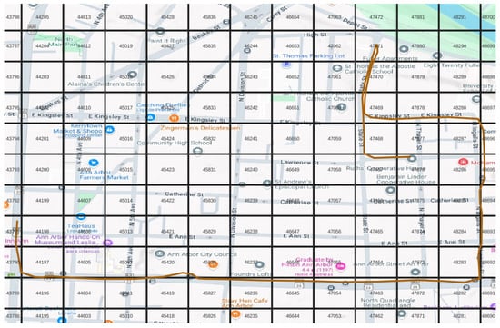
Figure 1. Example of a tessellated grid.

By understanding these data types and techniques, it becomes possible to represent geographic coordinates as discrete states (e.g., cells $⟨100⟩$, $⟨201⟩$, $⟨960⟩$) that can be incorporated into Markov Chains.

Origin–Destination (OD) pairs encode trajectory endpoints as discrete grid identifiers, where each trajectory $\tau$ is characterized by its starting location (origin) and terminal location (destination), forming the basis for aggregate flow analysis in transportation systems [33]. For instance, a trajectory labeled $⟨150,170⟩$ indicates a movement from cell 150 (origin) to cell 170 (destination). Predictive modeling focuses on determining the destination cell from the observed origin.

Trajectory segmentation decomposes continuous movement traces into semantically coherent sub-trajectories through various algorithmic approaches: feature-based classification, temporal interpolation, density-based clustering, or stay-point detection [28,34]. Stay-point detection algorithms identify spatio-temporal regions where movement velocity falls below defined thresholds, enabling trajectory partitioning into stationary and mobile phases, a fundamental preprocessing step for mobility pattern analysis [35,36]. Once trajectories are appropriately segmented and represented as sequences of origin–destination transitions, probabilistic frameworks can be applied to model movement patterns and predict future destinations.

3.1. Markov Chain Models for Sequential Prediction

In probability distributions, current data influences only the immediately subsequent data point, with no effect on further successive points.

Markov models capture probabilistic patterns in spatial transitions: if a user visits “home” on N occasions and subsequently visits “park” with measurable frequency, this pattern demonstrates repetition according to determinable probabilities. Consider five discrete spatial states representing traffic zones A–E (where A represents home and B represents park). These states function as origins and destinations within sub-trajectories. Among the five states, transitions encode probabilistic movements between them. Note that a transition from grid cell A to B represents a vehicle moving between two traffic zones within the city, while the transition probability reflects the likelihood of this movement occurring.

For illustration, consider the transition probabilities from state A: directly to B with probability 0.3; to C with probability 0.2; to D with probability 0.1; and to E with probability 0.4. These probabilities sum to unity: $0.3+0.2+0.1+0.4=1$, satisfying the row-stochastic constraint. In this particular example (Table 3), diagonal elements are zero, indicating that immediate self-transitions are not permitted, vehicles must move to different zones at each time step.

Figure 2 visualizes the state transition structure, while Table 3 provides the complete transition probability matrix, labeled as symbol P. Each alphabetical designation represents discretized geographical coordinates that, through tessellation procedures, have been transformed into traffic analysis zones. No latent factors are presumed to interfere with transition probability values.

When implementing Markov Chains for trajectory prediction, the selection of appropriate sample filtration thresholds during data preparation remains crucial [37]. A Markov Chain model requires achieving equilibrium between sufficient data retention for statistical reliability and avoiding excessive sparsity that undermines estimation quality.

Figure 2. First-order Markov Chain model with five-state transition structure [38].

Table 3. Transition probability matrix P for the five-state Markov chain model. Matrix elements $p_{ij}$ represent the probability of transitioning from state i to state j, where ${\sum }_j{p}_{ij}=1$ for all i [39].

From/To	A	B	C	D	E
A	0.0	0.3	0.2	0.1	0.4
B	0.1	0.0	0.4	0.2	0.3
C	0.3	0.2	0.0	0.1	0.4
D	0.2	0.3	0.4	0.0	0.1
E	0.2	0.3	0.1	0.4	0.0

Table 3. Transition probability matrix P for the five-state Markov chain model. Matrix elements $p_{ij}$ represent the probability of transitioning from state i to state j, where ${\sum }_j{p}_{ij}=1$ for all i [39].

From/To	A	B	C	D	E
A	0.0	0.3	0.2	0.1	0.4
B	0.1	0.0	0.4	0.2	0.3
C	0.3	0.2	0.0	0.1	0.4
D	0.2	0.3	0.4	0.0	0.1
E	0.2	0.3	0.1	0.4	0.0

3.2. Hidden Markov Models with Contextual Information

Note, HMMs are particularly suitable for IoT-based mobility data because they can capture stochastic dependencies in trajectories while incorporating contextual temporal features without requiring deep architectures [40]. Hidden Markov Models extend this framework by encompassing not only the relationship with destinations, but also the Viterbi algorithm and the concept of “hidden” states inherent in the model nomenclature. Initially, considering hidden factors beyond those included in a transition probability matrix, with their own “emission” probabilities involved, it becomes possible to exemplify a path or journey through sub-trajectories, as represented in Figure 3.

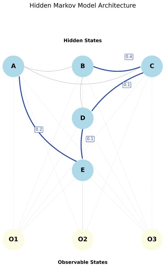
Figure 3. Hidden Markov Model architecture showing hidden states (A–E) and observable states (O1–O3).

In this sense, states A, B, C, D, and E initially follow the same logic as a standard Markov Chain, representing discrete spatial locations (traffic analysis zones). However, in Hidden Markov Models, the term “hidden” derives from the fact that these states, the actual origin locations, are treated as latent variables. What makes them “hidden” is that the model incorporates observable contextual information, specifically “day of the week,” to condition the predictions. These observable features are represented as symbols (O1, O2, O3 in Figure 4, corresponding to Monday, Wednesday, and Friday).

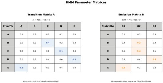
Figure 4. HMM parameter matrices estimated via Maximum Likelihood Estimation. The transition matrix $\mathbf{A}$ (left) contains state transition probabilities $a_{ij}$, computed by counting transitions between origin locations and normalizing by row. The emission matrix $\mathbf{B}$ (right) shows emission probabilities $b_i\left(k\right)$, representing the likelihood of observing each weekday from each origin state. Highlighted paths demonstrate Viterbi decoding examples.

The framework operates as follows: if a vehicle originates from location A (hidden state) and the contextual observation indicates it is Friday (symbol O3), the model uses both the transition probabilities between locations and the emission probabilities linking locations to weekdays to predict the destination. For instance, suppose the emission matrix shows that departures from state A occur with higher probability on Fridays (e.g., $b_A\left(\mathrm{Friday}\right)=0.5$), while the transition matrix indicates that vehicles leaving A tend to move to state C with probability $a_{AC}=0.4$. The HMM combines these two sources of information, spatial transition patterns and temporal context, to predict that destination C is likely when departing from A on a Friday.

This research focuses specifically on this integration of spatial transitions with a single temporal feature (day of week). The model does not incorporate additional complexity such as time of day, traffic conditions, or other contextual variables. The objective is to understand how incorporating weekday information through the emission matrix improves destination prediction compared to standard Markov Chains that rely solely on spatial transition patterns.

The emission matrix $\mathbf{B}$ relates hidden states (origin locations) to observations (days of the week). In this example, three observation symbols, “O1,” “O2,” and “O3”, represent Monday, Wednesday, and Friday, respectively. Each element $b_i\left(k\right)=P\left(O_k\right|S=i)$ denotes the emission probability of observing weekday k from hidden state i, as illustrated in Figure 4.

Both matrices are learned from training data using Maximum Likelihood Estimation [41,42], with probabilities computed as normalized counts: $a_{ij}=C(i\to j)/{\sum }_{k}C(i\to k)$ for transitions and $b_i\left(k\right)=C(S=i,O=k)/{\sum }_{m}C(S=i,O=m)$ for emissions, where $C(·)$ where $n_{ij}$ denotes the count of transitions from state i to state j, and $m_k\left(i\right)$ represents the count of symbol k observed from state i. This dual-matrix structure enables HMMs to incorporate both spatial transition patterns and temporal contextual information, here, the day of the week, into destination predictions [43]. While this implementation focuses on weekday patterns, the framework extends naturally to other temporal features such as time of day or traffic conditions.

The Viterbi algorithm provides the computational mechanism for HMM decoding, efficiently determining the most probable hidden state sequence via dynamic programming [44,45]. Unlike sequential HMM applications that decode temporal observation sequences, this implementation performs direct probabilistic inference for single-observation predictions. Given a test trajectory with known origin location o and weekday context w, the algorithm computes the most probable destination state $\widehat{d}$ by maximizing the posterior probability:

$$\widehat{d}=arg\underset{d}{max}P\left(d\right|o,w)\propto a_{o,d}·b_o\left(w\right)$$

where $a_{o,d}$ denotes the transition probability from origin o to destination d (element of matrix A), and $b_o\left(w\right)$ represents the emission probability of observing weekday w from origin o (element of matrix B). The notation $(o,d,w)$ follows the concise symbolic convention defined in Appendix A.

From, for example, the hypothetical question “Given a set of training origins indirectly influenced by day, what are the probabilities for a most likely set of test labels, confirming a destination?” The answer comprises a series of values after applying the aforementioned algorithm.

It is understood, therefore, that the final label, based on a set of labels indicating origin states, possessing the highest frequency when comparing the model generated from training data with a test dataset, will be that with the highest probability of actual occurrence. The matrices (transition and emission) and unique states and symbols emerge during the preparation stage, composing the HMM model, which is decoded with Viterbi to locate the most probable sequence of hidden states, with more detailed explanation found in [45].

In HMM terminology, hidden states are spatial locations (grid cells) which generate the transition matrix, while symbols represent observable contextual features, in this case, days of the week, which generate the emission matrix. The set of weekday repetitions is represented in the emission matrix, as shown in Figure 4, where “O1,” “O2,” and “O3” correspond to Monday, Wednesday, and Friday, with emission probabilities from each hidden state.

Therefore, maintaining the transition matrix and states from standard Markov Chains, Hidden Markov Models introduce two additional components: observations (symbols) and emission probabilities. The emission probability matrix relates hidden states to observable symbols rather than state-to-state transitions. According to [43], this extended framework enables prediction based on temporal context, such as day of the week.

The decoding process in HMMs employs the Viterbi algorithm to determine the most probable destination given the observed origin and temporal context. Formally, the algorithm addresses the question: “Given a known origin location and the day of week (observable context), what is the most likely destination?” During training, the transition matrix $\mathbf{A}$ and emission matrix $\mathbf{B}$ are estimated from historical trajectory data using Maximum Likelihood Estimation. During testing, the Viterbi algorithm computes the optimal state sequence by maximizing:

$$P\left(d\right|o,w)\propto a_{o,d}·b_o\left(w\right)$$

where d denotes the destination grid cell, o represents the origin grid cell, w indicates the day of week, $a_{o,d}$ represents the transition probability from origin o to destination d, and $b_o\left(w\right)$ denotes the emission probability of observing weekday w from origin o.

The predicted destination corresponds to the state with maximum posterior probability given the observed origin location and weekday context. In this framework, origin locations constitute the “hidden states” because they are treated as latent variables conditioning the prediction, while weekdays represent the directly observable contextual features that modulate transition probabilities. This architecture enables the model to capture how mobility patterns vary across different days of the week, providing more context-aware predictions than standard Markov Chains that consider only spatial transitions.

A clearer explanation regarding hidden and visible labels can be observed in Table 4.

Table 4. Components of the Hidden Markov Model architecture used for trajectory prediction.

Component	Description
Hidden States	Unobservable variables representing the actual system state (geographical locations)
Transition Matrix	Matrix $A=\left[a_{ij}\right]$ containing state change probabilities
Emission Matrix	Matrix $B=\left[b_j\left(k\right)\right]$ containing observation probabilities given states
Initial State Distribution	Vector $\pi =\left[{\pi }_i\right]$ representing initial state probabilities
Symbols	Observable variables (e.g., day of week) emitted by hidden states

HMM notation differs from the standard Markov Chain notation presented previously. While Markov Chains employ the transition matrix P with elements $p_{ij}$, Hidden Markov Models follow the conventional notation $(A,B,\pi )$ established in the literature [45,46,47], where A represents the transition matrix with elements $a_{ij}$, B denotes the emission matrix with elements $b_j\left(k\right)$, and $\pi$ indicates the initial state distribution. This distinction reflects the extended complexity of HMMs, which incorporate both state transitions and observation emissions.

In synthesis, a Markov Chain comprises a transition probability matrix representing state repetitions integrated with each state; while a Hidden Markov Model additionally considers symbols and a similar probability matrix, though for emission. Thus, a particular integration exists between transition and emission matrices with hidden states and symbols, respectively, in constructing the hidden chain model. It should be emphasized that, within this work’s context, the objective involves utilizing a Hidden Markov Model through HMM in a stage subsequent to the use of a simple chain for comparison. For this comparison, precision averages depend on prediction execution to understand Origin–Destination patterns of individual user sets represented by vehicle identifiers.

Regarding Hidden Markov Models (HMM), it is also important in this research to consider appropriate criteria for sample filtering during data preparation. This configuration enables balance between model complexity and data availability, avoiding both parameter under-identification and unnecessary disposal of informative sequences.

3.3. Data Balancing Technique

This concerns the selection of an appropriate threshold to balance trajectory data according to each vehicle class when necessary [48,49]. A systematic approach considers the statistical requirements of Markov Chains [50] and Hidden Markov Models [45], incorporating adequacy criteria for both techniques. Rather than selecting an arbitrary threshold, filtering was performed using an automatically determined value based on the optimization function detailed in Algorithm 1.

The optimal threshold depends on dataset characteristics, particularly the number of unique destination grid labels and the distribution of trajectory lengths across vehicles. For the Vehicle Energy Dataset employed in this study, the algorithm determined a threshold of 50 trajectories per vehicle, balancing statistical reliability with data retention. This balancing procedure ensures that each vehicle contributes statistically reliable data to model estimation, avoiding biases introduced by irregular trip frequencies, a common challenge in real-world IoT mobility datasets.

The adequacy criteria are formulated as follows, based on statistical requirements from Anderson and Goodman [50]:

Markov Chain Adequacy:

$${\mathrm{adequacy}}_{MC}=min\left(1.0,{\displaystyle \frac{\mathrm{threshold}}{10\times n_{\mathrm{states}}}}\right)$$

(1)

This ensures sufficient observations per state transition for reliable parameter estimation.

HMM Parameter Count and Adequacy:

$${\mathrm{params}}_{HMM}=n_{hmm}^2+n_{hmm}\times n_{\mathrm{states}}$$

(2)

$${\mathrm{adequacy}}_{HMM}=min\left(1.0,{\displaystyle \frac{\mathrm{threshold}}{5\times {\mathrm{params}}_{HMM}}}\right)$$

(3)

The parameter count accounts for both transition matrix elements ($n_{hmm}^2$) and emission matrix complexity ($n_{hmm}\times n_{\mathrm{states}}$).

Combined Score with Data Retention Penalty:

$${\mathrm{score}}_{\mathrm{combined}}=0.5\times {\mathrm{adequacy}}_{MC}+0.5\times {\mathrm{adequacy}}_{HMM}$$

(4)

$${\mathrm{factor}}_{\mathrm{retention}}={\displaystyle \frac{n_{\mathrm{vehicles}}}{n_{\mathrm{total}}}}$$

(5)

$${\mathrm{score}}_{\mathrm{final}}={\mathrm{score}}_{\mathrm{combined}}\times (0.7+0.3\times {\mathrm{factor}}_{\mathrm{retention}})$$

(6)

The retention factor penalizes excessive data loss, balancing statistical adequacy with dataset representativeness.

Markovian frameworks, encompassing both Markov Chains and Hidden Markov Models, provide computationally tractable approaches for modeling sequential dependencies in mobility trajectories [51,52]. Unlike black-box deep learning architectures, these probabilistic models maintain full transparency in their decision mechanisms through explicit transition and emission matrices, facilitating interpretability and stakeholder understanding in urban mobility applications. In summary, this section establishes the theoretical foundation for the SSDF methodology. By combining spatio-temporal data representation with Markovian modeling and statistical balancing, the framework enables interpretable efficient destination prediction within IoT-driven mobility systems.

Algorithm 1 Automatic Threshold Determination for Trajectory Filtering

1: Input: DataFrame $df$ with trajectory data   2: Output: Filtered DataFrame containing only vehicles with adequate sequence length   3:     4: Initialize:   5:    $vehicle\_col\leftarrow$ ‘VehId’   6:    $destination\_col\leftarrow$ ‘tile_ID_y’   7:    $n_{hmm}\leftarrow 5$   8:    $candidates\leftarrow [10,15,20,25,30,35,40,50]$   9:    $results\leftarrow \left[\right]$ 10:   11: for each $threshold$ in $candidates$ do 12:       $d{f}_{temp}\leftarrow$ filter vehicles from $df$ with $\ge threshold$ records 13:       if $d{f}_{temp}$ is empty then 14:           continue 15:       end if 16:    17:       // Compute basic statistics 18:       $n_{vehicles}\leftarrow$ count unique vehicles in $d{f}_{temp}$ 19:       $sequence{s}_{avg}\leftarrow$ mean sequence length per vehicle 20:       $n_{states}\leftarrow$ count unique destination states 21:      22:       // Evaluate Markov Chain adequacy 23:       $adequac{y}_{MC}\leftarrow min\left(1.0,{\displaystyle \frac{threshold}{10\times n_{states}}}\right)$ 24:    25:       // Evaluate HMM adequacy 26:       $param{s}_{HMM}\leftarrow n_{hmm}^2+n_{hmm}\times n_{states}$ 27:       $adequac{y}_{HMM}\leftarrow min\left(1.0,{\displaystyle \frac{threshold}{5\times param{s}_{HMM}}}\right)$ 28:    29:       // Compute combined score 30:       $scor{e}_{combined}\leftarrow 0.5\times adequac{y}_{MC}+0.5\times adequac{y}_{HMM}$ 31:    32:       // Penalize data loss 33:       $facto{r}_{retention}\leftarrow {\displaystyle \frac{n_{vehicles}}{n_{total}}}$ where $n_{total}$ is total vehicles in $df$ 34:       $scor{e}_{final}\leftarrow scor{e}_{combined}\times (0.7+0.3\times facto{r}_{retention})$ 35:    36:       Append $(threshold,n_{vehicles},scor{e}_{final})$ to $results$ 37: end for 38:   39: // Select optimal threshold 40: $threshol{d}_{opt}\leftarrow arg\underset{t\in results}{max}scor{e}_{final}\left(t\right)$ 41:   42: // Apply filtering with optimal threshold 43: $d{f}_{filtered}\leftarrow$ filter vehicles from $df$ with $\ge threshol{d}_{opt}$ records 44:   45: return  $d{f}_{filtered}$

4. Smart Sampling with Data Filtering (SSDF)

This section presents the Smart Sampling with Data Filtering (SSDF) method, developed to systematically analyze and process geographic data for destination prediction. The approach leverages probabilistic modeling techniques, including Markov Chains and Hidden Markov Models (HMMs), to represent discrete spatial states, capture movement patterns, and support accurate predictive analysis.

Thus, the development stages of computational models and the handling of displacement data are discussed. To evaluate the proposed method, a real-world displacement dataset collected in a recent period was employed. The dataset contains longitude and latitude fields, as well as temporal markers. Specifically, the Vehicle Energy Dataset (VED) [53], described in [54], was used to perform a comparative analysis of the two developed prediction models. This dataset encompasses data from 2017 and 2018, covering the Ann Arbor area from its central region to slightly beyond its boundaries. Furthermore, the data were already anonymized, preventing the identification of individual users or specific locations associated with them.

4.1. File Concatenation and Data Derivation

Concatenation emerged from the need to unify data originating from 54 files sequenced by weekly periods, where the file names indicate their content as follows: “VED_mmddyy_week.csv”. For example, in the DayNum field, the decimal numbers start from 1 up to the last file, with a decimal beginning at 375. This unification served for the initial data analysis. Figure 5 shows the starting day of the VED experiments.

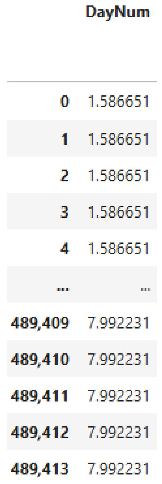
Figure 5. Sample of DayNum field from the VED dataset.

It is important to note that this aggregation results from dozens of files in the aforementioned CSV format, after decompression, and is subdivided into static data (metadata) and dynamic data.

For dynamic data, the files were used as shown in Table 5, Table 6 and Table 7. The original tabular configuration of this final file, for the vehicle with identifier “531”, can be evidenced with the most important columns marked in red (DayNum, VehId, Trip, Timestamp (ms), Latitude [deg] and Longitude [deg]).

Table 5. Vehicledata from the Vehicle Energy Dataset: Main identification fields.

DayNum 1	VehId 2	Trip 3	Timestamp (ms)	Latitude [deg]	Longitude [deg]
173.89	531	1091	0	42.26	−83.73
173.89	531	1091	100	42.26	−83.73
173.89	531	1091	700	42.26	−83.73
173.89	531	1091	800	42.26	−83.73
173.89	531	1091	1100	42.26	−83.73
7.78	531	629	0	46.01	42.24
7.78	531	629	100	46.01	42.24
7.78	531	629	200	46.01	42.24
7.78	531	629	300	46.52	42.24
7.78	531	629	400	46.01	42.24

¹ Crucial field for temporal ordering of trips; ² Vehicle identifier, crucial for distinguishing trips per vehicle; ³ Unique trip identifier, crucial for trip segmentation.

Table 6. Vehicle data from the Vehicle Energy Dataset: Performance metrics.

Speed [kph]	Engine RPM	Engine Load [%]	Absolute Power [kW]
17.0	132,400	17,342	13.73
30.0	132,400	17,342	13.73
39.0	132,400	9242	13.73
39.2	137,699	9242	13.73
46.0	217,899	9242	13.73
17.0	2.78	144.28	14.11
33.0	3.91	105.20	14.11
11.0	2.78	105.20	14.11
52.0	3.91	105.20	14.11
32.0	3.91	105.20	14.11

Table 7. Vehicle data from the Vehicle Energy Dataset: Energy parameters.

HV Battery SOC [%]	Fuel Consumption [%]
NaN	4.68
NaN	4.68
NaN	4.68
NaN	4.68

Longitude and latitude coordinates are in the Coordinate Reference System or EPSG (European Petroleum Survey Group), which serves as a unique identifier for the position and projection of a spatial feature in the geographic context (for example, “4326”, for decimal geographic coordinates, encompassing the entire planet, but centered on the specific locality of this research: Ann Arbor, Michigan, USA). It was necessary to convert them into a format with better readability for the computer, the Geometry, which is similar to WKT or Well-Known Text, but with its own configuration suitable for the GeoDataFrame data structure, representing binary data. The VehId field represents the vehicle identifier, while Trip represents the unique identifier of the trajectories.

Regarding the derivation of new fields, there was a need to address the temporal aspect. With the assistance of metadata for contextualized understanding of what each field represents, in addition to DayNum and Timestamp (ms), it was possible to design a “datetime” column derived from those two columns, serving both for processing trajectory segmentation and for derivation of the day field. Thus, the necessary data engineering essentially involved creating the datetime field, converting the Timestamp (ms) column to timestamps with the “D” parameter, indicating that this latter column represents “days”. Subsequently, based on reading the VED documentation, 1 November 2017 is determined as the beginning of the day count, based on the DayNum field. Following this, with the definition of the oldest and most recent timestamp, an interpolation is performed in which, in an initially empty dataframe called “t”, using the date_range method, a series of equally spaced dates (at the same interval) is created based on the size of the dataframe. Finally, the values of “t” are assigned to the new column of the first dataframe, with a conversion back to the datetime format and rounding of these data so that they are considered only up to seconds. In Table 8, the derived columns and data are presented, along with 2 columns, Day and Period.

Table 8. Vehicle trip data with derived temporal information.

VehId	Trip	Latitude [deg]	Longitude [deg]	Datetime	Day
560	2	42.252974	−83.674152	2017-11-02 12:05:45	Thursday
560	2	42.252974	−83.674152	2017-11-02 12:05:57	Thursday
560	2	42.252974	−83.674152	2017-11-02 12:06:08	Thursday
560	2	42.252974	−83.674152	2017-11-02 12:06:20	Thursday
560	2	42.252974	−83.674152	2017-11-02 12:06:32	Thursday
371	4411	42.282303	−83.734510	2018-11-11 11:35:46	Sunday
371	4411	42.282303	−83.734510	2018-11-11 11:35:58	Sunday
371	4411	42.282303	−83.734510	2018-11-11 11:36:10	Sunday
371	4411	42.282303	−83.734510	2018-11-11 11:36:22	Sunday
371	4411	42.282303	−83.734510	2018-11-11 11:36:34	Sunday

Notes: Datetime: Crucial for trajectory segmentation and temporal analysis; Day: Day of the week derived from Datetime, useful for contextualization.

In summary, through these initial tasks, it was possible to obtain the ordering based on the new Datetime field derived through data engineering and the derivation of the Day field, containing the days of the week. Figure 6 demonstrates the initial approach in the development process of the SSDF Method. This phase comprises raw data extraction, dataset concatenation, and the derivation of temporal attributes (DateTime and Day) necessary for subsequent trajectory analysis.

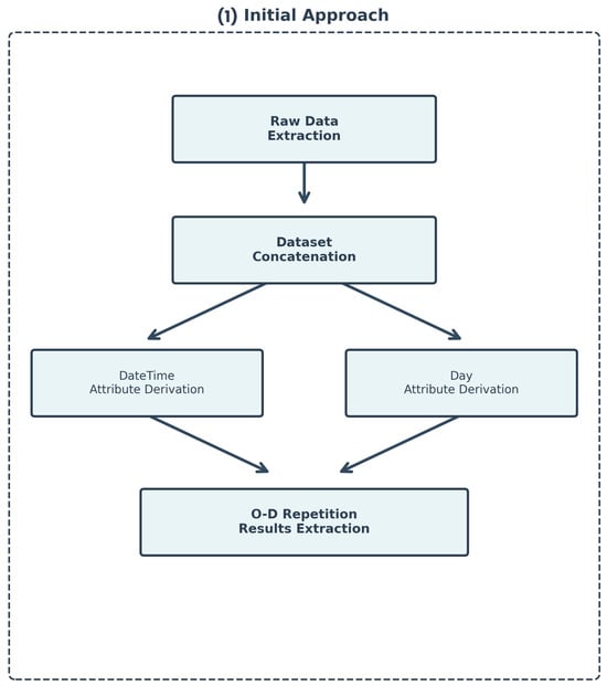
Figure 6. Initial approach flowchart for data processing.

However, it became necessary to segment these Trips, and subtrajectories were obtained based on this field. This need arose from the possibility of obtaining a better representation of the trips that an individual user would take. And it is this segmentation path that the next step addresses.

4.2. Segmentation

Following the approach proposed in [34], a stay-point based segmentation process was implemented using the MovingPandas library [55]. This procedure employs three parameters: 100 m as the maximum displacement threshold, 30 min as the minimum stopping time, and 1000 m to filter subtrajectories with at least this minimum length. Stay-point segmentation identifies periods when the vehicle remained stationary, enabling the partitioning of trajectories into meaningful segments suitable for modeling and analysis.

4.2.1. Parameter Selection and Justification

Trajectory segmentation parameters critically impact subtrajectory quality and subsequent destination prediction performance. Our parameter selection follows and adapts the methodological framework proposed by [34], who systematically evaluated stop detection parameters across multiple distance thresholds (10, 20, 50, 75, 100 m) and time thresholds (up to 15 min) for vehicle trajectory analysis.

Dataset Characteristics Influencing Parameter Selection:

• Vehicle Type: VED comprises exclusively private personal cars (individual passenger vehicles), which exhibit different stopping behavior compared to mixed traffic datasets containing commercial vehicles, buses, or taxis. Private cars tend to have longer dwelling times at destinations (e.g., home, workplace) and larger parking facility footprints compared to commercial fleet vehicles, motivating increased spatial tolerance.
• Driver Identity Ambiguity: Unlike datasets with explicit driver identification, VED cannot discriminate between different drivers of the same vehicle (e.g., family members, friends). Different drivers of the same car exhibit heterogeneous mobility patterns and stopping behaviors. Additionally, vehicles may remain stationary with occupants inside (idling, waiting) during intermediate stops, which would be incorrectly segmented with stricter time thresholds. This inherent heterogeneity necessitates more permissive temporal parameters.
• Mixed Urban-Highway Context: VED trajectories span diverse road hierarchies including highways, arterials, and local roads. Highway rest stops and service areas require larger spatial thresholds than purely urban datasets, as validated by [34] finding that threshold choice should reflect spatial context.
• GPS Precision Variability: One-year temporal coverage introduces seasonal variations in GPS accuracy (atmospheric conditions, satellite geometry). Increased spatial tolerance (100 m vs. 50 m) accommodates positioning uncertainty without sacrificing stop detection reliability.

Selected Parameters:

Following the framework proposed by [34] and considering VED-specific characteristics, we selected: distance threshold D = 100 m (=baseline), time threshold T = 30 min ($2\times$ baseline), and minimum trajectory length L = 1000 m.

• D = 100 m: Provides spatial tolerance for private car parking facilities (typically 50–100 m footprint for residential and commercial lots), GPS uncertainty, and mixed road contexts, while remaining within  [34] validated range (≤100 m). Values exceeding 100 m risk conflating distinct nearby destinations.
• T = 30 min: Accommodates idling periods, intermediate stops with occupants remaining in vehicle, and genuine dwelling periods characteristic of private car usage patterns. Preliminary testing with T = 15 min resulted in excessive trip fragmentation, particularly problematic given the heterogeneity of multiple drivers per vehicle. The 30 min threshold aligns with transportation planning definitions of “stop” (≥20–30 min) and filters transient pauses (e.g., traffic lights, brief errands) while capturing meaningful destination visits.
• L = 1000 m: Ensures subtrajectories contain sufficient spatial information for meaningful origin-destination analysis. Shorter trajectories (<1000 m) disproportionately represent parking lot maneuvers or GPS noise rather than genuine trips, degrading model training quality.

While more restrictive parameters following [34] baseline (50 m, 15 min) may be appropriate for homogeneous commercial fleet datasets with single-driver tracking, VED’s private car focus and multi-driver ambiguity justify the adapted parameters. Our selection prioritizes robustness across VED’s heterogeneous mobility patterns while remaining within validated parameter ranges from the literature.

4.2.2. Spatial Tessellation Grid Size

The tessellation grid cell size of 100 square meters (10 m × 10 m) was selected based on the spatial characteristics of the Ann Arbor urban area and the resolution requirements for meaningful Origin–Destination analysis. This granularity provides:

• Urban Scale Appropriateness: Ann Arbor’s street block sizes typically range from 100–200 m, making 10 m cells suitable for distinguishing individual destinations (parking lots, building entrances) while avoiding excessive fragmentation. This scale captures the natural spatial structure of urban mobility decision points.
• GPS Accuracy Alignment: Consumer-grade GPS devices (used in VED) typically achieve 5–10 m accuracy under good conditions. The 100 m² cells provide a 2:1 safety margin, reducing spurious state transitions from GPS jitter while maintaining spatial precision for destination differentiation.
• Computational Efficiency: Finer tessellations (e.g., 25 m²) would quadruple the state space size, increasing transition matrix sparsity and computational requirements without proportional gains in prediction accuracy for vehicle-scale movements. The selected granularity balances model complexity and predictive power.
• Semantic Meaningfulness: 100 m² cells approximate typical parking facility footprints and building lots, aligning with natural mobility decision units rather than arbitrary subdivisions. This semantic coherence ensures that spatial states correspond to meaningful locations in the urban environment.

This tessellation scale balances spatial resolution, computational tractability, and GPS uncertainty while capturing the essential spatial structure of vehicle mobility patterns in the study region. Alternative grid sizes (e.g., 25 m², 400 m²) were considered but rejected, due to either excessive computational burden or insufficient spatial precision for destination discrimination.

4.2.3. Segmentation Workflow

When segmenting trajectories, subtrajectories emerge. For this research, these consist of partitioning trajectories by abstracting moments in which the trajectory is recorded as points without movement (time passes, but there is permanence within a delimited region for 30 min). For example, trajectory 132 becomes 132.1, 132.2, and 132.3, based on the separation between the moments seen in 132.1 until a moment when temporal continuity is lost, and then returns to the beginning of 132.2. The same logic follows for 132.3 and as many other subtrajectories as exist until the end of the parent segment 132, as long as it is at least 1000 m long.

The sequence of tasks for this step proceeds as follows: First, trajectories are obtained using MovingPandas, described in [56], from the original dataset, and these trajectories are subsequently used to derive subtrajectories. Subsequently, the Origin (O) and Destination (D) points are extracted from these subtrajectories. Through tessellation applied to 100-square-meter grids, the Origin and Destination points are then aggregated with their corresponding grid labels, incorporating the day column. Finally, the labels for the origin and destination cells are merged to produce the final output, which constitutes the result of this integration process.

Figure 7 presents the trajectory segmentation workflow, which transforms complete vehicle trajectories into analyzable Origin–Destination pairs. The process initiates with trajectory data acquisition and proceeds to subtrajectory extraction, dividing continuous paths into discrete segments. These subtrajectories maintain the same format as the source trajectories, necessitating the extraction of origin and destination cells in conjunction with the tessellation process. The workflow then branches into parallel extraction of origin and destination points, which are subsequently mapped to a spatial tessellation grid. This tessellation is conducted using the region depicted in Figure 8 as the defining parameter, encompassing the city of Ann Arbor and four adjacent districts. The tessellation mapping converts geographic coordinates into discrete spatial states, enabling the application of Markovian models. Finally, temporal attributes are integrated, and O-D pairs are aggregated to form the structured dataset required for prediction modeling.

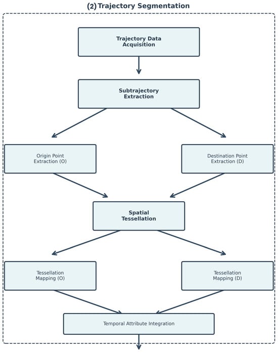
Figure 7. Trajectory segmentation workflow for O-D pair extraction and aggregation.

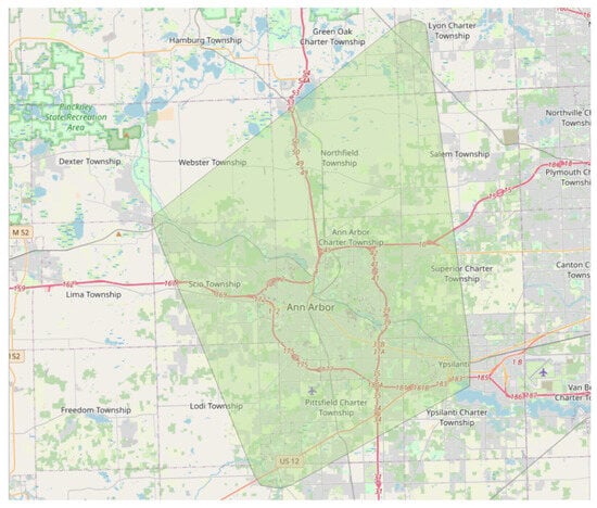
Figure 8. Spatial tessellation boundaries for the study region encompassing Ann Arbor and four adjacent districts.

The tessellation grid defines the discrete spatial states used for Markovian modeling, dividing the geographic area into regular cells that serve as the fundamental units for Origin–Destination pair identification. This spatial discretization enables the conversion of continuous GPS coordinates into categorical location states required for probability transition matrix construction. Finally, at the end of this phase, the Consolidation process integrates these spatial mappings with frequency computations, as described in the following section.

4.3. Consolidation

Figure 9 illustrates the consolidation phase, where processed O-D pairs are transformed into frequency distributions suitable for statistical modeling. This stage involved a data integrity validation procedure consisting of systematic repetitions to ensure correct application of the MovingPandas library method for subtrajectory generation. The workflow computes the frequency of each unique Origin–Destination pair derived from subtrajectories rather than complete trajectories, capturing the repetition patterns that characterize vehicular movement behavior. The frequency computation algorithm processes the segmented trajectory data and generates occurrence counts for each O-D pair. Subsequently, the frequency table integration step merges these computations with the spatial tessellation mapping (junction of Origin and Destination grid labels), producing a unified data structure that provides the empirical probability distributions required for both Markov Chain and Hidden Markov Model training. This consolidation ensures that the models are built upon statistically representative patterns extracted from discrete trajectory segments rather than entire trip sequences.

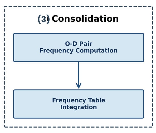
Figure 9. Consolidation phase for O-D pair frequency aggregation.

The Consolidation phase integrates outputs from both the General Exploration and the Preparation stages. The frequency counting algorithm processes the Origin–Destination pairs. It generates occurrence statistics for each unique O-D combination. This frequency table is then merged with the prepared dataset, combining spatial tessellation mapping with temporal repetition patterns.

The sample filtering process employed a matrix-based criterion. Cells represent vehicles exhibiting different levels of trajectory repetition. Vehicles were categorized by the number of trajectories with recurring O-D patterns. Categories ranged from 2 or more repeated trajectories with 2 or more repetitions, incrementally up to 6 or more repeated trajectories with 6 or more repetitions. Initially, 99 vehicles met the most stringent criterion (6+ trajectories with 6+ repetitions).

The automatic threshold selection algorithm (Algorithm 1) further refined this sample. It evaluated statistical adequacy for both Markov Chain and Hidden Markov Model requirements by testing candidate values from the set {10, 15, 20, 25, 30, 35, 40, 50} trajectory sequences per vehicle. The algorithm determined an optimal threshold of 50 trajectory sequences per vehicle. This threshold was selected because, without filtering, Markov Chains and HMMs performed optimally on different vehicle subsets, preventing proper vehicle pairing for statistical validation (e.g., paired t-tests). Additionally, lower thresholds yielded reduced mean precision values, while the threshold of 50 minimized prediction failures during cross-validation folds, a critical issue for HMM inference. Conversely, higher thresholds would further constrain the dataset, reducing the vehicle sample size and consequently limiting representativeness. This balanced model reliability with data retention and maintained consistency with the theoretical probability frameworks. Applying this threshold to the 99-vehicle subset yielded a final sample of 23 vehicles, reducing the number of records from 3776 to 2129. Each possessed sufficient trajectory data to support robust statistical inference while maintaining representative behavioral patterns. With this filtered dataset of 23 vehicles, the second research phase commenced. It consisted of statistical analysis, prediction modeling, and comparative evaluation. However, additional data preparation steps were required before model training and validation.

A necessary observation is that one vehicle from the original 99-vehicle dataset was excluded during the origin–destination pair consolidation phase. This vehicle exhibited exclusively unique trajectories, with no recurring origin–destination patterns across the entire collection period. Since probabilistic modeling requires trajectory recurrence to estimate transition probabilities from observed frequency distributions, this vehicle could not be incorporated into the analysis. Consequently, the working dataset comprised 98 vehicles, which were subsequently processed through the SSDF filtering method, ultimately yielding the final sample of 23 vehicles used in the experiments.

4.4. Final Dataset Generation with Data Balancing

For modeling with Markov Chains and HMM and subsequent prediction execution, filtering was performed through data balancing to mitigate issues related to insufficient data for statistical validation or scenarios in which the algorithms lack the minimum processing elements. From these considerations, it was observed that there was a need to balance the data to improve precision. After processing and visualizing the sample data, the distribution of repetitions before balancing is shown in Figure 10.

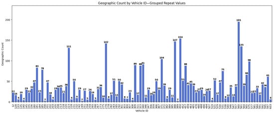
Figure 10. Bar chart with the distribution of repetitions before data balancing.

As previously described, the automatic threshold selection algorithm (Algorithm 1) determined an optimal threshold of 50 trajectory sequences per vehicle, yielding a final sample of 23 vehicles with 2129 records from the original 98-vehicle subset.

This threshold was determined through systematic evaluation of predefined values $[10,15,20,25,30,35,40,50]$ using a combined scoring function that assesses statistical adequacy for both Markov Chains and HMMs simultaneously. The selection was based exclusively on mathematical criteria of statistical fitness conducted prior to any model training, not on observed prediction performance, ensuring vehicle selection independence from subsequent model outcomes.

Thresholds below 50 demonstrated insufficient statistical adequacy according to the scoring function, while higher values would excessively constrain the dataset, reducing vehicle sample size and consequently limiting representativeness. The selected threshold thus balances statistical rigor with dataset adequacy, maintaining consistency with the theoretical framework established in the  Section 3. Figure 11 displays the resulting distribution of trajectory repetitions after balancing (bars show counts ≥50; lower values excluded).

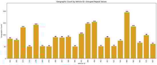
Figure 11. Bar chart with the distribution of repetitions after data balancing.

The following section describes the implementation of the prediction models based on Markov Chains and Hidden Markov Models.

The algorithm determines the optimal trajectory sequence threshold by evaluating multiple candidate values against two criteria: Markov Chain statistical adequacy ($adequac{y}_{MC}$) and Hidden Markov Model parameter sufficiency ($adequac{y}_{HMM}$). The combined score balances model reliability with data retention, penalizing excessive filtering through the $facto{r}_{retention}$ term. The threshold maximizing this composite metric ($scor{e}_{final}$) is selected for final data preparation.

The adequacy criteria in Algorithm 1 are grounded in statistical requirements for probabilistic models. Anderson and Goodman [50] derived asymptotic properties of transition probability estimators in Markov Chains, providing the theoretical foundation for assessing estimation quality. Rabiner [45] established that HMMs require sufficient training data relative to model complexity, specifically the number of parameters (N² transition probabilities plus N × M emission probabilities) must be adequately supported by available observations to avoid overfitting. Additionally, Froehlich and Krumm [57] empirically demonstrated that trajectory repetitions improve destination prediction accuracy, observing that “predictions for repeated trips are generally more accurate than those for all trips” in a dataset comprising 14,468 trips from 252 drivers, and that “longer observation times result in the discovery of more driver repetition, meaning that prediction accuracy rises as the driver is observed for more days.” The requirement for multiple trajectory repetitions is thus not an arbitrary assumption, but an established finding in the mobility prediction literature.

4.5. Implementation

Following the preprocessing pipeline described in Section 4.1, Section 4.2, Section 4.3 and Section 4.4, which produces the final trajectory dataset, two prediction models were implemented: a Markov Chain-based predictor and a Hidden Markov Model-based predictor. This section details the architectural design and implementation specifics of both approaches. Section 4.5.1 describes the Markov Chain predictor, Section 4.5.2 presents the HMM predictor, and Section 4.5.3 outlines the training and testing procedures employed for model evaluation.

4.5.1. Markov Chains Predictor

Algorithm 2 presents the function that constructs the transition matrix for the Markov Chains predictor, incorporating Laplace smoothing to handle sparse data.

Algorithm 2 Markov Chains Transition Matrix Creation

1: function createDisplacementsTransitionMatrix(dataset, vehId, $\alpha$)   2:     Initialize transitionCounts with smoothing   3:                     ▹ Count origin-to-destination transitions   4:     for $i=0$ to $\left|dataset\right|-1$ do   5:         $s_{origin}\leftarrow$ dataset[i].origin   6:         $s_{dest}\leftarrow$ dataset[i].destination   7:         transitionCounts[$s_{origin}$][$s_{dest}$] ← transitionCounts[$s_{origin}$][$s_{dest}$] + 1   8:     end for   9:     $P\leftarrow$ normalizeRows(transitionCounts) 10:      return P 11: end function

Algorithm 2 constructs the transition probability matrix by counting origin-to-destination transitions in the training data. The matrix is initialized with Laplace smoothing parameter $\alpha$ to prevent zero probabilities for unobserved transitions (line 2). For each trajectory record, the algorithm counts the transition from origin grid $s_{origin}$ to destination grid $s_{dest}$ (lines 4–7). After counting all transitions, row normalization produces the probability matrix P where $P\left[i\right]\left[j\right]$ represents the probability of transitioning from origin state i to destination state j (line 9). During prediction, given a test trajectory with known origin grid $s_{origin}$, the model selects the destination with maximum transition probability: ${\widehat{s}}_{dest}=arg{max}_{j}P\left[s_{origin}\right]\left[j\right]$.

4.5.2. HMM Predictor

The HMM predictor extends the Markov Chains approach by incorporating emission probabilities to model the relationship between contextual information and destination patterns. In this formulation, destination grid cells constitute the state space (representing the prediction target), while composite observations formed by pairing day of week with origin grid cells serve as the observable symbols (e.g., ⟨Monday, grid_150⟩). The emission probability matrix encodes $P(\mathrm{observation}\mid \mathrm{destination})$, enabling the model to learn how specific origin–day contexts relate to destination outcomes. During prediction, given an observed context (origin and day), the model infers the most probable destination state. This architectural design differs from sequential HMM applications where observations form temporal sequences: here, each trajectory is treated as an independent prediction task with a single contextual observation, rather than a time-varying sequence of sensor measurements.

Algorithm 3 constructs the HMM probability matrices by counting co-occurrences in the training data. The transition matrix A captures sequential patterns between destination states (lines 3–7), while the emission matrix B encodes the conditional relationship between destinations and composite observations formed by pairing day of week with origin grid (lines 9–13). During prediction, given a test trajectory with known origin grid $g_{\mathrm{origin}}$ and day of week d, the composite observation symbol $o=⟨d,g_{\mathrm{origin}}⟩$ is constructed. The Viterbi algorithm then computes the most probable destination state by maximizing: ${\widehat{s}}_{\mathrm{dest}}=arg{max}_{s}P(s\mid o)\propto P(o\mid s)·P\left(s\right)$, where $P(o\mid s)$ is retrieved from the emission matrix B and $P\left(s\right)$ from the initial state distribution. Unlike sequential HMM applications that decode temporal observation sequences, this formulation performs direct probabilistic inference conditioned on a single contextual observation.

Algorithm 3 Creation of HMM Matrices

1: function createHMMMatrices(dataset, vehId)   2:     Initialize transitionCounts, emissionCounts with smoothing   3:                  ▹ Count destination-to-destination transitions   4:     for $i=0$ to $\left|dataset\right|-2$ do   5:          $s_{current}\leftarrow$ dataset[i].destination   6:          $s_{next}\leftarrow$ dataset[$i+1$].destination   7:          transitionCounts[$s_{current}$][$s_{next}$] ← transitionCounts[$s_{current}$][$s_{next}$] + 1   8:     end for   9:                  ▹ Count emissions: destination ← (day, origin) 10:      for $i=0$ to $\left|dataset\right|-1$ do 11:           $s\leftarrow$ dataset[i].destination 12:           $o\leftarrow ⟨$ dataset[i].day, dataset[i].origin⟩ 13:           emissionCounts[s][o] ← emissionCounts[s][o] + 1 14:      end for 15:       $A\leftarrow$ normalizeRows(transitionCounts) 16:       $B\leftarrow$ normalizeRows(emissionCounts) 17:       return A, B 18: end function

4.5.3. Training and Testing Stages

The training and testing procedures employ K-fold cross-validation (K = 10) with shuffling to evaluate model performance. For each of the 23 vehicles, the displacement dataset was partitioned into 10 mutually exclusive folds. In each iteration, the K-Fold algorithm generates two disjoint index sets: train_index (containing 9 folds) and test_index (containing 1 fold), ensuring complete separation between training and testing data.

The training phase exclusively uses the data indexed by train_index to construct the model parameters. For the Markov Chains model, Algorithm 2 (createDisplacementsTransitionMatrix) processes only the training subset (vehicle_train) to construct the transition probability matrix. For the HMM model, Algorithm 3 (createHMMMatrices) similarly constructs both the transition matrix and the emission probability matrix using only the training subset. The implementation initially configured unique states corresponding to the labels of origin and destination grids where vehicle movement occurred.

The testing phase exclusively uses the data indexed by test_index (vehicle_test), which contains no samples from the training set. Predictions were generated on this held-out test subset using the Viterbi algorithm for HMM and maximum likelihood state transitions for Markov Chains. Precision was computed by comparing predictions against the true destinations in the test subset.

This process was repeated across all 10 folds, with each fold serving as the test set exactly once while the remaining nine folds formed the training set. The strict separation between train_index and test_index in each iteration eliminates any possibility of data leakage, yielding 10 independent precision measurements per vehicle for subsequent statistical analysis. The 10-fold cross-validation framework ensures that model evaluation reflects genuine predictive performance on unseen data.

The term “independent precision measurements”, mentioned above, refers to the statistical independence of train/test partitions within each fold of the K-fold cross-validation, not to the absence of recurring spatial patterns. Each fold partitions the trajectory set such that training and testing subsets are temporally disjoint (without instance overlap). The 10 repetitions employ different random seeds, generating distinct partitionings that produce 100 precision estimates per vehicle (10 folds × 10 repetitions). Although origin–destination pairs may recur geographically, which is expected in human mobility patterns, each trajectory possesses a unique timestamp, representing distinct temporal events.

Regarding the use of HMMs, the approach is oriented toward human movement patterns, particularly when enhanced by the model’s requirement for not only the transition matrix and unique training states, but also the emission matrix and symbols to be combined with the hidden states. Specifically, the symbols emerge from the consideration of each day of the week combined with the origin grid, thus corresponding to the departures of each vehicle, and are integrated with the emission matrix (which, unlike the transition matrix, need not be square). A simple example can be considered using the emission: ⟨Monday, 150⟩, where Monday represents the day of initiation of a movement, and 150 represents the label of a hypothetical origin grid.

The emission matrix structure enables context-aware prediction by encoding the relationship between hidden states and observable temporal-spatial combinations. This framework captures systematic variations in movement behavior across different days of the week, recognizing that destination preferences may exhibit cyclical patterns tied to weekly routines. By integrating both transition probabilities and emission probabilities, the HMM leverages complementary sources of information, spatial movement sequences and temporal context, to enhance predictive accuracy beyond what standard Markov Chains can achieve.

4.6. Language Assistance

The manuscript was originally written in Portuguese and translated to English using Claude AI, version Sonnet 4.5 (Anthropic, San Francisco, CA, USA, 2025). The AI tool was used exclusively for language translation and stylistic improvement to enhance readability for an international audience. All research design, methodology, data collection, analysis, and interpretation were conducted independently by the authors without AI involvement.

5. Experiments

The experimental evaluation employed real-world vehicle trajectory data from the Vehicle Energy Dataset (VED) [53]. The VED provides comprehensive GPS trajectories that can be processed for destination prediction tasks. For this research, trajectories were extracted using the geographical coordinates, trip identifier, and timestamp (in microseconds) columns from the dataset.

The data were collected in agreement between the University of Michigan and the Idaho National Laboratory. This was done with the objective of studying user behavior regarding energy consumption and the potential savings of eco-driving technologies.

The same authors evidence that there are 383 vehicles (actually 384, according to the correction made in github) in routes traveled between the period of 1 November 2017 and 9 November 2018, in Ann Arbor (city south of Michigan). The vehicles are of different types, but in this work these types are not relevant. Basically, they vary from passenger vehicles (common cars) to light trucks. The total distance traveled, during 1 year and 8 days was 373,964 miles.

With the metadata formed by a table (static data with vehicle type, vehicle class, engine configuration, engine displacement, transmission, wheels and weight) and the dataset in “csv” format, a de-identification process was performed for the researchers’ work, which consisted of: Random Fogging, Geofencing and Major Intersections Bounding, according to [54].

Regarding the data, there were still some difficulties: initially, mainly due to the way of reading the timestamp, which defined the beginning of the experiments’ course, with the prior treatment of the data through the derivation of the datetime column.

This dataset has two types of tabular files: dynamic data and static data. The static data can be seen as metadata. They contain, according to [54], the vehicle type (in general, whether it is electric, hybrid or conventional), the vehicle class (common car, SUV or light truck), engine configuration, engine displacement, transmission, wheels and weight.

The data used in this research have, by choice, 99 of the vehicles from the 6+ by 6+ cell as seen in the matrix already presented in Section 4; however, only 23 of these were effectively used in the sampling. The reason for this filtering is due both to the decrease in processing complexity, from 384 to 99 vehicles, and mainly due to the consideration of sub-trajectories and those vehicles with the highest number of routes—these having the highest number of repetitions, allowing for an improvement in precision performance based on the assumption that more repetitions leads to better performance due to the existence of more historical data for predictions.

The initial trajectory segmentation process generated varying numbers of origin–destination pairs for each vehicle in the dataset, reflecting natural differences in mobility patterns, data collection periods, and vehicle usage intensity. Table 9 presents the complete distribution of trajectory counts across all 98 vehicles before applying any sample size threshold. This raw distribution reveals substantial heterogeneity: trajectory counts range from as few as 2 (vehicles 200 and 389) to as many as 195 (vehicle 560), with a median of 29 trajectories per vehicle. Such variability presents methodological challenges for comparative statistical analysis and model training, as vehicles with very few trajectories may not provide sufficient data for reliable transition probability estimation in Markov models.

Table 9. Geographic Count by Vehicle ID: Grouped Repeat Values.

Vehicle	Count	Vehicle	Count	Vehicle	Count
12	22	273	36	459	41
128	16	275	10	463	45
133	6	276	142	465	39
135	19	278	8	476	23
140	4	282	17	480	27
145	29	283	51	488	29
155	22	285	13	490	14
156	32	292	50	494	26
180	47	301	42	507	27
181	83	303	8	519	4
184	23	304	7	521	52
185	78	307	23	529	17
200	2	308	4	530	47
201	47	309	89	531	75
202	18	311	17	538	8
203	6	323	88	540	12
205	29	340	91	546	35
208	34	346	11	547	13
213	35	347	29	557	37
218	21	356	16	560	195
220	38	359	19	561	135
223	131	366	50	564	39
228	6	367	29	565	66
231	50	371	104	575	98
232	9	372	39	577	21
242	29	382	8	581	22
249	2	384	29	584	33
251	27	385	11	591	17
258	5	388	147	592	42
259	26	389	2	595	36
265	19	450	154	597	61
266	5	452	51	603	6
267	31	457	88	—	—

The heterogeneity observed in Table 9 reflects both systematic and stochastic factors in GPS trajectory collection. Systematic factors include variations in monitoring periods, as some vehicles may have been tracked for longer durations, and differences in vehicle operational patterns, where commercial or frequently-used vehicles naturally generate more trajectories than occasionally used personal vehicles. Stochastic factors encompass GPS signal interruptions, data transmission failures, and environmental conditions affecting location accuracy. Vehicles with very low trajectory counts (fewer than 10 trajectories) are particularly problematic for probabilistic modeling: sparse data yields unreliable transition matrix estimates characterized by high variance and potential overfitting to idiosyncratic movement patterns. This sparsity issue becomes critical when estimating transition probabilities between specific origin–destination pairs, where insufficient observations can result in zero-probability estimates for valid transitions or artificially inflated probabilities for rarely-observed patterns. The distribution further indicates that approximately 60% of vehicles fall below the 50-trajectory threshold, motivating the need for systematic sample size filtering to ensure model reliability.

To ensure statistical reliability and model generalizability, we implemented a minimum threshold of 50 trajectories per vehicle, following established practices in the trajectory mining and Markov-based prediction literature. This threshold value represents a carefully considered balance between competing methodological requirements: it must be sufficiently large to enable stable transition probability estimation with acceptable confidence intervals, yet not so restrictive as to eliminate most vehicles from analysis. Table 10 presents the filtered dataset comprising 23 vehicles that satisfied this criterion, collectively generating 2083 origin–destination pairs. The filtering process reduced the vehicle sample from 98 to 23 (a 76.5% reduction in vehicle count), but retained approximately 41% of the total trajectory data, indicating that the excluded vehicles were predominantly those with sparse mobility records. This trade-off prioritizes model quality over sample quantity: working with adequately-sampled vehicles enables more robust cross-validation, reduces estimation variance, and facilitates meaningful inter-vehicle performance comparisons without confounding effects from data scarcity.

Table 10. Geo Count by Vehicle ID: Grouped Repeat Values (After Filtering).

Vehicle	Count
181	83
185	78
223	131
231	50
276	142
283	51
292	50
309	89
323	88
340	91
366	50
371	104
388	147
450	154
452	51
457	88
521	52
531	75
560	195
561	135
565	66
575	98
597	61

The filtered dataset in Table 10 exhibits substantially improved characteristics for statistical modeling compared to the original distribution. Trajectory counts now range from 50 to 195, with a mean of 90.6 trajectories per vehicle and a standard deviation of 40.8, representing a more homogeneous distribution that reduces inter-vehicle variance in parameter estimation quality. This homogeneity is methodologically important because it ensures that performance differences between vehicles reflect genuine variability in mobility patterns rather than artifacts of sample size disparities. The 50-trajectory threshold provides sufficient data for reliable 10-fold cross-validation: with an average of 90 trajectories per vehicle, each training fold contains approximately 81 trajectories, enabling robust transition matrix estimation even for vehicles with complex movement patterns involving numerous origin–destination pairs. Furthermore, this sample size adequately supports fair comparison between Markov Chains and Hidden Markov Models, as the more parameter-intensive HMM approach requires sufficient data to estimate both transition and emission matrices without overfitting. It is important to emphasize that only spatial trajectory repetitions (unique origin–destination pairs) were considered in this count, not temporal repetitions, each counted trajectory represents a distinct spatial movement pattern regardless of occurrence frequency over time, ensuring that our models learn spatial transition structures rather than temporal periodicities.

We sought to act on an elaborately prepared dataset in an equivalent manner. For both cases, only geographical repetitions were considered, and not temporal ones.

In the next section, a description of the experimental plan is given.

5.1. Experimental Planning

Figure 12 presents the evaluation workflow executed for the 23 vehicles using 10-fold cross-validation. For the HMM implementation, the Viterbi algorithm was employed. Since only this model generated normalized results in this evaluation context, the paired t-test was applied for statistical comparison, following the guidelines established by [58].

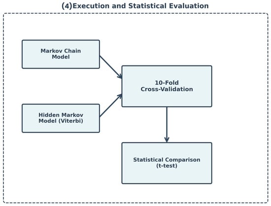
Figure 12. Execution and statistical evaluation workflow comparing Markov Chain and Hidden Markov Model performance using 10-fold cross-validation.

At the end, the method allows for evaluation with t-student, leading to a final framework capable of interpretation and validation, containing pairs with statistical significance and pairs without statistical significance. Another factor is the Research Question and the Hypothesis that there is a significantly relevant difference between the techniques. The Research Question in this context is: “Is there a difference regarding the use of destination prediction models based on Markov Chains and HMM, in the context of urban traffic and use of individual vehicles, with relation to a metric such as precision?”. Thus, the test was configured to determine if H0 = There is no difference or H1 = There is a difference.

Regarding the choice of Precision (instead of, for example, Accuracy), it was due to the research question, considering the Precision formula in which true positives are divided by the sum of true positives with false positives. In this case, reproducibility is considered, the consistency of values, and not necessarily the proximity to a true value.

5.2. Achieved Results

Following the statistical validation procedure, the Shapiro–Wilk test was first conducted, confirming the normality of both sets of mean precisions for Markov chains and HMMs. Subsequently, paired Student’s t-tests were applied to the results when data structure allowed, adapting to unpaired tests when necessary.

Statistical Testing Methodology: The p-values reported in this study were calculated based on paired comparisons at the fold level within the 10-fold cross-validation framework. For each vehicle, we obtained 10 precision measurements (one per fold) for both the Markov Chain and HMM approaches. The paired t-test compares these 10 paired observations per vehicle, testing the null hypothesis that the mean difference between the two models equals zero. For the global analysis across all vehicles, we aggregated the fold-level results to compute vehicle-level mean precisions, then applied paired tests across the 23 vehicles. This approach enables interpretation based primarily on the graphs derived from the experimental outcomes while maintaining statistical rigor at both the vehicle and global levels.

Geographic repetition (the same origin–destination pair traversed multiple times) constitutes precisely the phenomenon that the models aim to capture, not a methodological confounder. Froehlich and Krumm [57] observed that “nearly 60% of trips were duplicated” in drivers monitored for 40+ days, and their prediction models explicitly learn origin–destination pair frequencies from historical patterns. Each instance of a route (e.g., home → work on Monday vs. home → work on Wednesday) possesses unique temporal context, distinct traffic conditions, and individualized decision circumstances. The K-fold structure ensures that these temporal instances are separated between training and testing sets, preserving statistical validity.

For statistical analysis, we applied independent samples t-tests (ttest_ind) comparing precision distributions between Markov Chains and HMMs. Although folds are paired by vehicle (same vehicle, same repetition, same fold), we used independent samples tests because we compare two distinct precision distributions (one from Markov, another from HMM) obtained under identical experimental conditions. The final unit of analysis consists of vehicle-level means (calculated from 100 folds each), which are then compared between the two models. This hierarchical structure (folds within vehicles, vehicles as comparison units) is appropriate for repeated cross-validation with independent sample t-tests.

5.2.1. Precision-Based Evaluation

The global precision averages are shown in Figure 13. Globally, considering the 23 vehicles, the HMM achieved a mean precision of 0.6101 compared to 0.5908 for the Markov Chain model, with a statistically significant p-value of 0.0248.

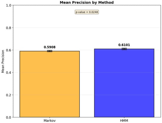
Figure 13. Global mean precision for Markov chains and HMMs across all vehicles.

Detailed results at the vehicle level are presented in Figure 14. The left panel displays the average precision per vehicle, with bars divided between Markov chains (blue) and HMMs (orange). The right panel shows p-values per vehicle on a logarithmic scale, with statistically significant values (p < 0.05) highlighted in orange. The dashed line indicates the threshold between significant and non-significant differences. Each vehicle-level p-value was computed from the paired t-test on the 10 fold-level precision values for that specific vehicle.

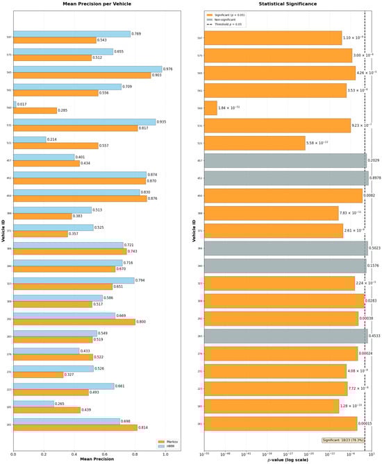
Figure 14. Paired analysis of precision: mean precision values per vehicle (left) and statistical significance of differences (right). Significant differences are observed in 18 out of 23 vehicles (78.3%).

Table 11 presents the comparative prediction performance between Markov Chain (MC) and Hidden Markov Model (HMM) approaches across the 23 filtered vehicles, evaluated using mean precision values from 10-fold cross-validation. Precision measures the proportion of correctly predicted destinations among all predictions made by each model, providing insight into prediction accuracy when the model commits to a specific destination forecast. The p-values reported in the rightmost column derive from paired t-tests comparing the precision distributions across the 10 validation folds for each vehicle, testing the null hypothesis that both models achieve equivalent performance. Values marked with asterisks indicate statistically significant differences at the conventional $\alpha =0.05$ threshold, while unmarked values suggest that observed performance differences could reasonably arise from random variation alone.

Table 11. Mean precision values and statistical significance for Markov Chain and Hidden Markov Model predictions across vehicles.

Vehicle ID	Markov Chain	HMM	p-Value
181	0.8144	0.6985	${10}^{-4}$ *
185	0.4393	0.2652	${10}^{-10}$ *
223	0.4934	0.6608	${10}^{-8}$ *
231	0.3267	0.5261	${10}^{-8}$ *
276	0.5222	0.4326	${10}^{-4}$ *
283	0.5190	0.5490	0.450
292	0.8003	0.6687	${10}^{-4}$ *
309	0.5175	0.5856	0.028 *
323	0.6508	0.7938	${10}^{-5}$ *
340	0.6697	0.7187	0.136
366	0.7434	0.7210	0.505
371	0.3568	0.5246	${10}^{-9}$ *
388	0.3826	0.5126	${10}^{-11}$ *
450	0.8761	0.8298	0.008 *
452	0.8698	0.8742	0.898
457	0.4342	0.4005	0.203
521	0.5566	0.2136	${10}^{-22}$ *
531	0.8165	0.9346	${10}^{-7}$ *
560	0.2850	0.0172	${10}^{-51}$ *
561	0.5563	0.7111	${10}^{-8}$ *
565	0.9034	0.9762	${10}^{-5}$ *
575	0.5123	0.6546	${10}^{-6}$ *
597	0.5431	0.7690	${10}^{-9}$ *

Values shown as ${10}^x$ represent p-values in scientific notation. * Indicates statistical significance at $p<0.05$. Global p-value = 0.0248. 18 out of 23 vehicles (78.3%) showed significant differences.

The results reveal substantial inter-vehicle heterogeneity in model performance and superiority patterns. Among the 23 vehicles analyzed, 18 (78.3%) exhibited statistically significant performance differences between the two approaches, indicating that model selection genuinely affects prediction quality for the majority of cases. Notably, the direction of superiority varies across vehicles: HMM outperforms MC in 13 vehicles (e.g., vehicle 531: HMM = 0.9346 vs. MC = 0.8165), while MC demonstrates superior performance in 5 vehicles (e.g., vehicle 560: MC = 0.2850 vs. HMM = 0.0172). For the remaining 5 vehicles (283, 340, 366, 452, 457), performance differences lack statistical significance, suggesting equivalent predictive capability. This heterogeneity underscores the importance of considering individual mobility pattern characteristics when selecting prediction models, as no single approach universally dominates across all trajectory profiles. The global p-value of 0.0248 from aggregate analysis indicates that, when considering the entire vehicle population, the observed performance differences between models are statistically significant and not attributable to chance alone.

5.2.2. Multi-Metric Evaluation and Performance Trade-Offs

To provide a more comprehensive assessment of model performance and address potential limitations of single-metric evaluation, we extended the analysis to include recall and F1-score alongside precision. Figure 15 presents the statistical comparison across all three metrics using paired t-tests, calculated using the same fold-level paired comparison methodology described above.

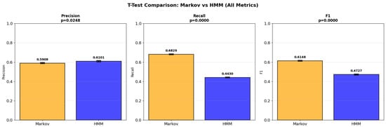
Figure 15. Paired t-test comparison of Markov chains and HMMs across three evaluation metrics: precision, recall, and F1-score. All differences are statistically significant (p < 0.05).

While the HMM demonstrated marginally superior precision (0.6101 vs. 0.5908, p = 0.0248), the Markov Chain model significantly outperformed the HMM in both recall (0.6829 vs. 0.4430, p < 0.0001) and F1-score (0.6148 vs. 0.4727, p < 0.0001).

Figure 16 and Figure 17 present the detailed paired analysis for recall and F1-score, respectively, following the same structure as the precision analysis. For recall, 22 out of 23 vehicles (95.7%) showed statistically significant differences, while for F1-score, 20 out of 23 vehicles (87.0%) exhibited significant differences.

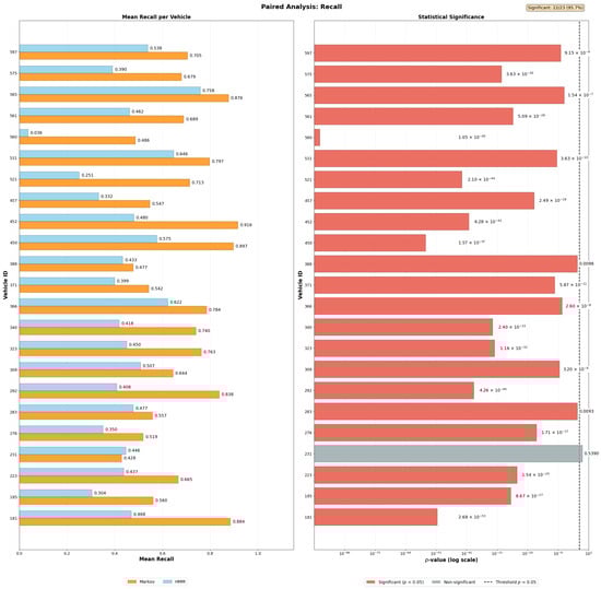
Figure 16. Paired analysis of recall: mean recall values per vehicle (left) and statistical significance of differences (right). Significant differences are observed in 22 out of 23 vehicles (95.7%).

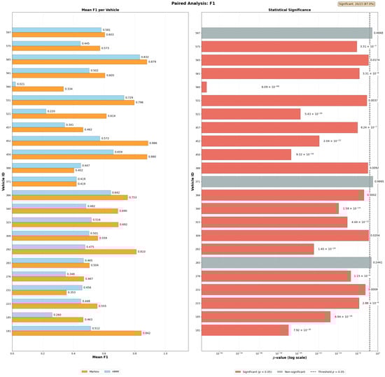
Figure 17. Paired analysis of F1-score: mean F1 values per vehicle (left) and statistical significance of differences (right). Significant differences are observed in 20 out of 23 vehicles (87.0%).

The cases where Markov chains achieved superior recall and F1-score compared to HMMs are due to inherent limitations in the HMM architecture regarding the day of the week and origin grid (origin grid tag), which filter the results making the probabilities more restricted. For example, if previously there would be X possibilities across the 7 days of the week, now there are Y possibilities for Wednesdays, where Y equals X minus the other 6 days of the week. This filtering effect constrains the HMM’s prediction coverage, resulting in lower recall despite higher precision.

5.2.3. Performance Distribution Analysis

To further illustrate the performance differences between the two approaches, Figure 18 presents scatter plots comparing Markov Chain and HMM performance across all three metrics for each vehicle. Points above the diagonal line indicate superior HMM performance, while points below indicate superior Markov Chain performance. The Pearson correlation coefficients (r) between the two models are 0.700 for precision, 0.501 for recall, and 0.710 for F1-score, suggesting moderate to strong agreement in relative vehicle-level performance rankings despite systematic differences in absolute values.

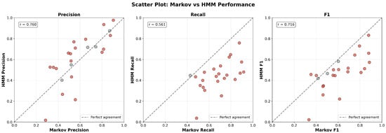
Figure 18. Scatter plot comparison of Markov Chain versus HMM performance across precision, recall, and F1-score. Red points indicate statistically significant differences (p < 0.05), while gray points indicate non-significant differences. The dashed line represents perfect agreement between models.

Figure 19 presents heatmaps illustrating the performance differences (Markov and HMM) for each vehicle across all three evaluation metrics. Vehicles are ordered from top to bottom by decreasing difference magnitude, with green shades indicating superior Markov Chain performance and red shades indicating superior HMM performance. For precision, the heatmap reveals a relatively balanced distribution, with 13 vehicles favoring Markov (green) and 10 favoring HMM (red). In contrast, the recall heatmap demonstrates overwhelming Markov superiority, with 22 out of 23 vehicles showing positive differences (green), confirming the substantially higher recall achieved by the simpler model. The F1-score heatmap, as a harmonic mean of precision and recall, reflects this pattern with 20 vehicles favoring Markov. The color intensity gradient visually emphasizes the magnitude of differences, highlighting cases where one approach significantly outperforms the other (e.g., vehicle 521 for precision: +0.343 Markov advantage; vehicle 597 for precision: −0.226 HMM advantage).

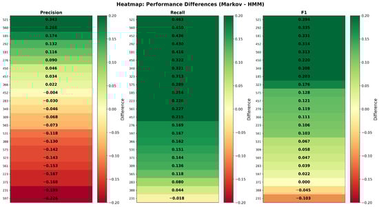
Figure 19. Heatmap visualization of performance differences (Markov Chain minus HMM) across all vehicles for precision, recall, and F1-score. Vehicles are ranked by difference magnitude. Green indicates Markov superiority, red indicates HMM superiority, and yellow indicates near-equivalent performance.

6. Discussion

The results are consolidated in Table 11, which presents the mean precision values and statistical significance for each vehicle. Out of 23 vehicles analyzed, 18 (78.3%) exhibited statistically significant differences between Markov Chain and HMM precision values (p < 0.05). Five vehicles (283, 340, 366, 452, and 457) displayed no statistically significant differences. The maximum observed difference was slightly below 5% for vehicle 340, while vehicle 452 displayed a variation of less than 1%. These results validate the filtering threshold of 50 trajectories employed in this study. Values below this threshold consistently reduced average precision in preliminary experiments and were therefore excluded from the analysis.

To provide a more comprehensive assessment of model performance, the analysis was extended to include recall and F1-score alongside precision, as shown in Figure 15. While the HMM demonstrated marginally superior precision (0.6101 vs. 0.5908, p = 0.0248), the Markov Chain model significantly outperformed the HMM in both recall (0.6829 vs. 0.4430, p < 0.0001) and F1-score (0.6148 vs. 0.4727, p < 0.0001). The cases where Markov chains achieved superior recall and F1-score compared to HMMs are due to inherent limitations in the HMM architecture regarding the day of the week and origin grid (origin grid tag), which filter the results making the probabilities more restricted. For example, if previously there would be X possibilities across the 7 days of the week, now there are Y possibilities for Wednesdays, where Y equals X minus the other 6 days of the week. This filtering effect constrains the HMM’s prediction coverage, resulting in lower recall despite higher precision.

It is important to note that the recall and F1-score metrics, in this specific context, may not fully represent the practical performance of the HMM approach. The architectural filtering imposed by conditioning on day of the week systematically reduces the set of possible predicted destinations, which artificially deflates recall values. This does not necessarily indicate inferior predictive capability, but rather reflects a more conservative prediction strategy where the model abstains from predictions when insufficient contextual evidence is available. In operational scenarios where prediction confidence is prioritized over coverage, this conservative behavior may actually be advantageous. Therefore, the observed lower recall and F1-score should be interpreted as a consequence of the HMM’s restrictive design choice rather than as an absolute measure of model quality.

The statistical parity across the five vehicles with non-significant differences suggests that both algorithms process trajectory data similarly under the tested conditions for those specific cases. The observed variations in precision, ranging from less than 1% to slightly below 5%, likely reflect differences in how each algorithm interprets individual vehicle movement patterns rather than systematic performance advantages. However, the multi-metric analysis reveals a fundamental trade-off: HMMs achieve higher precision on average but at the cost of substantially lower recall and F1-score compared to Markov chains.

HMM inherently incorporates contextual information that aligns with the temporal and spatial dimensions of human movement behavior. Consequently, model selection should not rely exclusively on quantitative precision metrics. The choice between techniques must consider the specific characteristics of each dataset, the nature of the phenomena under investigation, the balance between prediction accuracy and coverage, and the intended predictive objectives related to human mobility patterns.

These findings gain practical relevance when considered within the context of real-world urban mobility applications, particularly in IoT-based systems. The growing integration of IoT systems in urban mobility environments [59] reinforces the importance of robust predictive methods for route optimization and real-time traffic management. IoT-based architectures that integrate heterogeneous sensing with edge-cloud processing demonstrate potential for reducing congestion and emissions, especially when combined with algorithms capable of anticipating vehicular movement patterns. In this context, the choice between predictive techniques such as Markov and HMM becomes even more relevant, as routing decisions in intelligent transportation systems fundamentally depend on the precision, coverage, and efficiency of the employed models.

The analysis of large-scale mobility data, as demonstrated by recent studies using smart card data [1], reveals that different user profiles (high and low frequency) distinctly impact the structure and robustness of transportation networks. Analogously, the vehicular trajectory patterns analyzed in this study also reveal behavioral heterogeneity that may influence the performance of predictive algorithms. The segmentation by route repetition frequency (threshold of 50 trajectories) aligns with this perspective, as vehicles with more regular patterns tend to exhibit greater predictability, similarly to what is observed in public transportation networks with high-frequency users.

These findings indicate the need for future research incorporating contextual and semantic data to fully assess model capabilities, especially considering the growing availability of data from urban IoT ecosystems. The integration of multiple heterogeneous data sources (traffic sensors, weather conditions, urban events, and historical patterns) can significantly enrich the predictive capacity of both models. Future work should also explore the incorporation of richer spatiotemporal features beyond day of the week, which could potentially allow the structural advantages of HMMs to be leveraged without suffering from excessive data sparsity. Nonetheless, the developed method provides a suitable framework for investigating how the sample data structure influences predictive algorithm performance, contributing to the development of more intelligent and sustainable transportation systems.

Within this framework, the present study addresses specific gaps in the trajectory prediction literature through systematic comparative evaluation using identical training data, tessellation parameters, and cross-validation protocols. The analysis reveals an underexplored precision–coverage trade-off: HMMs achieve marginally higher precision (61.01% vs. 59.08%, p = 0.0248) but significantly lower recall (44.30% vs. 68.29%, p < 0.0001) and F1-score (47.27% vs. 61.48%, p < 0.0001). This 24-percentage-point recall deficit demonstrates that HMM’s contextual filtering (conditioning on day-of-week observations) restricts prediction coverage despite improving precision.

By incorporating precision, recall, and F1-score alongside 10-fold cross-validation and paired t-tests, the multi-metric evaluation exposes that aggregate precision metrics can mask substantial differences in operational coverage. This distinction is critical for IoT deployment: applications prioritizing service breadth (e.g., proactive route recommendation) may favor Markov Chains, while safety-critical systems requiring high confidence may accept HMM’s restricted coverage. Furthermore, the SSDF method’s 50-trajectory threshold, while ensuring statistical robustness, disproportionately affects vehicles with irregular patterns, as evidenced by Markov Chains outperforming HMMs for vehicles 181, 292, and 450. This filtering-induced bias, rarely quantified in the existing literature, has direct implications for model fairness across heterogeneous user populations.

Comparison with Recent Approaches

To contextualize these findings within the current landscape of trajectory and destination prediction research, Table 12 presents a systematic comparison with 11 recent studies published between 2023 and 2025. As demonstrated, existing approaches employ heterogeneous metrics measuring distinct aspects of predictive quality: spatial distance-based metrics (RMSE, ADE, FDE), sequence matching rates (CMP), and classification metrics (Accuracy, Precision, Recall, F1, AUC, Kappa).

Table 12. Comparative Analysis of Recent Trajectory and Destination Prediction Studies.

Study Title	Ref.	Year	Method/Dataset	Metrics	Results
Urban Travel Chain CHMM-LDA	[60]	2025	CHMM-LDA a/Seoul	P m, R n, F1 o	P = 81.3%, R = 80.1%, F1 = 81.2%
Markov Chain Transportation	[61]	2025	Grey-Markov/Badajoz	RMSE p	$E_m$  q$< 10\%$
Vehicle Trajectory LSTM-Attn	[62]	2025	LSTM + Attn b/NGSIM c	RMSE, ADE r, FDE s	2.15 m, 0.67 m, 1.52 m
Trajectory Planning POMDP	[63]	2023	POMDP + DQN d/Lyft	Safety, Energy	+2.5%, $-42\%$
Map Matching HMM-CRFs	[64]	2024	HMM-CRFs e/Guangzhou	CMP f	96.4%
Trajectory Urban Network	[22]	2023	UTA g/Hangzhou	AUC t, RMSE	95.5%, 600 m
Traffic Status 2nd-HMM	[65]	2023	2nd-order HMM/Shenzhen	Accuracy	88.9%
Knowledge Graph HMM	[66]	2025	KHMM h/Changsha	POI u popularity	High quality
Testing 1st-HMMs Mobility	[67]	2024	1st-order HMM/Borlange	Accuracy	POI > 75%, Time > 70%
Pedestrian Accident CA-MC	[68]	2023	CA-MC i + LRM/Mashhad	Kappa v, ROC w	0.94, 0.88
Trajectory Bayesian Net	[69]	2023	DBNTP j/Simulator	Lat. error x	T y = 2 s: 0.69 m
This Work with MC vs. HMM	-	2025	SSDF k/VED l	P, R, F1	MC: 59/68/61; HMM: 61/44/47

^a CHMM: Continuous Hidden Markov Model; LDA: Latent Dirichlet Allocation. ^b Attn: Attention mechanism; LSTM: Long Short-Term Memory network. ^c NGSIM: Next Generation Simulation dataset (US Federal Highway Administration). ^d POMDP: Partially Observable Markov Decision Process; DQN: Deep Q-Network. ^e CRFs: Conditional Random Fields. ^f CMP: Correct Matching Percentage. ^g UTA: Urban Topology-encoding Attention Network. ^h KHMM: Knowledge Graph-based Hidden Markov Model. ⁱ CA-MC: Cellular Automata Markov Chain; LRM: Logistic Regression Model. ^j DBNTP: Dynamic Bayesian Network Trajectory Prediction. ^k SSDF: Smart Sampling with Data Filtering (proposed method in this work). ^l VED: Vehicle Energy Dataset (Ann Arbor, Michigan; 23 vehicles, November 2017–November 2018). ^m P: Precision, calculated as $\mathrm{P}={\displaystyle \frac{\mathrm{TP}}{\mathrm{TP}+\mathrm{FP}}}$ where $\mathrm{TP}$ = True Positives, $\mathrm{FP}$ = False Positives. ⁿ R: Recall, calculated as $\mathrm{R}={\displaystyle \frac{\mathrm{TP}}{\mathrm{TP}+\mathrm{FN}}}$ where $\mathrm{FN}$ = False Negatives. ^o F1: F1-score (harmonic mean of Precision and Recall), $\mathrm{F}1=2\times {\displaystyle \frac{\mathrm{P}\times \mathrm{R}}{\mathrm{P}+\mathrm{R}}}$. ^p RMSE: Root Mean Squared Error, $\mathrm{RMSE}=\sqrt{{\displaystyle \frac{1}{n}}{\sum }_{i=1}^n{(y_i-{\widehat{y}}_i)}^2}$. ^q $E_m$: Mean relative error. ^r ADE: Average Displacement Error (mean Euclidean distance across all predicted timesteps). ^s FDE: Final Displacement Error (Euclidean distance at final prediction timestep). ^t AUC: Area Under the Curve (ROC curve metric). ^u POI: Point of Interest (geographic locations of user activity). ^v Kappa: Cohen’s Kappa coefficient (inter-rater agreement statistic). ^w ROC: Receiver Operating Characteristic (curve showing true positive vs. false positive rates). ^x Lat. error: Lateral error (perpendicular distance from predicted to actual trajectory). ^y T: Time horizon for prediction.

Probabilistic and machine learning methods demonstrate diverse performance profiles across trajectory and destination prediction tasks: Xiao et al. [60] achieved F1-scores of 81.2% for urban travel chains using CHMM-LDA on Seoul mobility data; Li et al. [61] reported mean errors below 10% using Grey-Markov models for transportation forecasting in Badajoz; Wang et al. [62] obtained RMSE of 2.15 m in vehicular trajectory prediction with LSTM and attention mechanisms on NGSIM; Zhang et al. [63] achieved 2.5% safety improvement and 42% energy reduction using POMDP with deep reinforcement learning on Lyft data; Qin et al. [22] obtained AUC of 95.5% with urban topology-encoding networks on Hangzhou trajectories; and Jiang et al. [69] reported 0.69 m lateral error at 2-s prediction horizons using dynamic Bayesian networks in simulated environments.

Complementary applications in map matching, traffic status recognition, and spatial analytics further illustrate the breadth of Markovian approaches: Li et al. [64] attained 96.4% correct matching in map matching using HMM-CRFs on Guangzhou taxi GPS; Li et al. [65] reported 88.9% accuracy in traffic status recognition using second-order HMMs on Shenzhen probe data; Zeng et al. [66] demonstrated high-quality POI predictions through knowledge graph-enhanced HMMs on Changsha mobility; Sadeghian et al. [67] achieved over 75% POI accuracy and 70% temporal accuracy with first-order HMMs on Borlange GPS data; and Mohammadi et al. [68] obtained Kappa of 0.94 and ROC of 0.88 for pedestrian accident prediction using cellular automata Markov chains in Mashhad.

However, direct numerical comparison across these studies is infeasible due to heterogeneity in prediction objectives (final destination vs. complete trajectory vs. map matching vs. traffic status vs. safety events), datasets (scales ranging from dozens to tens of thousands of trajectories across diverse urban contexts and data sources), and evaluation frameworks (distance-based vs. classification-based vs. probabilistic metrics). This work distinguishes itself by explicitly quantifying the fundamental precision–coverage trade-off through multi-metric evaluation (Precision, Recall, F1-score) under controlled experimental conditions with 10-fold cross-validation. Results reveal that contextual integration via HMM marginally improves precision (61.01% vs. 59.08%, p = 0.0248), yet substantially reduces recall (44.30% vs. 68.29%, p < 0.0001) and F1-score (47.27% vs. 61.48%, p < 0.0001), demonstrating that architectural filtering imposed by day-of-week conditioning restricts predictive coverage. This explicit precision–coverage trade-off analysis, which remains absent in the compared literature, provides actionable guidance for model selection based on application-specific requirements in vehicular IoT systems.

7. Conclusions and Future Work

This study contributes to the ongoing transformation of urban environments into IoT-driven Smart Cities by demonstrating how interpretable probabilistic models can enhance intelligent mobility. By leveraging real-world vehicular IoT data, the proposed framework supports data-driven decision-making for sustainable traffic management and energy efficiency. The integration of lightweight predictive models such as Markov Chains and Hidden Markov Models aligns with the growing demand for explainable solutions that are deployable at the edge of IoT infrastructures. In this context, the findings reinforce the importance of designing transparent analytical pipelines capable of operating under real-time and resource-constrained conditions, thus advancing the broader goal of intelligent and sustainable urban mobility.

Therefore, this research presented a comparative analysis between Markov Chains and Hidden Markov Models for destination prediction in urban vehicular contexts. The developed SSDF method provides a statistically rigorous framework for evaluating Markovian approaches to trajectory prediction, contributing to the understanding of how different algorithms process urban mobility patterns. Importantly, the multi-metric evaluation revealed fundamental trade-offs between prediction accuracy and coverage that must be considered when selecting appropriate models for real-world deployment.

The potential impact of the proposed approach can be exemplified in a Smart City traffic management context. Imagine an urban control center that aggregates IoT data streams from vehicles, smart traffic lights, and roadside units [70,71]. Using the SSDF methodology with Markovian predictors, the system could identify recurrent destination patterns at different times of day and predict congestion zones minutes before they occur. Such predictive capability would enable the city’s control algorithms to dynamically adjust signal phases, optimize public transport routes, and even provide personalized route suggestions to drivers. The choice between Markov Chains and HMMs in such systems would depend on operational priorities: Markov Chains offer broader coverage and consistent predictions across diverse scenarios, while HMMs provide higher confidence predictions within more restricted contexts. Beyond improving traffic flow, this approach could also support environmental monitoring initiatives by correlating predicted routes with energy consumption and estimated emissions, contributing to data-driven sustainability policies. In light of these practical implications and the demonstrated potential of the proposed framework for IoT-driven mobility systems, the main contributions of this work are summarized as follows:

• A comprehensive multi-metric comparison demonstrating that while HMM achieved marginally higher precision (61.01% vs. 59.08%, p = 0.0248), Markov Chains significantly outperformed HMMs in recall (68.29% vs. 44.30%, p < 0.0001) and F1-score (61.48% vs. 47.27%, p < 0.0001) when incorporating day-of-week contextual information, with statistically significant differences observed in 78.3% of the 23-vehicle sample across precision metrics.
• Identification of a fundamental architectural trade-off, where HMM’s contextual filtering (day-of-week + origin grid) constrains prediction coverage despite improving precision; revealing that if there would be X destination possibilities across all weekdays, conditioning on specific weekdays reduces available options to Y (where Y equals X minus the other 6 days), thus explaining the substantially lower recall observed in HMM predictions.
• An automatic threshold selection algorithm (Algorithm 1) balancing statistical adequacy with data retention, determining 50 trajectory sequences per vehicle as optimal for both model types.
• A replicable methodological pipeline encompassing trajectory segmentation, spatial tessellation, frequency aggregation, and 10-fold cross-validation which is suitable for diverse trajectory datasets, with multi-metric evaluation protocols that reveal performance trade-offs beyond single-metric assessments.
• Evidence of statistical parity between models in precision for 21.7% of cases (5 of 23 vehicles), indicating that model selection criteria should consider the trade-off between contextual awareness, prediction coverage, and computational simplicity when evaluating potential applications in resource-constrained environments.

As a future research direction, this work can be extended by exploring advanced probabilistic and hybrid learning strategies that operate on streaming or edge-based IoT environments. Building upon the statistical insights and the method established in this study, such extensions could enhance trajectory prediction accuracy while maintaining efficiency and interpretability in real-time urban mobility systems.

Enhanced contextual feature integration. Expanding beyond day-of-week to incorporate time-of-day, weekend indicators, holidays, weather conditions, and traffic density could reveal more substantial performance differentials between models. Crucially, richer spatiotemporal features could potentially allow the structural advantages of HMMs to be leveraged without suffering from excessive data sparsity, addressing the coverage limitations identified in this study. This would provide deeper insights into how contextual enrichment influences the precision–recall trade-off across varying urban mobility scenarios.

Adaptive spatial discretization. Developing hierarchical tessellation methods that adjust resolution based on trajectory density and urban characteristics could improve prediction accuracy while maintaining computational feasibility. Variable-resolution grids could better capture both dense urban cores and sparse suburban areas within unified frameworks.

Extended dataset validation. Application of the SSDF method to publicly available trajectory datasets (GeoLife, T-Drive, others) could help to assess generalizability across different geographical regions, cultural contexts, and transportation patterns. Cross-dataset validation with multi-metric evaluation would strengthen confidence in the methodological approach and reveal dataset-specific characteristics that influence model performance trade-offs.

Computational efficiency analysis. Systematic evaluation of processing time, memory requirements, and prediction latency for both models across varying sample sizes would inform practical deployment considerations. Understanding computational trade-offs becomes particularly relevant when considering applications in environments with limited processing capabilities, such as edge computing scenarios in emerging smart mobility systems [59].

Hybrid modeling approaches. Investigating ensemble methods that combine Markov Chain efficiency and broad coverage for stable patterns with HMM contextual awareness for variable conditions could optimize the precision–coverage–complexity balance. Adaptive switching mechanisms between models based on detected pattern regularity and available contextual information merit exploration.

Coverage-aware evaluation frameworks. Developing evaluation methodologies that explicitly account for prediction abstention rates and context-dependent performance would provide more nuanced assessments of model behavior in operational settings. This includes investigating scenarios where conservative prediction strategies (higher precision, lower coverage) are preferable to aggressive strategies (higher coverage, lower precision).

Fairness and explainability in IoT mobility analytics. Building upon prior advances in fairness-aware and explainable modeling for streaming data [10,71], future work could explore how such principles apply to trajectory prediction in IoT-enabled urban environments. This direction involves assessing whether model interpretability and equitable performance vary across different vehicle or region profiles, promoting more transparent and socially responsible Smart City mobility systems.

Behavioral segmentation refinement. Following insights from recent mobility pattern analysis [1], this line of research involves examining how trajectory frequency categories (high, medium, low repetition) differentially influence model performance could enable more targeted prediction strategies. Vehicles exhibiting regular commuting patterns may benefit from simpler models with broader coverage, while those with variable routes might require contextual modeling despite reduced coverage.

These directions maintain focus on rigorous statistical evaluation of Markovian approaches while gradually extending the framework toward real-world applicability. The SSDF method provides a foundation for investigating how trajectory data structure, contextual enrichment, and algorithmic complexity interact to influence prediction performance trade-offs. Future work bridging offline statistical analysis with operational deployment scenarios would require careful validation of computational constraints, real-time data integration capabilities, and scalability considerations. These challenges extend beyond the scope of this comparative study but represent natural progressions of the established methodology.

References

- Sun, L.; Ashrafi, N.; Pishgar, M. Optimizing Urban Mobility Through Complex Network Analysis and Big Data from Smart Cards. IoT 2025, 6, 44. [Google Scholar] [CrossRef]
- Araújo, T.; Cappiello, C.; Kozievitch, N.; Mestre, D.; Santos Pires, C.; Vitali, M. Towards Reliable Data Analyses for Smart Cities. In Proceedings of the 21st International Database Engineering & Applications Symposium, IDEAS ’17, Bristol, UK, 12–14 July 2017; pp. 304–308. [Google Scholar] [CrossRef]
- Kandt, J.; Batty, M. Smart cities, big data and urban policy: Towards urban analytics for the long run. Cities 2021, 109, 102992. [Google Scholar] [CrossRef]
- Semanjski, I.C. Smart Urban Mobility: Transport Planning in the Age of Big Data and Digital Twins; Elsevier: Amsterdam, The Netherlands, 2023. [Google Scholar]
- Jeremiah, S.R.; Yang, L.T.; Park, J.H. Digital twin-assisted resource allocation framework based on edge collaboration for vehicular edge computing. Future Gener. Comput. Syst. 2024, 150, 243–254. [Google Scholar] [CrossRef]
- Alalwany, E.; Mahgoub, I. Security and Trust Management in the Internet of Vehicles (IoV): Challenges and Machine Learning Solutions. Sensors 2024, 24, 368. [Google Scholar] [CrossRef]
- Khezri, E.; Hassanzadeh, H.; Yahya, R.O.; Mir, M. Security Challenges in Internet of Vehicles (IoV) for ITS: A Survey. Tsinghua Sci. Technol. 2025, 30, 1700–1723. [Google Scholar] [CrossRef]
- Ramírez-Moreno, M.A.; Keshtkar, S.; Padilla-Reyes, D.A.; Ramos-Lopez, E.; García Martínez, M.; Hernandez-Lunas, M.; Mogro, A.E.; Mahlknecht, J.; Huertas, J.I.; Peimbert-García, R.E.; et al. Sensors for Sustainable Smart Cities: A Review. Appl. Sci. 2021, 11, 8198. [Google Scholar] [CrossRef]
- Rizwan, P.; Suresh, K.; Babu, M.R. Real-time smart traffic management system for smart cities by using Internet of Things and big data. In Proceedings of the 2016 International Conference on Emerging Technological Trends (ICETT), Kollam, India, 21–22 October 2016; IEEE: Piscataway, NJ, USA, 2016; pp. 1–7. [Google Scholar] [CrossRef]
- Araújo, T.B.; Efthymiou, V.; Stefanidis, K. Fairness and Explanations in Entity Resolution: An Overview. IEEE Access 2025, 13, 145127–145143. [Google Scholar] [CrossRef]
- Norris, J.R. Markov Chains; Cambridge Series in Statistical and Probabilistic Mathematics; Cambridge University Press: Cambridge, UK, 1998. [Google Scholar]
- Eddy, S.R. What is a hidden Markov model? Nat. Biotechnol. 2004, 22, 1315–1316. [Google Scholar] [CrossRef]
- Yang, H.; Zhang, X.; Li, Z.; Cui, J. Region-level traffic prediction based on temporal multi-spatial dependence graph convolutional network from GPS data. Remote Sens. 2022, 14, 303. [Google Scholar] [CrossRef]
- Molina-Campoverde, J.J.; Rivera-Campoverde, N.; Molina Campoverde, P.A.; Bermeo Naula, A.K. Urban mobility pattern detection: Development of a classification algorithm based on machine learning and GPS. Sensors 2024, 24, 3884. [Google Scholar] [CrossRef]
- Merenda, M.; Porcaro, C.; Iero, D. Edge Machine Learning for AI-Enabled IoT Devices: A Review. Sensors 2020, 20, 2533. [Google Scholar] [CrossRef] [PubMed] [PubMed Central]
- Kitchenham, B.; Charters, S. Guidelines for Performing Systematic Literature Reviews in Software Engineering; Keele University: Keele, UK; University of Durham: Durham, UK, 2007. [Google Scholar]
- Firmino Junior, J.B.; Dutra, J.F.; Neto, F.D.N. Evaluation of trajectory and destination prediction models: A systematic classification and analysis of methodologies and recent results. J. Internet Serv. Appl. 2024, 11, 474–484. [Google Scholar] [CrossRef]
- Wang, Z.; Guo, J.; Hu, Z.; Zhang, H.; Zhang, J.; Pu, J. Lane Transformer: A High-Efficiency Trajectory Prediction Model. IEEE Open J. Intell. Transp. Syst. 2023, 4, 2–13. [Google Scholar] [CrossRef]
- Sadri, A.; Salim, F.D.; Ren, Y.; Shao, W.; Krumm, J.C.; Mascolo, C. What Will You Do for the Rest of the Day? An Approach to Continuous Trajectory Prediction. Proc. ACM Interact. Mob. Wearable Ubiquitous Technol. 2018, 2, 1–26. [Google Scholar] [CrossRef]
- Dai, S.; Li, L.; Li, Z. Modeling Vehicle Interactions via Modified LSTM Models for Trajectory Prediction. IEEE Access 2019, 7, 38287–38296. [Google Scholar] [CrossRef]
- Lassoued, Y.; Monteil, J.; Gu, Y.; Russo, G.; Shorten, R.; Mevissen, M. A hidden Markov model for route and destination prediction. In Proceedings of the 2017 IEEE 20th International Conference on Intelligent Transportation Systems (ITSC), Yokohama, Japan, 16–19 October 2017. [Google Scholar] [CrossRef]
- Qin, X.; Li, Z.; Zhang, K.; Mao, F.; Jin, X. Vehicle Trajectory Prediction via Urban Network Modeling. Sensors 2023, 23, 4893. [Google Scholar] [CrossRef]
- Santana, A.V.; Campos, J. Travel History: Reconstructing Semantic Trajectories Based on Heterogeneous Social Tracks Sources. In Proceedings of the 22nd Brazilian Symposium on Multimedia and the Web, Webmedia ’16, Teresina Piauí, Brazil, 8–11 November 2016. [Google Scholar] [CrossRef]
- Shen, G.; Li, P.; Chen, Z.; Yang, Y.; Kong, X. Spatio-temporal interactive graph convolution network for vehicle trajectory prediction. Internet Things 2023, 24, 100935. [Google Scholar] [CrossRef]
- Taslimasa, H.; Dadkhah, S.; Neto, E.C.P.; Xiong, P.; Ray, S.; Ghorbani, A.A. Security Issues in Internet of Vehicles (IoV): A Comprehensive Survey. Internet Things 2023, 22, 100809. [Google Scholar] [CrossRef]
- Xu, C.; Zhang, P.; Xia, X.; Kong, L.; Zeng, P.; Yu, H. Digital-Twin-Assisted Intelligent Secure Task Offloading and Caching in Blockchain-Based Vehicular Edge Computing Networks. IEEE Internet Things J. 2025, 12, 4128–4143. [Google Scholar] [CrossRef]
- Druck, S.; Carvalho, M.S.; Câmara, G.; Monteiro, A.V.M. Análise espacial de dados geográficos; Embrapa: Brasília, Brazil, 2004. [Google Scholar]
- Zheng, Y. Trajectory Data Mining: An Overview. ACM Trans. Intell. Syst. Technol. 2015, 6, 29:1–29:41. [Google Scholar] [CrossRef]
- Yan, Z.; Chakraborty, D.; Parent, C.; Spaccapietra, S.; Aberer, K. Semantic Trajectories: Mobility Data Computation and Annotation. ACM Trans. Intell. Syst. Technol. 2013, 4, 1–38. [Google Scholar] [CrossRef]
- Gold, C. Tessellations in GIS: Part I—Putting It All Together. Geo-Spat. Inf. Sci. 2016, 19, 9–25. [Google Scholar] [CrossRef]
- Okabe, A.; Boots, B.; Sugihara, K.; Chiu, S.N. Spatial Tessellations: Concepts and Applications of Voronoi Diagrams, 2nd ed.; John Wiley & Sons: Chichester, UK, 2000. [Google Scholar] [CrossRef]
- Aurenhammer, F. Voronoi Diagrams—A Survey of a Fundamental Geometric Data Structure. ACM Comput. Surv. 1991, 23, 345–405. [Google Scholar] [CrossRef]
- Ortúzar, J.d.D.; Willumsen, L.G. Modelling Transport, 4th ed.; John Wiley & Sons: Chichester, UK, 2011. [Google Scholar]
- Sun, Y.; Meng, F.; Li, R.; Tang, Y.; Chen, C.; Zhong, J. Streaming trajectory segmentation based on stay-point detection. In Proceedings of the Database Systems for Advanced Applications, Gifu, Japan, 2–5 July 2024; Springer Nature: Cham, Switzerland, 2024; Volume 14850. [Google Scholar]
- Li, Q.; Zheng, Y.; Xie, X.; Chen, Y.; Liu, W.; Ma, W.Y. Mining User Similarity Based on Location History. In Proceedings of the 16th ACM SIGSPATIAL International Conference on Advances in Geographic Information Systems (GIS ’08), Irvine, CA, USA, 5–7 November 2008; ACM: New York, NY, USA, 2010; pp. 34:1–34:10. [Google Scholar] [CrossRef]
- Palma, A.T.; Bogorny, V.; Kuijpers, B.; Alvares, L.O. A Clustering-Based Approach for Discovering Interesting Places in Trajectories. In Proceedings of the 2008 ACM Symposium on Applied Computing (SAC ’08), Fortaleza, Brazil, 16–20 March 2008; ACM: New York, NY, USA, 2008; pp. 863–868. [Google Scholar] [CrossRef]
- Meyn, S.P.; Tweedie, R.L. Markov Chains and Stochastic Stability, 2nd ed.; Cambridge University Press: Cambridge, UK, 2009. [Google Scholar] [CrossRef]
- Ching, W.K.; Ng, M.K. Markov Chains: Models, Algorithms and Applications; International Series in Operations Research & Management Science; Springer Science & Business Media: Berlin/Heidelberg, Germany, 2006; Volume 83. [Google Scholar]
- Stewart, W.J. Probability, Markov Chains, Queues, and Simulation: The Mathematical Basis of Performance Modeling; Princeton University Press: Princeton, NJ, USA, 2009. [Google Scholar] [CrossRef]
- Stamp, M. Introduction to Machine Learning with Applications in Information Security, 2nd ed.; Chapman and Hall/CRC: Boca Raton, FL, USA, 2018. [Google Scholar] [CrossRef]
- Bilmes, J.A. A Gentle Tutorial of the EM Algorithm and Its Application to Parameter Estimation for Gaussian Mixture and Hidden Markov Models; Technical Report TR-97-021; International Computer Science Institute, University of California at Berkeley: Berkeley, CA, USA, 1998. [Google Scholar]
- Dempster, A.P.; Laird, N.M.; Rubin, D.B. Maximum Likelihood from Incomplete Data via the EM Algorithm. J. R. Stat. Soc. Ser. B (Methodol.) 1977, 39, 1–22. [Google Scholar] [CrossRef]
- Grewal, J.K.; Krzywinski, M.; Altman, N. Markov models—Hidden Markov models. Nat. Methods 2019, 16, 795–796. [Google Scholar] [CrossRef]
- Forney, G.D. The Viterbi Algorithm. Proc. IEEE 1973, 61, 268–278. [Google Scholar] [CrossRef]
- Rabiner, L.R. A Tutorial on Hidden Markov Models and Selected Applications in Speech Recognition. Proc. IEEE 1989, 77, 257–286. [Google Scholar] [CrossRef]
- Ephraim, Y.; Merhav, N. Hidden Markov Processes. IEEE Trans. Inf. Theory 2002, 48, 1518–1569. [Google Scholar] [CrossRef]
- Durbin, R.; Eddy, S.R.; Krogh, A.; Mitchison, G. Biological Sequence Analysis: Probabilistic Models of Proteins and Nucleic Acids; Cambridge University Press: Cambridge, UK, 1998. [Google Scholar]
- Batista, G.E.; Prati, R.C.; Monard, M.C. A Study of the Behavior of Several Methods for Balancing Machine Learning Training Data. ACM SIGKDD Explor. Newsl. 2004, 6, 20–29. [Google Scholar] [CrossRef]
- He, H.; Garcia, E.A. Learning from Imbalanced Data. IEEE Trans. Knowl. Data Eng. 2009, 21, 1263–1284. [Google Scholar] [CrossRef]
- Anderson, T.W.; Goodman, L.A. Statistical Inference about Markov Chains. Ann. Math. Statist. 1957, 28, 89–110. [Google Scholar] [CrossRef]
- Koski, T. Hidden Markov Models for Bioinformatics; Computational Biology; Springer Science & Business Media: Berlin/Heidelberg, Germany, 2001; Volume 2. [Google Scholar]
- Bishop, C.M. Pattern Recognition and Machine Learning; Information Science and Statistics; Springer: New York, NY, USA, 2006. [Google Scholar]
- Oh, G. VED GitHub Repository. 2022. Available online: https://github.com/gsoh/VED (accessed on 13 September 2025).
- Oh, G.; Leblanc, D.J.; Peng, H. Vehicle Energy Dataset (VED), A Large-Scale Dataset for Vehicle Energy Consumption Research. IEEE Trans. Intell. Transp. Syst. 2022, 23, 3302–3312. [Google Scholar] [CrossRef]
- Graser, A. MovingPandas: Efficient Structures for Movement Data in Python. GI Forum J. Geogr. Inf. Sci. 2019, 7, 54–68. [Google Scholar] [CrossRef]
- Graser, A.; MovingPandas Team. MovingPandas. Python Library for Trajectory Data Manipulation. 2024. Available online: https://movingpandas.org (accessed on 7 October 2025).
- Froehlich, J.; Krumm, J. Route Prediction from Trip Observations; SAE Technical Paper 2008-01-0201; SAE International: Warrendale, PA, USA, 2008. [Google Scholar] [CrossRef]
- Sirqueira, T.F.M.; Miguel, M.A.; Dalpra, H.L.O.; Araujo, M.A.P.; David, J.M.N. Application of Statistical Methods in Software Engineering: Theory and Practice. arXiv 2020, arXiv:2006.15624. Available online: https://arxiv.org/abs/2006.15624 (accessed on 4 October 2025). [CrossRef]
- Reis, M.J.C.S.; Branco, F.; Gupta, N.; Serôdio, C. An IoT Architecture for Sustainable Urban Mobility: Towards Energy-Aware and Low-Emission Smart Cities. Future Internet 2025, 17, 457. [Google Scholar] [CrossRef]
- Xiao, C.; Tang, J.; Lee, J.J.; Liang, Y. Urban Travel Chain Estimation Based on Combination of CHMM and LDA Model. IET Intell. Transp. Syst. 2025, 19, e70004. [Google Scholar] [CrossRef]
- Li, X. Study on the Application of Markov Chains in Transportation. Theor. Nat. Sci. 2025, 100, 171–178. [Google Scholar] [CrossRef]
- Wang, T.; Fu, Y.; Cheng, X.; Li, L.; He, Z.; Xiao, Y. Vehicle Trajectory Prediction Algorithm Based on Hybrid Prediction Model with Multiple Influencing Factors. Sensors 2025, 25, 1024. [Google Scholar] [CrossRef]
- Zhang, E.; Zhang, R.; Masoud, N. Predictive Trajectory Planning for Autonomous Vehicles at Intersections Using Reinforcement Learning. Transp. Res. Part C Emerg. Technol. 2023, 149, 104063. [Google Scholar] [CrossRef]
- Li, W.; Chen, Y.; Wang, S.; Li, H.; Fan, Q. A Novel Map Matching Method Based on Improved Hidden Markov and Conditional Random Fields Model. Int. J. Digit. Earth 2024, 17, 2328366. [Google Scholar] [CrossRef]
- Li, F.; Liu, K.; Chen, J. Traffic Status Prediction Based on Multidimensional Feature Matching and 2nd-Order Hidden Markov Model (HMM). Sustainability 2023, 15, 14671. [Google Scholar] [CrossRef]
- Zeng, Z.; Qin, J.; Wu, T. A Knowledge Graph-Enhanced Hidden Markov Model for Personalized Travel Routing: Integrating Spatial and Semantic Data in Urban Environments. Smart Cities 2025, 8, 75. [Google Scholar] [CrossRef]
- Sadeghian, P.; Han, M.; Håkansson, J.; Zhao, M.X. Testing Feasibility of Using a Hidden Markov Model on Predicting Human Mobility Based on GPS Tracking Data. Transp. B Transp. Dyn. 2024, 12, 2336037. [Google Scholar] [CrossRef]
- Mohammadi, A.; Kiani, B.; Mahmoudzadeh, H.; Bergquist, R. Pedestrian Road Traffic Accidents in Metropolitan Areas: GIS-Based Prediction Modelling of Cases in Mashhad, Iran. Sustainability 2023, 15, 10576. [Google Scholar] [CrossRef]
- Jiang, Y.; Zhu, B.; Yang, S.; Zhao, J.; Deng, W. Vehicle Trajectory Prediction Considering Driver Uncertainty and Vehicle Dynamics Based on Dynamic Bayesian Network. IEEE Trans. Syst. Man Cybern. Syst. 2023, 53, 689–703. [Google Scholar] [CrossRef]
- Araújo, T.B.; Stefanidis, K.; Pires, C.E.S.; Nummenmaa, J.; da Nóbrega, T.P. Incremental entity blocking over heterogeneous streaming data. Information 2022, 13, 568. [Google Scholar] [CrossRef]
- Araújo, T.B.; Efthymiou, V.; Christophides, V.; Pitoura, E.; Stefanidis, K. TREATS: Fairness-aware entity resolution over streaming data. Inf. Syst. 2025, 129, 102506. [Google Scholar] [CrossRef]
Disclaimer/Publisher’s Note: The statements, opinions and data contained in all publications are solely those of the individual author(s) and contributor(s) and not of MDPI and/or the editor(s). MDPI and/or the editor(s) disclaim responsibility for any injury to people or property resulting from any ideas, methods, instructions or products referred to in the content. |
© 2025 by the authors. Licensee MDPI, Basel, Switzerland. This article is an open access article distributed under the terms and conditions of the Creative Commons Attribution (CC BY) license (https://creativecommons.org/licenses/by/4.0/).