Urban Traffic Congestion Prediction: A Multi-Step Approach Utilizing Sensor Data and Weather Information

Abstract

The continuous growth of urban populations has led to the persistent problem of traffic congestion, which imposes adverse effects on quality of life, such as commute times, road safety, and the local air quality. Advancements in Internet of Things (IoT) sensor technology have contributed to a plethora of new data streams regarding traffic conditions. Therefore, the recognition and prediction of traffic congestion patterns utilizing such data have become crucial. To that end, the integration of Machine Learning (ML) algorithms can further enhance Intelligent Transportation Systems (ITS), contributing to the smart management of transportation systems and effectively tackling traffic congestion in cities. This study seeks to assess a wide range of models as potential solutions for an ML-based multi-step forecasting approach intended to improve traffic congestion prediction, particularly in areas with limited historical data. Various interpretable predictive algorithms, suitable for handling the complexity and spatiotemporal characteristics of urban traffic flow, were tested and eventually shortlisted based on their predictive performance. The forecasting approach selects the optimal model in each step to maximize the accuracy. The findings demonstrate that, in a 24 h step prediction, variating Ensemble Tree-Based (ETB) regressors like the Light Gradient Boosting Machine (LGBM) exhibit superior performances compared to traditional Deep Learning (DL) methods. Our work provides a valuable contribution to short-term traffic congestion predictions and can enable more efficient scheduling of daily urban transportation.

1. Introduction

In recent years, a significant upsurge in urbanization rates has been recorded across the globe. According to UN estimations, by 2030, the world’s urban population will reach about 4.9 billion, and by 2050, around 70% of the world’s population will live in cities [1]. This ongoing urbanization has led to a significant escalation of traffic congestion, which, in turn, has had far-reaching impacts on the local air quality, noise pollution, road fatalities, and commute times [2].

To enhance the operational efficiency of transportation systems and optimize traffic flow, Intelligent Transportation Systems (ITS) represent an established technological advancement in the realm of intelligent transportation, serving as a fundamental element within the Internet of Things (IoT) framework. The primary objective of ITS is to enhance the efficiency of traffic movement and ensure safety while minimizing travel duration and fuel consumption [3]. Especially regarding the local air quality, ITS may have a positive impact by reducing the amount of time that vehicles, particularly private cars, spend idling at red lights or intersections [4]. This is because vehicles tend to emit higher levels of air pollutants in urban areas [5], particularly diesel-fueled vehicles when they come to a stop while their engines remain operational [6]. By accurately monitoring the vehicle count, ITS can predict the intersection density to regulate traffic signal systems and reduce traffic congestion [7]. Therefore, considering the technological advances in IoT sensors and wireless networks, the broad utilization of such infrastructures can effectively incorporate information and communication technologies (ICT) to establish a sustainable and intelligent transportation system.

Such technologies also significantly affect the availability of transport services and have resulted in an increasing flow of traffic-related data. This has sparked interest in the analysis of everyday road traffic patterns for both passengers and cargo transport [8]. Furthermore, this enables the utilization of ML and Deep Learning (DL) techniques, which represent state-of-the-art methodologies that offer enhanced reliability in the production and generation of traffic flow predictions [9,10]. In general, there are various prediction methods for traffic congestion time series, utilizing, in most cases, either an ML model (e.g., a tree-based algorithm) or a DL model like a Recurrent Neural Network (RNN) to achieve the best possible forecasting accuracy. Our work aims to provide answers to a particular research question: In cases where both types of models could be used (i.e., in a multi-step problem), what type of model would be more accurate for a step-by-step methodology?

Utilizing on-road traffic flow sensor data and meteorological data, this paper investigates and develops a strategy for predicting traffic congestion in multiple locations by utilizing and comparing varying forecasting models. The case study is the city of Trondheim in Norway, which has an established on-road sensor infrastructure network to measure traffic flow. In our multi-step problem case, we review key types of up-to-date models and explore which type of model would be more accurate for a step-by-step methodology. We selected algorithms that are frequently used in the literature due to their efficiency and are considered to be capable of handling the complex dynamics and temporal dependencies inherent in time series data, such as traffic congestion. We initially tested 17 different multi-variable regression models and selected the ones that showed an improved forecasting ability. In particular, this included Decision Tree Ensemble-based models such as the Light Gradient-Boosting Machine (LGBM), Random Forest (RF), Histogram-Based Gradient-Boosted Regressor (HGBR), and eXtreme Gradient Boosting (XGB), as well as DL algorithms such as LSTM and GRU, to predict traffic flow at multiple on-road locations. In addition, we incorporated temporal features and weather information features to enhance the forecasting performance of the developed models. We implemented hyperparameter tuning, feature synthesis, selection, and transformation to maximize the models’ performances. We evaluated the predictive performance based on the statistical performance metrics of each model from one step to the next.

The findings of this study suggest that that different models excel at different forecasting steps and selected traffic locations, achieving good accuracy, even in the later steps of a 24 h prediction cycle. Overall, the DL implementations fall behind compared to traditional shallow learning models, such as Decision Tree Ensemble regressors. ET and RF have the best predictive performances in almost all locations, especially for longer forecasting horizons. When assessing the overall performance across these locations, on average, HGBR and LGBM emerge as the most consistently reliable models with low execution times.

In the remaining sections of this paper, Section 2 reviews related literature, Section 3 explains the utilized methodology, and Section 4 illustrates the results and evaluation. Finally, Section 5 concludes with identified limitations and directions for future work.

2. Background

2.1. Smart City Context

The objective of the Smart City (SC) is to maximize the efficient use of limited resources while improving the quality of life. ML and DL approaches show great promise for optimizing automated activities in a SC, such as energy usage, production, and traffic management. Numerous recent studies have investigated the interaction of the IoT infrastructure and ML to realize a data-driven intelligent environment. Aspects such as smart healthcare [11], energy generation [12] or energy consumption predictions [13], and the energy grid [14] are examples of SCs that enable data mining tasks. Major considerations include intelligent traffic signals [15], traffic jam predictions, and management [16].

The SC of the future is anticipated to comprise interconnected IoT sensors that receive, analyze, and communicate data to provide dependable and effective digital services. ML methods are becoming essential for accurate monitoring and estimating real-time traffic flow data in an urban setting [17,18]. Effective traffic flow management is a fundamental component of SCs, enhancing the flow of transportation networks and traffic conditions [15].

2.2. ML-Based Time Series Forecasting

To convert a time series forecasting problem into a supervised ML problem, the data must be reorganized from sequential to tabular format by creating time-lagged values. This allows the use of supervised ML algorithms based on historical observations. The Sliding Window (SW) technique [19] is an established method that is used to restructure a time series dataset as a supervised learning problem. It involves iteratively traversing the time series data and using a fixed window of ‘n’ previous items as the input, with the subsequent data point serving as the output or target variable. Given that time series data often display trends and seasonal patterns, it is imperative to acknowledge that the relationship between independent variables (input) and the predicted value (output) evolves. To pinpoint the specific time instances where the values of independent variables are significantly related, the selection of an appropriate time-lag value (i.e., how many previous observations to take into account) demands careful consideration [13].

While one-step-ahead forecasting predicts a single future value, the objective of multi-step ahead prediction is to predict a sequence of future values in a time series. Three main strategies are frequently implemented for multi-step forecasting (Figure 1):

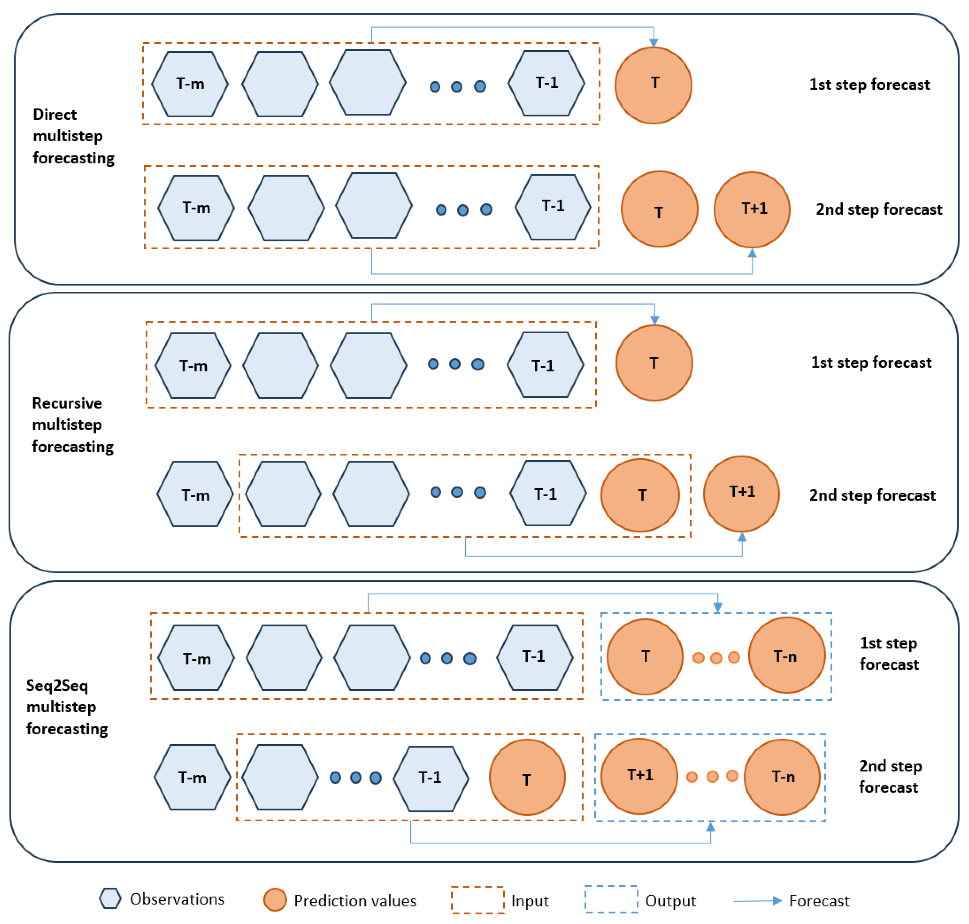
• Direct Forecasting: In this method, target values are anticipated for each subsequent step without reference to previously projected values. It is a simple strategy; however, it may suffer from the accumulation of errors [20].
• Recursive Forecasting: In this technique, the predicted values from previous steps are used as inputs to predict the values for the next step. Each predicted value serves as an input for the succeeding prediction in an iterative process. This method has the potential to better identify intertemporal dependencies [21].
• Sequence-to-Sequence Forecasting: In sequence-to-sequence (seq2seq) forecasting, a model consists of two main components: an encoder and a decoder. The decoder is trained to transform an input sequence of historical values into it into a fixed-size vector. This vector is fed into the decoder as an initial state, which focuses on different portions of the input sequence to generate the output sequence by predicting one value at a time. Transformers or RNNs are used for processing sequential data. Long-term forecasting can benefit from the use of sequence-to-sequence models since they can effectively capture complicated temporal trends [22].

ML Algorithms

In recent years, ML techniques have gained increasing popularity, with numerous studies and research papers demonstrating their superior performance compared to statistically based forecasting algorithms for time series problems [13]. The prediction methods and algorithms that we experimented with in our work can be categorized into two groups: Ensemble Decision-Tree-based models and RNNs.

Ensemble Tree-Based (ETB) models: Decision-Tree-based algorithms are non-parametric supervised learning algorithms that are used for classification and regression tasks. They feature a hierarchical, tree-like structure that represents how different input variables can be leveraged to predict a target value. This structure encompasses a root node, branches, internal nodes, and leaf nodes [23,24]. The input variables are recurrently partitioned into subsets to construct the Decision Tree, and each branch is evaluated for its prediction accuracy using conditional control statements (e.g., if–then rules) [24]. Ensemble learning techniques combine multiple simpler base algorithms to generate a predictive model with optimal performance. By combining predictions, ensemble techniques can provide more reliable and robust forecasts than single-prediction methods [25,26]. In the case of tree-based algorithms, instead of a single Decision Tree making all of the predictions, an ensemble approach is employed by creating a complete “forest” of Decision Trees. Each tree provides its prediction or “opinion” based on the data it has been trained on. The final output is determined by aggregating and considering the outputs of all trees within the forest. ETB models are known for their interpretability, versatility, prevention of overfitting, and high computational efficiency [27]. They tend to perform equally well on small and large datasets and necessitate less data preparation compared to other techniques.

Two prominent ensemble approaches are bagging (also known as Bootstrap Aggregation) and boosting (also known as Gradient Boosting). Bagging reduces the variance by averaging or combining predictions from independently trained models with equal weighting, whereas boosting reduces both the bias and variance by iteratively training models and adjusting weights, focusing on training examples that are more challenging to predict [27].

• The Random Forest (RF) algorithm is a prime example of bagging. It creates bootstrap samples that are randomly selected from the dataset and then utilizes them to grow a Decision Tree. A random subsample of the features is used in each node-splitting process. Each tree’s prediction is examined, and the choice made is recorded by the RF model. The total number of vote predictions is used to make the ultimate choice (i.e., bagging) [28]. Other examples of the bagging technique are Extra Trees (ETs) [29] and the Bagging Regressor (BR).
• The Light Gradient Boosting Machine (LGBM) is a popular Gradient Boosting method. It employs a unique approach where, before constructing a new tree, all attributes are sorted, and a fraction of the splits are examined in each iteration. These splits are conducted leaf-wise, instead of using level-wise or tree-wise splitting. The LGBM is considered a lightweight histogram-based algorithm, resulting in faster training times [30], and it is highly effective when dealing with time series data [31]. Other notable examples of boosting include the XGB [32] and Histogram-Based Gradient-Boosted Reggresor (HGBR) [33] algorithms.

Recurrent Neural Networks: RNNs are designed to retain certain elements of past observations by using a technique known as feedback. This approach allows for training to occur not just from input to output, but it also incorporates a loop inside the network to retain certain information, thereby imitating a short memory function [34]. They are proven to perform well with sequential types of data and dynamical systems modeling when compared to traditional feed-forward neural networks [34,35]. Primary examples of RNNs are Long Short-Term Memory (LSTM) and Gated Recurrent Units (GRUs).

• In contrast to conventional feed-forward neural networks, the LSTM network core components include gate and memory cells in each hidden layer and feedback connections. This structure resembles a pipeline, linking all inputs together, and highlighting those of the previous inputs that relate the most to the current inputs while diminishing the importance of those connections that are less pertinent. It is capable of handling complete data sequences (like time series, voice, or video) in addition to individual data points (i.e., image). The LSTM architecture was developed to address the issue of the vanishing gradient problem encountered by conventional RNNs when attempting to model long-term dependencies in temporal sequences. A notable variant of the LSTM is the bidirectional LSTM (biLSTM). Unlike traditional LSTMs that process sequences from past to future, biLSTMs incorporate the ability to process information in both directions [36].
• First introduced in 2014, GRUs are used as a gating technique in a RNN. Lacking an output gate, each GRU operates like an LSTM with a forget gate [37,38] but with fewer parameters. For example, in polyphonic music modeling, voice signal modeling, and natural language processing, GRUs performed better than the LSTM. Also, on smaller datasets, GRUs have been shown, on some occasions, to outperform LSTMs [39].

2.3. Related Work on Traffic Flow Predictions

Traffic management systems, empowered by advanced technologies and data-driven approaches, play a pivotal role in optimizing traffic control. The ITS infrastructure can integrate ML methods and predictive analytics to analyze real-time and historical traffic data, enabling accurate forecasting of future traffic patterns. As a result, data-driven approaches utilizing advanced forecasting models have received a lot of research attention in recent years.

To deal with a typical ITS case study, the usage of dynamic traffic statistics to accurately estimate traffic flow due to the exponential growth of traffic data, the study presented in [40] proposed a multi-step prediction model based on a Convolutional Neural Network (CNN) and bidirectional LSTM (biLSTM) model to address this problem. To extract the traffic’s time series characteristics, the biLSTM model considered the geographic features of the traffic data as the input. The experimental findings confirmed that, when compared to support vector regression and gated repeating unit models, the biLSTM model increased the prediction accuracy.

A prediction method based on the combination of Multiple Linear Regression and LSTM (MLR-LSTM) was proposed [41]. It uses both continuous and complete traffic flow data from each adjacent section’s past period, as well as incomplete traffic flow data from the target prediction section’s past period. The goal is to jointly predict changes in the target section’s traffic flow in a short amount of time.

Furthermore, to forecast the short-term traffic flow, a traffic flow prediction model that combines the XGB algorithm with wavelet decomposition and reconstruction was presented by the authors of [42]. The wavelet de-noising algorithm is first used in the training phase to gather high- and low-frequency data about the target traffic flow. Second, the threshold method is used to process the high-frequency traffic flow data. The training label is then created by reconstituting the high- and low-frequency data. Lastly, the XGB algorithm receives the de-noised target flow and uses it to train its traffic flow prediction model.

A different ML method, employed by the authors in [16], produced an accuracy of 91% and was more suited to the data format. In addition to Cell Dwell Time (CDT) data, Global Positioning System (GPS) readings could provide more accurate information regarding traffic. The goal of this work was to extract road traffic congestion levels from GPS data and traffic-related images using mobile sensors and a Decision Tree (DT) (J48/C4.5) classifier. Data from mobile sensors may be used to monitor larger traffic sectors. In actuality, the model would detect patterns in the movement of the vehicles employing SW techniques.

In another study, the authors used several RNN-LSTM architectures to forecast the taxi traffic caused by the number of tourists visiting Beijing Capital International Airport [43]. The findings of the study used three models to build an LSTM-RNN prediction model for tourist visits. LSTM regression, LSTM with SW, and sequence-to-sequence LSTM with time steps are the three LSTM models that were used. Their outcome was that, depending on the case, a different model would offer the best outcomes for both testing and training simultaneously. Regression models with the Root Mean Square Error (RMSE) produced the best training results for the prediction of tourist visits. In the meantime, the SW model yielded the best RMSE value during the testing process.

Traffic flow prediction was implemented by integrating both pollution and traffic datasets in [44]. Various ML methods were applied, revealing that the KNN exhibited the highest accuracy. To further improve the accuracy, a bagging and stacking ensemble approach was employed. The KNN bagging ensemble model outperformed other combinations, particularly excelling in handling the dataset’s nonlinear nature. The proposed ensemble approach significantly reduced error rates by 30% compared to prior studies, effectively mitigating potential overfitting caused by outliers.

Other researchers implemented a hybrid approach combining a Kernel Extreme Learning Machine (KELM) model with a Genetic Algorithm (GA) optimization to make one-step traffic flow forecasts [45]. Their model showed an improved performance over the traditional Extreme Learning Machine (ELM) and other baseline models when tested on multiple benchmark datasets. Although the size of the tested datasets was somewhat limited, their approach was able to sufficiently capture diurnal traffic flow patterns.

Given the close correlation between traffic speeds and traffic congestion, in the work of [20], an ensembling prediction model was developed to address the complexities of multi-step traffic speed predictions. The model combines two key strategies: de-trending, which separates the dataset into mean trends and residuals, and direct forecasting, which minimizes cumulative prediction errors. The study benchmarked the ensemble-based model to other models such as Support Vector Machines (SVMs), and CatBoost, and it showed a superior performance.

Additionally, alternative approaches, such as statistical and other parametric models, are often implemented to predict traffic congestion. Statistical models typically include ARIMA and its variants [46,47,48]. Other parametric methods such as fuzzy logic models [49,50]), predictive frameworks utilizing Kalman filters [51,52], and Bayesian networks [53]. In the realm of time series forecasting, such methods have been widely utilized due to their mathematical simplicity and versatility in previous years. However, their interpretability and straightforward nature often fall short of capturing the complexities of data patterns, particularly when dealing with nonlinear and long-term dependencies [54,55]. As ML techniques gain prominence, numerous studies and research papers are highlighting the limitations of statistical methods compared to state-of-the-art ML and DL algorithms across a variety of applications [34,56,57] and particularly regarding traffic prediction [58,59]. This has led to a noticeable shift towards such methods and often a hybridization approach of parametric methods and ML/DL algorithms [60,61]. Consequently, we considered experimenting with such methods by testing well-established and efficient algorithms which are currently regarded as state-of-the-art in the field.

Concerning the selected forecasting strategy, compared with the single-step method, multi-step predictions can provide future traffic conditions to allow road traffic participants to plan their routes and make decisions over a more extended time horizon. This enables adaptive decision-making as road conditions evolve. Hence, participants can adjust their plans based on changing predictions, optimizing their routes dynamically to account for real-time developments.

3. Methodology

The focus of this research was to develop an ML-based methodology for traffic congestion prediction utilizing local weather data. Our case study is based on various locations within a city environment with continuous recording of the traffic flow. Such forecasts could assist drivers with avoiding congested areas and selecting routes with better flow.

Our approach was to collect data from different sources, such as online web portals and APIs, by utilizing varying algorithms and techniques, including feature engineering and preprocessing, to predict traffic flow.

3.1. Dataset Description

Two main sources of raw data were utilized:

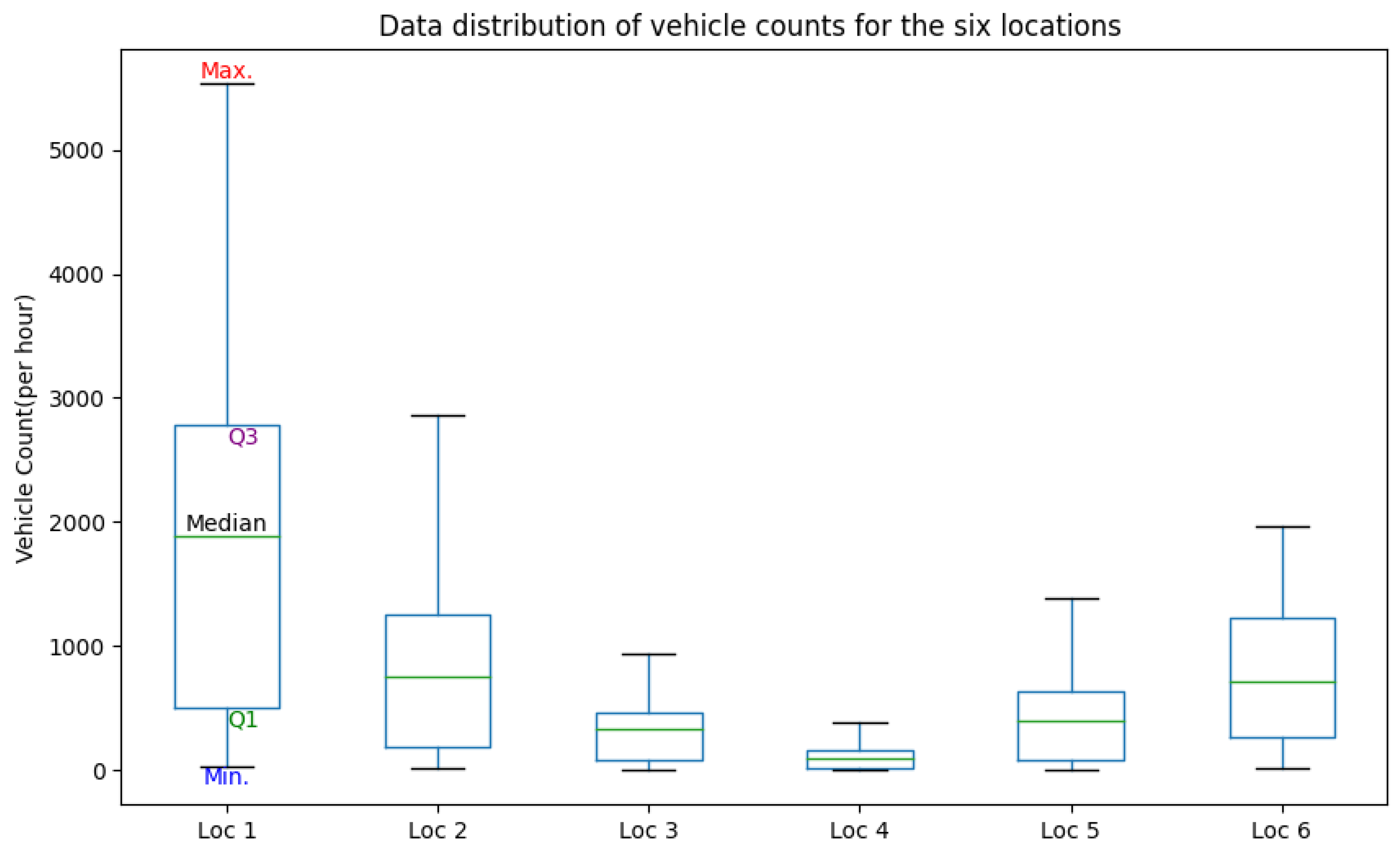
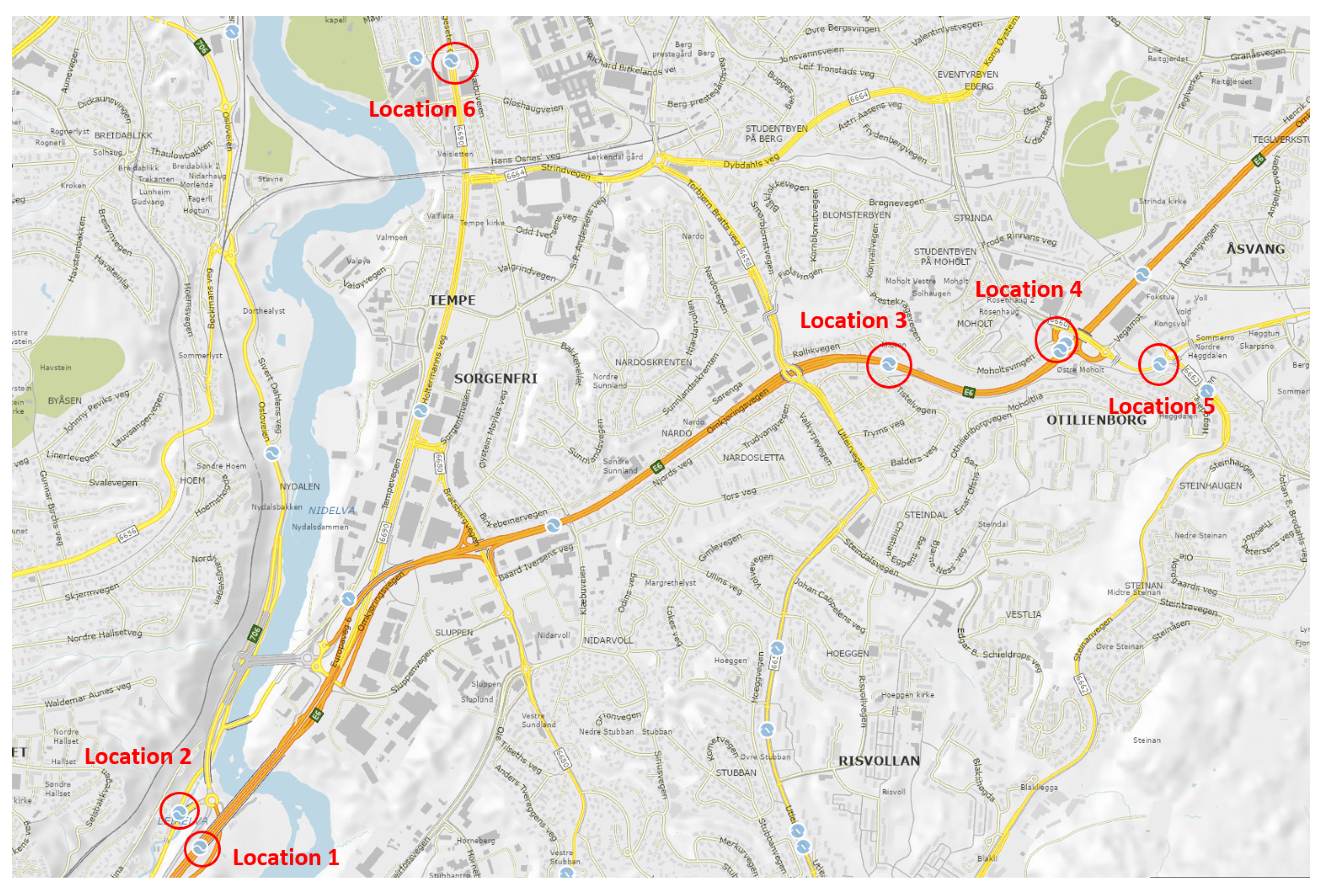
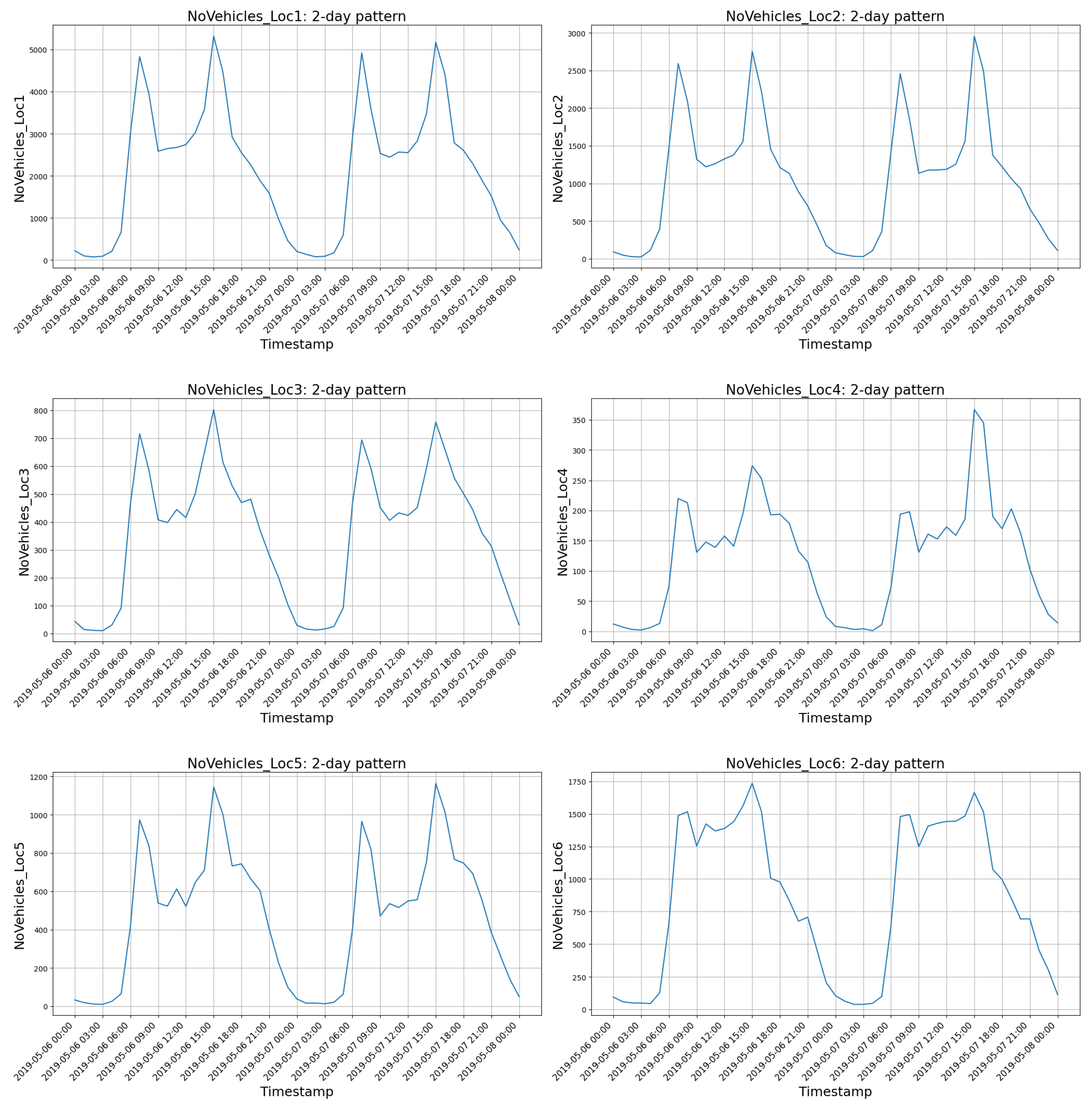
• Traffic flow data: Traffic data were collected from [62]. This web portal provides local hourly traffic flow sensor data for six traffic locations in the city of Trondheim (Figure 2). The time series data include an hourly count of vehicles shorter than 5.6 m (i.e., passenger cars) collected from December 2018 to January 2020.
• Weather condition data: Weather condition data were extracted from [63]. The data were gathered during the same period as for traffic flow data for the Trondheim area and included variables such as the relative humidity, temperature, wind speed, cloud coverage, snow depth, precipitation, and timestamp for each one hour gap.

Figure 3 presents a comprehensive summary of the descriptive statistics for traffic data collected hourly across all six locations. Location 1 stands out with the highest mean count, registering approximately 1850 vehicles passing through. A significant volume of vehicles pass through this point, as it is located before a highway bridge, essentially acting as an entry point to Trondheim. The data for Location 1 show the highest variability compared to the other locations (std. deviation of around 1400), indicating temporal reasons due to commute patterns from/to the outskirts of the city. Location 2 exhibits a lower mean vehicle count (around 830), as this location serves as a road leading to the highway. Location 4 is located on a ramp that leads vehicles to and from the same highway, thus also exhibiting lower counts. In general, Locations 3, 4, and 5 are not part of the primary route towards the city center, which may explain the lower overall count of cars.

Figure 4 depicts the daily pattern for all locations, which is characterized by a surge in the number of vehicles during the morning rush hour, with a peak typically observed at around 8:00 a.m. This peak corresponds to the typical hours when individuals are heading to work. In the evening, there is another peak at around 4:00 p.m., coinciding with the end of the workday, as people are returning to their residences. That said, it should be acknowledged that there is significant variation in the traffic flow distribution on different days of the week. Especially on weekends and holidays, there is reduced commuting towards the city center, but there can be potential spikes in recreational travel, particularly on highways leading out of the city or to recreational venues (e.g., shopping centers, stadiums, etc.).

3.2. Data Preprocessing

The first step was to merge the two datasets (traffic and weather) with the hourly timestamp parameter. The data preprocessing involved filling in any missing values. A forward/backward linear interpolation technique was employed to fill in the missing values for parameters with less than four continuous missing timestamps (four hours) and a low percentage of missing entries (less than 5%).

Normalization methods were used for the ETB and non-ETB models after accounting for the missing data. The primary method used involved scaling the data into the range of [−1, 1], based on the min/max values. This method is frequently employed in time series regression-based models.

3.3. Feature Selection and Engineering

Initially, we implemented an automated feature selection process for the weather data. We combined two well-known methods: Recursive Feature Elimination with Cross Validation (RFECV) and Sequential Forward Selection (SFS).

RFECV [64]: This is a feature selection method that fits a model (in this instance, LGBM) and eliminates the weakest feature (or features) until the desired number of features is reached. RFECV necessitates a certain number of features to be retained, but it is frequently unknown beforehand how many features are legitimate. Cross validation (CV) is used with Recursive Feature Elimination (RFE) to score various feature subsets and select the highest-scoring collection of features to determine the optimal number of features.

SFS [65,66]: Sequential feature selection is a type of greedy search algorithm that reduces an initial d-dimensional feature space to a k-dimensional feature subspace where k < d. The goal is to automatically select a subset of features that are most pertinent to the predicted target variable. In SFS, the algorithm initializes with just one of the features and tries to model the data using the given model (LGBM). Then, it selects the feature that provides the highest forecasting accuracy for the target variable.

This combined approach allowed us to identify a set of features that were particularly relevant to our analysis. Our initial list of features included a wide range of meteorological and environmental parameters. After combining the RFECV and SFS outcomes, a subset of the above features was selected for model training (“Selected” column,

Table 1. Weather data description.

Feature	Description	Unit	Selected
temp	Ambient temperature	°C	✓
feelslike	Human perceived temperature	°C	✓
dew	Dew point	°C
humidity	Relative humidity	%	✓
precip	Precipitation	mm	✓
precipprob	Precipitation chance	%
snowdepth	Depth of snow	%	✓
winddir	Direction of winds	degrees
windspeed	Speed of wind	kph	✓
sealevelpressure	Sea level pressure	mb	✓
cloudcover	Cloud coverage	%
visibility	Visibility	km	✓
solarradiation	Solar radiation	W/m2	✓
solarenergy	Solar energy	MJ/m2
UVindex	Intensity of ultraviolet radiation	-

), which was consistently informative and exhibited the strongest relationship with our target variables.

Feature engineering refers to the transformation of raw data into features to better capture relevant patterns and relationships within the data. When training a supervised ML algorithm, the creation or modification of features aims to enable better generalization of new data and increase the model’s forecasting accuracy. In our case, as we are dealing with a time series, the timestamp was divided into categorical values to generate additional seasonality features. In addition to the commonly employed temporal features such as the hour of the day, the day of the week, and the month of each load data point, certain features were synthesized based on the characteristics of our dataset, such as a feature distinguishing 3 h time intervals within the day, as commuting intensifies in the early morning hours (i.e., 06:00 to 09:00) and in the afternoon (i.e., 15:00 to 18:00), as depicted in

Table 2. Seasonality features.

Feature	Description
quarter	Corresponding to the 3 month quarter
month	Corresponding to the month of the year
hour24	Corresponding to the hour of the day
Week_day	Corresponding to the day of the week
is_weekend	Corresponding to Saturday, Sunday
off_hours	Distinguishing off-peak hours (i.e., after 17:00)
working_hours	Distinguishing peak hours (i.e., 8:00–17:00)
00 to 03, 03 to 06, …21 to 00	Distinguishing 3 h time intervals within the day

.

Overall, after combining the weather-related and seasonality features, the final features space consisted of 24 exogenous parameters to be used for training. Furthermore, the SW method was utilized to extract the previous 24 h lagged values for all selected features, as described in Section 2.2.

3.4. Forecasting Approach

We selected the direct multi-step forecasting approach with a forecasting horizon of 24 steps overall (i.e., 24 h ahead). The dataset was then divided, using a train-test split, into training and testing segments (80–20%), having nearly ten months for training and two months for testing. Overall, in our modeling approach, we sought a two-fold goal:

• To investigate the utilization of ensemble techniques such as bootstrap aggregating (bagging) and boosting, which have been extensively employed in the existing literature for road traffic flow forecasting;
• To explore the deployment of more potent Deep Learning algorithms, allowing us to conduct a comprehensive comparative analysis of their predictive performances in contrast to traditional ensemble methods.

Initially, we trained various ETB models, only for the first step ahead forecast. In total, 17 algorithms were tested. These included RF, LBGM, XGB, HGBR, ET, BR, Multilayer Perceptron (MLP) [67], Least Angle Regression CV (LarsCV) [68], Gradient-Boosted Decision Trees (GBDT) [33], LassoCV [69], LassoLarsCV, Elastic Net Regression (ENR) [70], Bayesian Ridge Regression (BRR) [71], Ridge Regression (RR) [72], Linear Regressor (LR) [73], and Huber Regressor (HR) [74]. The overall forecasting approach is illustrated in Figure 5.

Based on the evaluation metrics of the first step ahead forecast, we selected the top seven best-performing algorithms to use for the next steps. The selected algorithms were all ETB models incorporating ensembling methods: RF, LBGM, XGB, GBDT, HGBR, ET, and BR. These top-performing models were selected for further forecasting accuracy improvement through hyperparameter tuning. By utilizing the Grid Search Cross Validation (GSCV) method, which explores a predefined set of hyperparameter combinations to identify the optimal configuration that maximizes the model’s performance, we identified the optimal combination of hyperparameters for each model.

In parallel, we selected three established RNNs for time series forecasting: LSTM, biLSTM, and the GRU. To train the selected RNNs, a three-dimensional SW framework was adopted. The data were grouped into a tensor with dimensions indicating rows, time steps, and features. For the TB models, on the other hand, the traditional two-dimensional SW structure was implemented. Overall, the architecture and parameters of the RNNs are depicted in

Table 3. RNN architectural parameters.

Parameter	LSTM	biLSTM	GRU
Hidden layers	1	1	1
Units (in each hidden layer)	24	24	24
Activ. function	ReLU	ReLU	ReLU
Batch size	16	16	16
Epochs	35	35	35
Optimizer	adam	adam	adam
Dropout	0.2	0.2	0.2
SW length	24	24	24
Loss function	MAE	MAE	MAE
Early stopping (consecutive epochs)	10	10	10

.

4. Results and Evaluation

In this section, we present the findings of the experimental modeling. The statistical metrics used to evaluate models’ performances included the Mean Absolute Error (MAE), RMSE, R-squared ($R^2$), and Coefficient of the Variation of the RMSE (CVRMSE). In particular, for the first step ahead of prediction (

Table 4. First step ahead traffic flow forecasting metrics.

	Location 1				Location 2				Location 3
Model	MAE	RMSE	$R^2$ (%)	CV-RMSE	MAE	RMSE	$R^2$ (%)	CV-RMSE	MAE	RMSE	$R^2$ (%)	CV-RMSE
ET	107.89	190.68	98.16	0.105	64.74	115.00	97.64	0.130	24.69	39.45	94.76	0.134
LBGM	115.54	208.42	97.80	0.114	71.24	124.20	97.25	0.140	26.27	42.56	94.95	0.145
HGBR	117.76	211.43	97.74	0.116	70.18	122.59	97.32	0.138	26.26	42.29	94.79	0.144
GBDT	139.99	232.83	97.26	0.128	82.03	133.99	96.80	0.151	29.43	44.66	93.90	0.152
XGB	125.65	227.31	97.39	0.125	75.95	131.66	96.91	0.148	27.06	43.56	94.54	0.148
RF	112.54	208.25	97.81	0.114	68.47	123.64	97.27	0.139	25.28	41.38	94.69	0.141
BR	119.92	218.60	97.58	0.120	73.56	129.42	97.01	0.146	26.79	43.53	94.41	0.148
LSTM	210.01	354.80	93.66	0.194	184.56	315.08	92.58	0.212	38.11	62.75	93.20	0.203
biLSTM	227.91	356.84	93.59	0.195	196.22	314.99	92.59	0.212	38.99	60.25	93.73	0.195
GRU	234.79	381.81	92.66	0.208	172.40	296.89	93.41	0.200	39.68	64.99	92.71	0.210
	Location 4				Location 5				Location 6
ET	11.89	19.92	95.12	0.191	34.44	56.59	97.31	0.131	68.71	101.57	96.22	0.138
LBGM	12.39	20.24	94.96	0.194	37.51	59.43	97.04	0.137	66.75	102.95	96.12	0.140
HGBR	12.45	20.72	94.72	0.198	37.34	37.34	97.04	0.137	66.11	100.59	96.3	0.137
GBDT	13.22	21.63	94.25	0.207	40.77	63.26	96.64	0.146	79.94	114.45	95.2	0.156
XGB	13.13	21.25	94.45	0.204	38.03	59.97	96.98	0.139	66.91	100.09	96.33	0.136
RF	12.57	21.55	94.29	0.206	34.52	57.40	97.24	0.133	69.12	106.73	95.83	0.145
BR	13.60	23.09	93.44	0.221	37.50	61.33	96.84	0.142	75.03	115.20	95.14	0.157
LSTM	17.19	29.09	93.97	0.193	57.91	89.57	93.62	0.197	81.98	134.86	92.68	0.205
biLSTM	18.87	31.81	92.80	0.211	49.98	81.29	94.74	0.179	69.75	108.54	95.26	0.165
GRU	16.50	28.61	94.17	0.190	54.59	85.85	94.14	0.189	71.87	119.71	94.23	0.182

), the ETB models consistently demonstrated strong performances across the board. They exhibited low MAE and RMSE values, as well as high $R^2$ scores, indicating their ability to accurately predict traffic flow in all locations.

ET appears to be the top performer for step 1, across all locations, with LBGM and HGBR following closely. In the case of the RNNs, the performance of all tested models appears to be closely aligned, with distinctions emerging based on the location. However, they both fall behind in terms of their predictive performance compared with the ETB models, as suggested by the evaluation metrics.

Figure 6 and Figure 7 illustrate the $R^2$ and CVRMSE values of the top performing algorithms utilized in the direct multi-step ahead prediction. Regarding the direct multi-step models’ performances, we first noticed that the prediction accuracy of each model decreased with an increase in the prediction step. This result was expected as the literature indicates that multi-step prediction tends to suffer from error accumulation problems over longer prediction horizons [75]. Despite that, for all locations, the ETB models showed improved predictions for all time steps ahead, in contrast with the RNNs, which fell behind with very few exceptions.

Focusing on the RNNs, they generally demonstrated higher variability between steps. Considering all future steps, LSTM and GRU slightly outperformed biLSTM, on average; hence, we focus on them. In most traffic locations, during the first steps (i.e., 1–8), they had similar performances, while toward the last steps (i.e., 20–24), GRU seemed to improve its performance over the LSTM. The developed RNNs failed to achieve an improved performance over the ETB models in terms of reflecting the periodicity of the traffic flow. Also, they required longer training times since they involved more expensive computations. As the literature suggests, RNNs typically require large amounts of data with added complexities in their pattern to maximize their prediction accuracy. This may explain the deterioration in their forecasting performance, as our dataset is limited to only a year in an hourly resolution.

Focusing on the performance of the ETB models, we aim to present a more detailed description of their performances, as further described in

Table 5. Frequency count for the top seven performing models in each of the first four steps and in all 24 steps.

	RF	ET	HGBR	LGBM	XGB	GBDT	BR
First 4 Steps
Location 1	4	4	4	3	3	2	0
Location 2	4	4	4	4	3	1	0
Location 3	4	4	4	4	3	1	0
Location 4	3	4	4	4	3	0	2
Location 5	4	4	4	4	2	0	2
Location 6	4	4	4	4	4	0	0
All 24 Steps
Location 1	24	23	22	21	17	8	5
Location 2	22	24	24	24	20	5	1
Location 3	24	12	24	24	15	8	13
Location 4	19	24	24	24	16	12	1
Location 5	19	24	24	24	13	10	6
Location 6	24	19	23	23	22	0	9

. For each time step ahead, we determined the top seven performing models based on their $R^2$ performances. First, we assessed the first four steps, as the performances of the models were very similar in terms of metrics, as depicted by Figure 6 and Figure 7. Then, we assessed all 24 steps. Specifically, the values represent how many times a model was present in the top seven performing algorithms for each forecasting step. As an example, for Location 1, RF, ET, HGBR, LGBM, XGB, GBDT, and BR were present 24, 23, 22, 21, 17, 8, and 5 times, respectively, in the top seven performing algorithms. Notably, RF consistently demonstrated a high level of accuracy for all 24 forecasting steps for Location 1 (particularly steps 8–14), Location 3, and Location 6 (particularly steps 10–24). Considering the performance across all locations, HGBR and LGBM stand out as the models with the best overall performances. They consistently demonstrated high accuracy throughout the entire 24 h forecasting period, making them the primary choices. ET and RF showed high levels of accuracy, but not across all locations. ET was the best-performing algorithm for Location 2 (especially after the first seven steps) and Location 4 (across all steps). RF prevailed over other algorithms in Location 3 after the first few steps. XGB fell slightly behind, as apart from the last steps for Location 1 (18–24), its performance fell significantly, especially in Locations 3, 4, and 5. GBDT and BR emerged as the worst-performing algorithms overall.

Compared to the highly relevant work by [45], their approach employed a more automated hyperparameter tuning method (GA) that required fewer computational resources, particularly when applied to diverse datasets. It is worth noting, however, that their approach is limited to a one-step-ahead forecasting strategy, whereas our model predicts 24 steps into the future. Hence, when focusing on the one-step-ahead evaluation of the performance metrics of our approach, the top-performing models of our approach for each location had similar performance levels. However, it is essential to consider that our model was trained and tested on more chronically extensive datasets (spanning one year) compared to the few weeks utilized by the GA-KELM model. This extended dataset encompasses variations attributed to seasonality effects, including weather changes, vacation periods, and annual events. Such factors may potentially contribute to a more comprehensive evaluation of our model’s robustness in real-world scenarios for longer periods of time.

5. Conclusions

Through the examination of data derived from IoT sensors and historical traffic patterns, ML models possess the ability to predict the timing and location of congestion. Such models can be integrated into a broader Intelligent Transportation System (ITS) infrastructure by leveraging data to notify motorists, suggest alternate routes, optimize signal timings, and enhance the overall traffic management.

The objective of this work was to improve the accuracy of time series forecasting for multi-location, multi-step-ahead predictions of traffic flow in an urban setting. Our work encompassed a thorough evaluation and comparison of several ML and DL models in six locations. Traffic flow predictions are also impacted by exogenous variables other than prior traffic flow data. Weather, holidays, and other contextual circumstances may all have substantial influences on traffic flow variations. Hence, the predictive models developed were enhanced by feature selection and engineering methods regarding temporal and weather data. The paper proposes a unique strategy to provide an accurate step-by-step prediction framework through the implementation of interpretable models. The novel aspect of this work is attributed to a selection approach that employs the best-performing predictive algorithms at each forecasting step, which can be compared to existing state-of-the-art approaches in the area.

The comparative analyses of the prediction results illustrated that, overall, the DL implementations fall behind compared to traditional shallow learning models, such as Decision Tree Ensemble regressors. Focusing on the latter, depending on the traffic location and the timestep ahead, a different algorithm can be deployed. In particular, for longer forecasting horizons, ET and RF outperform other algorithms in almost all traffic locations. Although their prediction accuracy decreases as we progress towards the latter steps, even in the 24th step, the evaluation metrics show that the models achieve a high level of accuracy, especially when compared to other closely relevant research studies (such as [44]). That said, considering the overall performance over all locations and future steps in the forecasting horizon, HGBR and LGBM are, on average, the most reliable models, especially for the first few steps.

5.1. Limitations

The most potent limitation of this study pertains to the efficacy of the algorithms, which is intricately linked to the statistical characteristics of the case study dataset. Data gathered from other locations and for different time intervals may exhibit diverse statistical features, resulting in disparate findings. However, our approach deploys a varying range of models each time, selecting the best performer. Therefore, it enables more adaptive behavior in terms of the predictive performance and is capable of capturing the diversification and randomness of new data.

Moreover, the granularity and size of the data are important impediments to the development of a predictive framework with increased generalization. The limited size of the training data may have negatively affected the performance of DL models (e.g., LSTM), which, according to scientific studies, often demand high volumes of data to reach higher levels of accuracy. Additional parameter tuning and training could improve the results for the implemented RNNs. Nevertheless, managing a large amount of data can be challenging and requires careful balancing. High-volume datasets can appear as complex information networks and aid in model training for supervised or semi-supervised learning, but they may also generate time and space complexity issues.

5.2. Future Work

Concerning future work, experimenting with more diverse and extensive datasets from other urban traffic locations and sensors can help to ensure robustness and increased generalization in our approach. In addition, hidden links between traffic flows in various areas have been discovered. Investigating the impacts of these external elements on traffic flow prediction, especially their hidden characteristics, could greatly improve the accuracy of future forecasts. In a more technical context, regarding the future expansion of this work, potential areas of further research to consider are the following:

• Introducing closely related spatial features to the developed models, for example, public bus arrivals and departures or ride-hailing orders in the area.
• The performance of experimental modeling utilizing larger and more diverse training datasets with added complexities. With the added data, the behavior of the implemented RNNs should be closely examined.
• Additional DL techniques could be explored, such as CNNs combined with a RNN implementation, possibly under a CNN-LSTM configuration. The public availability of comprehensive and extensive traffic flow datasets is typically limited. However, there are approaches within the field of Transfer Learning (TL) that have been developed to solve new but comparable problems by utilizing prior knowledge. Integrating existing knowledge when training such DL models allows a reduction in the amount of required training data and leads to better learning rates [76]. Examples of such methods can be found in [77,78], where the outputs of physics-based models were utilized as soft constraints to penalize or regulate data-driven implementations, and in [79], where a fusion of prior knowledge network was developed using self-similarity properties of network traffic data.
• Integration of this traffic forecasting approach as a component in another expanded forecasting framework. For example, a localized EV charging demand forecasting framework could be utilized to predict the short-term EV charging load demand.

References

1. United Nations. World Urbanization Prospects: The 2018 Revision; Technical Report; UN: New York, NY, USA, 2019. [Google Scholar]
2. Zhang, K.; Batterman, S. Air pollution and health risks due to vehicle traffic. Sci. Total Environ. 2013, 450–451, 307–316. [Google Scholar] [CrossRef]
3. Gakis, E.; Kehagias, D.; Tzovaras, D. Mining Traffic Data for Road Incidents Detection. In Proceedings of the 2014 IEEE 17th International Conference on Intelligent Transportation Systems (ITSC), Qingdao, China, 8–11 October 2014. [Google Scholar]
4. Shokri, D.; Larouche, C.; Homayouni, S. A Comparative Analysis of Multi-Label Deep Learning Classifiers for Real-Time Vehicle Detection to Support Intelligent Transportation Systems. Smart Cities 2023, 6, 2982–3004. [Google Scholar] [CrossRef]
5. Kontses, A.; Triantafyllopoulos, G.; Ntziachristos, L.; Samaras, Z. Particle number (PN) emissions from gasoline, diesel, LPG, CNG and hybrid-electric light-duty vehicles under real-world driving conditions. Atmos. Environ. 2020, 222, 117126. [Google Scholar] [CrossRef]
6. European Commission. Impact of Driving Conditions and Driving Behaviour—ULEV. 2023. Available online: https://wikis.ec.europa.eu/display/ULEV/Impact+of+driving+conditions+and+driving+behaviour (accessed on 31 October 2023).
7. Regragui, Y.; Moussa, N. A real-time path planning for reducing vehicles traveling time in cooperative-intelligent transportation systems. Simul. Model. Pract. Theory 2023, 123, 102710. [Google Scholar] [CrossRef]
8. MACIOSZEK, E. Analysis of the volume of passengers and cargo in rail and road transport in Poland in 2009–2019. Sci. J. Silesian Univ. Technol. Ser. Transp. 2021, 113, 133–143. [Google Scholar] [CrossRef]
9. Oladimeji, D.; Gupta, K.; Kose, N.A.; Gundogan, K.; Ge, L.; Liang, F. Smart Transportation: An Overview of Technologies and Applications. Sensors 2023, 23, 3880. [Google Scholar] [CrossRef]
10. Razali, N.A.M.; Shamsaimon, N.; Ishak, K.K.; Ramli, S.; Amran, M.F.M.; Sukardi, S. Gap, techniques and evaluation: Traffic flow prediction using machine learning and deep learning. J. Big Data 2021, 8, 152. [Google Scholar] [CrossRef]
11. Mystakidis, A.; Stasinos, N.; Kousis, A.; Sarlis, V.; Koukaras, P.; Rousidis, D.; Kotsiopoulos, I.; Tjortjis, C. Predicting Covid-19 ICU Needs Using Deep Learning, XGBoost and Random Forest Regression with the Sliding Window Technique. In Proceedings of the IEEE Smart Cities, Virtual, 17–23 March 2021; pp. 1–6. [Google Scholar]
12. Mystakidis, A.; Ntozi, E.; Afentoulis, K.; Koukaras, P.; Gkaidatzis, P.; Ioannidis, D.; Tjortjis, C.; Tzovaras, D. Energy generation forecasting: Elevating performance with machine and deep learning. Computing 2023, 105, 1623–1645. [Google Scholar] [CrossRef]
13. Tsalikidis, N.; Mystakidis, A.; Tjortjis, C.; Koukaras, P.; Ioannidis, D. Energy load forecasting: One-step ahead hybrid model utilizing ensembling. Computing 2023, 106, 241–273. [Google Scholar] [CrossRef]
14. Koukaras, P.; Tjortjis, C.; Gkaidatzis, P.; Bezas, N.; Ioannidis, D.; Tzovaras, D. An interdisciplinary approach on efficient virtual microgrid to virtual microgrid energy balancing incorporating data preprocessing techniques. Computing 2022, 104, 209–250. [Google Scholar] [CrossRef]
15. Olshausen, B.A.; Field, D.J. Emergence of simple-cell receptive field properties by learning a sparse code for natural images. Nature 1996, 381, 607–609. [Google Scholar] [CrossRef] [PubMed]
16. Thianniwet, T.; Phosaard, S.; Pattara-atikom, W. Classification of Road Traffic Congestion Levels from GPS Data using a Decision Tree Algorithm and Sliding Windows. Lecture Notes in Engineering and Computer Science. In Proceedings of the World Congress on Engineering 2009 Vol I WCE 2009, London, UK, 1–3 July 2009. [Google Scholar]
17. Heidari, A.; Navimipour, N.J.; Unal, M. Applications of ML/DL in the management of smart cities and societies based on new trends in information technologies: A systematic literature review. Sustain. Cities Soc. 2022, 85, 104089. [Google Scholar] [CrossRef]
18. Adel, A. Unlocking the Future: Fostering Human–Machine Collaboration and Driving Intelligent Automation through Industry 5.0 in Smart Cities. Smart Cities 2023, 6, 2742–2782. [Google Scholar] [CrossRef]
19. Lee, C.H.; Lin, C.R.; Chen, M.S. Sliding-Window Filtering: An Efficient Algorithm for Incremental Mining. In Proceedings of the International Conference on Information and Knowledge Management, Atlanta, GA, USA, 5–10 October 2001; pp. 263–270. [Google Scholar] [CrossRef]
20. Feng, B.; Xu, J.; Zhang, Y.; Lin, Y. Multi-step traffic speed prediction based on ensemble learning on an urban road network. Appl. Sci. 2021, 11, 4423. [Google Scholar] [CrossRef]
21. Xue, P.; Jiang, Y.; Zhou, Z.; Chen, X.; Fang, X.; Liu, J. Multi-step ahead forecasting of heat load in district heating systems using machine learning algorithms. Energy 2019, 188, 116085. [Google Scholar] [CrossRef]
22. Mariet, Z.; Kuznetsov, V. Foundations of Sequence-to-Sequence Modeling for Time Series. In Proceedings of the Twenty-Second International Conference on Artificial Intelligence and Statistics, PMLR, Okinawa, Japan, 16–18 April 2019; Volume 89, pp. 408–417. [Google Scholar]
23. Song, Y.Y.; Lu, Y. Decision tree methods: Applications for classification and prediction. Shanghai Arch. Psychiatry 2015, 27, 130–135. [Google Scholar] [CrossRef] [PubMed]
24. Breiman, L.; Friedman, J.H.; Olshen, R.A.; Stone, C.J. Classification and Regression Trees; Chapman & Hall: Boca Raton, FL, USA, 1984. [Google Scholar]
25. Ruiz-Abellón, M.D.C.; Gabaldón, A.; Guillamón, A. Load forecasting for a campus university using ensemble methods based on regression trees. Energies 2018, 11, 2038. [Google Scholar] [CrossRef]
26. Natras, R.; Soja, B.; Schmidt, M. Ensemble Machine Learning of Random Forest, AdaBoost and XGBoost for Vertical Total Electron Content Forecasting. Remote Sens. 2022, 14, 3547. [Google Scholar] [CrossRef]
27. Omer, Z.M.; Shareef, H. Comparison of decision tree based ensemble methods for prediction of photovoltaic maximum current. Energy Convers. Manag. 2022, 16, 100333. [Google Scholar] [CrossRef]
28. Breiman, L. Random Forests. Mach. Learn. 2001, 45, 5–32. [Google Scholar] [CrossRef]
29. Geurts, P.; Ernst, D.; Wehenkel, L. Extremely randomized trees. Mach. Learn. 2006, 63, 3–42. [Google Scholar] [CrossRef]
30. Ju, Y.; Sun, G.; Chen, Q.; Zhang, M.; Zhu, H.; Rehman, M.U. A model combining Convolutional Neural Network and LightGBM algorithm for ultra-short-term wind power forecasting. IEEE Access 2019, 7, 28309–28318. [Google Scholar] [CrossRef]
31. Makridakis, S.; Spiliotis, E.; Assimakopoulos, V. M5 accuracy competition: Results, findings, and conclusions. Int. J. Forecast. 2022, 38, 1346–1364. [Google Scholar] [CrossRef]
32. Chen, T.; Guestrin, C. XGBoost: A scalable tree boosting system. In Proceedings of the ACM SIGKDD International Conference on Knowledge Discovery and Data Mining, San Francisco, CA, USA, 13–17 August 2016; pp. 785–794. [Google Scholar] [CrossRef]
33. Friedman, J.H. Greedy function approximation: A gradient boosting machine. Ann. Stat. 2001, 29, 1189–1232. [Google Scholar] [CrossRef]
34. Siami-Namini, S.; Tavakoli, N.; Namin, A.S. The Performance of LSTM and BiLSTM in Forecasting Time Series. In Proceedings of the 2019 IEEE International Conference on Big Data (Big Data), Los Angeles, CA, USA, 9–12 December 2019. [Google Scholar]
35. Omlin, C.; Thornber, K.; Giles, C. Fuzzy finite-state automata can be deterministically encoded into recurrent neural networks. IEEE Trans. Fuzzy Syst. 1998, 6, 76–89. [Google Scholar] [CrossRef]
36. Hochreiter, S.J.; Schmidhuber, J. Long short-term memory. Neural Computation 1997, 9, 1735–1780. [Google Scholar] [CrossRef]
37. Gers, F.; Schmidhuber, J.; Cummins, F. Learning to forget: Continual prediction with LSTM. Neural Comput. 1999, 12, 2451–2471. [Google Scholar] [CrossRef] [PubMed]
38. Cho, K.; van Merrienboer, B.; Bahdanau, D.; Bengio, Y. On the Properties of Neural Machine Translation: Encoder-Decoder Approaches. arxiv 1409. [Google Scholar]
39. Gruber, N.; Jockisch, A. Are GRU Cells More Specific and LSTM Cells More Sensitive in Motive Classification of Text? Front. Artif. Intell. 2020, 3, 00040. [Google Scholar] [CrossRef]
40. Zhuang, W.; Cao, Y. Short-Term Traffic Flow Prediction Based on CNN-BILSTM with Multicomponent Information. Appl. Sci. 2022, 12, 8714. [Google Scholar] [CrossRef]
41. Shi, R.; Du, L. Multi-Section Traffic Flow Prediction Based on MLR-LSTM Neural Network. Sensors 2022, 22, 7517. [Google Scholar] [CrossRef] [PubMed]
42. Dong, X.; Lei, T.; Jin, S.; Hou, Z. Short-Term Traffic Flow Prediction Based on XGBoost. In Proceedings of the 2018 IEEE 7th Data Driven Control and Learning Systems Conference (DDCLS), Enshi, China, 25–27 May 2018; pp. 854–859. [Google Scholar] [CrossRef]
43. Rizal, A.A.; Soraya, S.; Tajuddin, M. Sequence to sequence analysis with long short term memory for tourist arrivals prediction. J. Phys. Conf. Ser. 2019, 1211, 012024. [Google Scholar] [CrossRef]
44. Khan, N.U.; Shah, M.A.; Maple, C.; Ahmed, E.; Asghar, N. Traffic Flow Prediction: An Intelligent Scheme for Forecasting Traffic Flow Using Air Pollution Data in Smart Cities with Bagging Ensemble. Sustainability 2022, 14, 4164. [Google Scholar] [CrossRef]
45. Chai, W.; Zheng, Y.; Tian, L.; Qin, J.; Zhou, T. GA-KELM: Genetic-Algorithm-Improved Kernel Extreme Learning Machine for Traffic Flow Forecasting. Mathematics 2023, 11, 3574. [Google Scholar] [CrossRef]
46. Billings, D.; Yang, J.S. Application of the ARIMA Models to Urban Roadway Travel Time Prediction—A Case Study. In Proceedings of the 2006 IEEE International Conference on Systems, Man and Cybernetics, Taipei, Taiwan, 8–11 October 2006; Volume 3, pp. 2529–2534. [Google Scholar] [CrossRef]
47. Williams, B.M.; Hoel, L.A. Modeling and Forecasting Vehicular Traffic Flow as a Seasonal ARIMA Process: Theoretical Basis and Empirical Results. J. Transp. Eng. 2003, 129, 664–672. [Google Scholar] [CrossRef]
48. Van Der Voort, M.; Dougherty, M.; Watson, S. Combining kohonen maps with arima time series models to forecast traffic flow. Transp. Res. Part C Emerg. Technol. 1996, 4, 307–318. [Google Scholar] [CrossRef]
49. Lu, J.; Cao, L. Congestion evaluation from traffic flow information based on fuzzy logic. In Proceedings of the 2003 IEEE International Conference on Intelligent Transportation Systems, Shanghai, China, 12–15 October 2003; pp. 50–53. [Google Scholar] [CrossRef]
50. Krause, B.; von Altrock, C.; Pozybill, M. Intelligent highway by fuzzy logic: Congestion detection and traffic control on multi-lane roads with variable road signs. In Proceedings of the IEEE 5th International Fuzzy Systems, New Orleans, LA, USA, 11 September 1996; Volume 3, pp. 1832–1837. [Google Scholar]
51. Guo, J.; Huang, W.; Williams, B.M. Adaptive Kalman filter approach for stochastic short-term traffic flow rate prediction and uncertainty quantification. Transp. Res. Part C Emerg. Technol. 2014, 43, 50–64. [Google Scholar] [CrossRef]
52. Lu, C.C.; Zhou, X.S. Short-Term Highway Traffic State Prediction Using Structural State Space Models. J. Intell. Transp. Syst. 2014, 18, 309–322. [Google Scholar] [CrossRef]
53. Ghosh, B.; Basu, B.; O’Mahony, M. Bayesian Time-Series Model for Short-Term Traffic Flow Forecasting. J. Transp. Eng.—ASCE 2007, 133, 180–189. [Google Scholar] [CrossRef]
54. Yang, X.; Zou, Y.; Tang, J.; Liang, J.; Ijaz, M. Evaluation of Short-Term Freeway Speed Prediction Based on Periodic Analysis Using Statistical Models and Machine Learning Models. J. Adv. Transp. 2020, 2020, 9628957. [Google Scholar] [CrossRef]
55. Kohzadi, N.; Boyd, M.S.; Kermanshahi, B.; Kaastra, I. A comparison of artificial neural network and time series models for forecasting commodity prices. Neurocomputing 1996, 10, 169–181. [Google Scholar] [CrossRef]
56. Kontopoulou, V.I.; Panagopoulos, A.D.; Kakkos, I.; Matsopoulos, G.K. A Review of ARIMA vs. Machine Learning Approaches for Time Series Forecasting in Data Driven Networks. Future Internet 2023, 15, 255. [Google Scholar] [CrossRef]
57. Menculini, L.; Marini, A.; Proietti, M.; Garinei, A.; Bozza, A.; Moretti, C.; Marconi, M. Comparing Prophet and Deep Learning to ARIMA in Forecasting Wholesale Food Prices. Forecasting 2021, 3, 644–662. [Google Scholar] [CrossRef]
58. Shaygan, M.; Meese, C.; Li, W.; Zhao, X.G.; Nejad, M. Traffic prediction using artificial intelligence: Review of recent advances and emerging opportunities. Transp. Res. Part C Emerg. Technol. 2022, 145, 103921. [Google Scholar] [CrossRef]
59. Medina-Salgado, B.; Sánchez-DelaCruz, E.; Pozos-Parra, P.; Sierra, J.E. Urban traffic flow prediction techniques: A review. Sustain. Comput. Inform. Syst. 2022, 35, 100739. [Google Scholar] [CrossRef]
60. Zheng, W.; Lee, D.H.; Shi, Q. Short-Term Freeway Traffic Flow Prediction: Bayesian Combined Neural Network Approach. J. Transp. Eng. 2006, 132, 114–121. [Google Scholar] [CrossRef]
61. Tang, J.; Wang, H.; Wang, Y.; Liu, X.C.; Liu, F. Hybrid Prediction Approach Based on Weekly Similarities of Traffic Flow for Different Temporal Scales. Transp. Res. Rec. J. Transp. Res. Board 2014, 2443, 21–31. [Google Scholar] [CrossRef]
62. Norwegian Public Roads Administration, Trafikkdata. Available online: https://trafikkdata.atlas.vegvesen.no (accessed on 1 September 2023).
63. Weather Data & Weather API-Visual Crossing. Available online: https://www.visualcrossing.com/ (accessed on 1 September 2023).
64. Guyon, I.; Weston, J.; Barnhill, S.; Vapnik, V. Gene Selection for Cancer Classification Using Support Vector Machines. Mach. Learn. 2002, 46, 389–422. [Google Scholar] [CrossRef]
65. Ferri, F.; Pudil, P.; Hatef, M.; Kittler, J. Comparative study of techniques for large-scale feature selection. In Machine Intelligence and Pattern Recognition; North-Holland: Amsterdam, The Netherlands, 1994; Volume 16, pp. 403–413. [Google Scholar]
66. Shafiee, S.; Lied, L.M.; Burud, I.; Dieseth, J.A.; Alsheikh, M.; Lillemo, M. Sequential forward selection and support vector regression in comparison to LASSO regression for spring wheat yield prediction based on UAV imagery. Comput. Electron. Agric. 2021, 183, 106036. [Google Scholar] [CrossRef]
67. Murtagh, F. Multilayer perceptrons for classification and regression. Neurocomputing 1991, 2, 183–197. [Google Scholar] [CrossRef]
68. Efron, B.; Hastie, T.; Johnstone, I.; Tibshirani, R. Least angle regression. Ann. Stat. 2004, 32, 407–499. [Google Scholar] [CrossRef]
69. Tibshirani, R. Regression shrinkage and selection via the lasso. J. R. Stat. Soc. Ser. B (Methodol.) 1996, 58, 267–288. [Google Scholar] [CrossRef]
70. Zou, H.; Hastie, T. Regularization and variable selection via the elastic net. J. R. Stat. Soc. Ser. B (Stat. Methodol.) 2005, 67, 301–320. [Google Scholar] [CrossRef]
71. MacKay, D.J.C. Bayesian interpolation. Neural Comput. 1992, 4, 415–447. [Google Scholar] [CrossRef]
72. Hoerl, A.E.; Kennard, R.W. Ridge regression: Biased estimation for nonorthogonal problems. Technometrics 1970, 12, 55–67. [Google Scholar] [CrossRef]
73. Seber, G.A.F.; Lee, A.J. Linear Regression Analysis; John Wiley & Sons: Hoboken, NJ, USA, 2012. [Google Scholar]
74. Huber, P.J. Robust estimation of a location parameter. Ann. Math. Stat. 1964, 35, 73–101. [Google Scholar] [CrossRef]
75. Cheng, H.; Tan, P.N.; Gao, J.; Scripps, J. Multistep-Ahead Time Series Prediction. In Advances in Knowledge Discovery and Data Mining; Ng, W.K., Kitsuregawa, M., Li, J., Chang, K., Eds.; Springer: Berlin/Heidelberg, Germany, 2006; pp. 765–774. [Google Scholar] [CrossRef]
76. Manibardo, E.L.; Laña, I.; Del Ser, J. Transfer Learning and Online Learning for Traffic Forecasting under Different Data Availability Conditions: Alternatives and Pitfalls. In Proceedings of the 2020 IEEE 23rd International Conference on Intelligent Transportation Systems (ITSC), Rhodes, Greece, 20–23 September 2020; pp. 1–6. [Google Scholar] [CrossRef]
77. Zhang, J.; Zhao, Y.; Shone, F.; Li, Z.; Frangi, A.F.; Xie, S.Q.; Zhang, Z.Q. Physics-Informed Deep Learning for Musculoskeletal Modeling: Predicting Muscle Forces and Joint Kinematics From Surface EMG. IEEE Trans. Neural Syst. Rehabil. Eng. 2023, 31, 484–493. [Google Scholar] [CrossRef]
78. Zhang, J.; Zhao, Y.; Bao, T.; Li, Z.; Qian, K.; Frangi, A.F.; Xie, S.; Zhang, Z.L. Boosting Personalized Musculoskeletal Modeling with Physics-Informed Knowledge Transfer. IEEE Trans. Instrum. Meas. 2022, 72, 1–11. [Google Scholar]
79. Pan, C.; Wang, Y.; Shi, H.; Shi, J.; Cai, R. Network Traffic Prediction Incorporating Prior Knowledge for an Intelligent Network. Sensors 2022, 22, 2674. [Google Scholar] [CrossRef]
Figure 1. Three main strategies of multi-step forecasting.
Smartcities 07 00010 g001
Figure 2. Locations of measured traffic flow data in the city of Trondheim.
Smartcities 07 00010 g002
Figure 3. Descriptive statistics for hourly measured traffic data.
Smartcities 07 00010 g003
Figure 4. Two day vehicle count pattern for all traffic locations.
Smartcities 07 00010 g004
Figure 5. Overview of the forecasting approach.
Smartcities 07 00010 g005
Figure 6. Direct multi-step forecasting R 2 comparison.
Smartcities 07 00010 g006
Figure 7. Direct multi-step forecasting CVRMSE comparison.
Smartcities 07 00010 g007