Abstract
In smart city contexts, traditional methods for semantic segmentation are affected by adverse conditions, such as rain, fog, or darkness. One challenge is the limited availability of semantic segmentation datasets, specifically for autonomous driving in adverse conditions, and the high cost of labeling such datasets. To address this problem, unsupervised domain adaptation (UDA) is commonly employed. In UDA, the source domain contains data from good weather conditions, while the target domain contains data from adverse weather conditions. The Adverse Conditions Dataset with Correspondences (ACDC) provides reference images taken at different times but in the same location, which can serve as an intermediate domain, offering additional semantic information. In this study, we introduce a method that leverages both the intermediate domain and frequency information to improve semantic segmentation in smart city environments. Specifically, we extract the region with the largest difference in standard deviation and entropy values from the reference image as the intermediate domain. Secondly, we introduce the Fourier Exponential Decreasing Sampling (FEDS) algorithm to facilitate more reasonable learning of frequency domain information. Finally, we design an efficient decoder network that outperforms the DAFormer network by reducing network parameters by 28.00%. When compared to the DAFormer work, our proposed approach demonstrates significant performance improvements, increasing by 6.77%, 5.34%, 6.36%, and 5.93% in mean Intersection over Union (mIoU) for Cityscapes to ACDC night, foggy, rainy, and snowy, respectively.
1. Introduction
1.1. Semantic Segmentation of Autonomous Driving
With the continuous progress of image processing technology [1,2,3,4,5], autonomous driving technology is also developing rapidly in smart cities [6,7,8]. Enabling autonomous driving is a popular topic to better understand the semantic scenes of the real world [9,10,11,12], and semantic segmentation technology is the core technology in the field of autonomous driving. The semantic segmentation task of autonomous driving is to classify each pixel into the image semantically, so that different types of objects can be distinguished in the image. The semantic segmentation result is to divide the region of visual interest, which provides favorable guidance for subsequent image analysis and visual understanding. Autonomous driving systems need to recognize objects such as cars, traffic lights, pedestrians, bicycles, trees, lane lines, etc. The varying sizes of these objects, along with potential occlusions, introduce challenges to the semantic segmentation task [13,14]. Referring to Figure 1, which corresponds to the Cityscapes [15] dataset, captured under favorable weather conditions during daylight, it is evident that distinct colors are utilized to denote buildings, sky, trees, sidewalks, and other objects. The objective of the algorithmic model is to identify various objects. In practical scenarios, the model is trained on autonomous driving data collected under optimal daytime conditions. Consequently, the model exhibits commendable recognition efficacy under similar conditions. However, its recognition accuracy significantly diminishes when confronted with adverse weather conditions, such as low-light settings and fog [16]. This discrepancy is attributed to incongruities in data distribution between images from dissimilar weather scenarios, thereby resulting in a domain gap between them. Assuming the daytime, favorable weather scenes constitute the source domain, and adverse weather scenes represent the target domain. It becomes apparent that directly applying a model trained on source domain data to the target domain dataset yields suboptimal results. Thus, a noteworthy avenue of exploration pertains to the mitigation of the domain gap between the source and target domains.
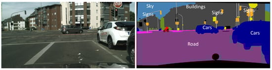
Figure 1.
The Cityscapes dataset for autonomous driving semantic segmentation. Distinct regions are delineated by varying colors, each signifying unique object semantic information.
To augment the recognition capabilities of autonomous driving systems, a continuous influx of advanced visual image sensors has surfaced. Nevertheless, these sensors remain susceptible to outdoor weather, lighting conditions, sensor noise, and other influential factors. As a result, achieving precise semantic segmentation within autonomous driving scenes continues to present a formidable challenge. It is widely recognized that deep learning has demonstrated remarkable excellence within the realm of semantic segmentation [17,18,19]. Nonetheless, it necessitates a substantial volume of labeled data, and the manual collection and labeling of datasets for autonomous driving incur excessive costs. These methodologies entail leveraging training data as the source domain and test data as the target domain, progressively mitigating the distribution disparity between the two domains through algorithmic interventions. Currently, most of the UDA semantic segmentation methods are primarily designed for tasks like fog or rain removal individually. In 2022, Hoyer et al. introduced a domain adaptation algorithm for semantic segmentation [20]. They used the GTA dataset [21], derived from gaming scenes, as the source domain for training. Subsequently, the Cityscape dataset was employed as the target domain for testing, as illustrated in Figure 2. The approach demonstrated exceptional performance.
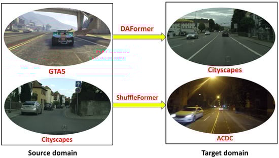
Figure 2.
In the DAFormer work, the GTA5 dataset is employed as the source domain, while the Cityscapes dataset is the target domain. Our approach involves utilizing the Cityscapes dataset as the source domain and the ACDC dataset as the target domain and crafting the specialized ShuffleFormer network tailored for autonomous driving scenarios.
1.2. Motivations
The DAFormer work demonstrates effectiveness in domain adaptation for semantic segmentation. Furthermore, its theoretical efficacy extends to the application of this method in challenging adverse weather conditions. In this paper, we enhance the DAFormer work by utilizing the Cityscapes dataset under favorable daytime conditions as the source domain and employing the ACDC dataset [22] under challenging severe weather conditions as the target domain. In recent years, numerous autonomous driving datasets [22,23,24] have incorporated supplementary reference images captured within the same scene as the target domain. Utilizing the GPS positioning information of the vehicle, one can access the reference images of the target domain captured at different times but in the same location under favorable daytime weather conditions. These reference images can complement the semantic information of the target domain. To leverage their potential, we introduce intermediary domains, depicted in Figure 3, employing these reference images to bolster the discernment of the model in the target domain. Functioning as intermediary domains, these reference images synergistically offer easily assimilable information, thereby enhancing the model’s domain adaptation capabilities.
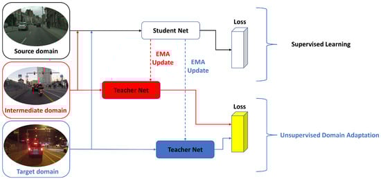
Figure 3.
The Student Net is employed for supervised learning within the source domain, while the Teacher Net serves the purpose of unsupervised learning in both the intermediate and target domains, thereby generating distinct loss functions for each.
To mitigate image style disparities resulting from varying lighting conditions and diverse datasets, we analyzed gray-level co-occurrence matrix values within both the intermediate and target domain images. This analysis contributes to further narrowing the domain gap. Moreover, the frequency information present in the target domain proves valuable for the domain adaptation task. To harness this information, we introduce the Fourier Exponential Decreasing Sampling algorithm. This sampling strategy facilitates the adjustment of the training process of network, aligning it more effectively with the frequency domain characteristics of both the source and target domains.
We adopt the DAFormer work as a benchmark method, leading to significant enhancements in the performance of domain-adaptive semantic segmentation, particularly in challenging ACDC night and foggy scenes. Finally, we optimize the decoder network for efficiency by leveraging group convolution to minimize network parameters. Next, we randomly shuffle the fusion features for the grouped channels to mitigate overfitting in the source domain.
Our contributions are summarized as follows:
(1) Drawing on the concept of grouped convolution, the decoder network is meticulously crafted. This design adjustment results in a remarkable reduction in parameters, shrinking from 3.7 million to 2.66 million, all the while delivering exceptional performance.
(2) The Fourier Exponential Decreasing algorithm is crafted to sample frequency domain information. The sampling strategy for frequency domain information adapts over time through the continuous monitoring of changes in the source domain loss.
(3) Drawing upon the self-training approach detailed in the DAFormer work, we incorporate the reference image as the intermediate domain, while focusing on learning from challenging region proposals.
(4) The UDA algorithm presented in this work demonstrates efficacy not only in enhancing visibility during dark night scenes but also in yielding improved outcomes amidst foggy environments.
2. Related Work
2.1. Semantic Segmentation Network
Semantic segmentation technology finds extensive application within autonomous driving contexts, where its precision profoundly impacts the safety of automated driving systems. A majority of conventional semantic segmentation techniques rely on grayscale image threshold methodologies, encompassing fixed thresholds, the Otsu method, the Canny edge detection algorithm, and region growth strategies. Regrettably, these approaches fall under unsupervised learning methods, rendering them incapable of comprehending the semantic nuances inherent in images. This inherent limitation results in diminished robustness, rendering them susceptible to disruptions originating from the external environment. In 2015, Long et al. introduced the FCN network [17], marking the first use of deep learning for semantic segmentation tasks. This groundbreaking approach outperformed the most advanced semantic segmentation methods of its time. Addressing a limitation of the FCN, Lin et al. introduced the FPN network [18], which leverages a feature pyramid to integrate high-level and shallow semantic information. This innovation significantly enhances semantic segmentation accuracy. Such techniques have also demonstrated effectiveness in studies centered around multi-scale fusion [25,26,27]. In [28], the authors implemented novel strategies including hollow convolution and joint pyramid upsampling, amplifying the receptive field of the network without increasing the convolution size of the kernel. Subsequently, in 2019, DeeplabV3+ [28] combined deep separable convolution, Xception, Encoder-Decoder, FPN, and other technologies, resulting in an impressive 82.1 mIoU performance on the Cityscapes dataset.
Since the introduction of DeeplabV3+, the advancement of semantic segmentation networks has encountered a temporary slowdown. This can be attributed to the limitations of the convolutional kernel, which possesses a relatively small receptive field, thereby impeding the comprehensive assimilation of global image information. To mitigate this challenge, the integration of self-attention mechanisms has surfaced as a promising solution for enabling more efficient acquisition of global contextual information. To better integrate both global and local semantic information, SETR [29] employs the Transformer architecture for the task of semantic segmentation. Inspired by the design principles of the ViT [30] structure, SETR achieved the top rank in the ADE20K dataset competition. When integrating the Transformer structure with a standard convolutional neural network [31], it outperforms conventional convolutional neural networks in semantic segmentation accuracy. However, it is important to note that semantic segmentation networks based on the Transformer structure often face challenges related to excessive computational requirements. In response, researchers have explored methods to make Transformers more light-weight [32,33], aiming to reduce the parameter count of the Transformer architecture while minimizing the impact on accuracy. For instance, the SegFormer network [34], introduced in 2021, achieved an mIoU of 84.00 in the Cityscapes dataset by eliminating location coding and avoiding the use of hollow and ordinary convolutions. Notably, most efforts towards light-weight operation in semantic segmentation network structures, except for SegFormer, have focused on simplifying the potent encoder components, with limited exploration into decoder structure simplification. Consequently, the design of a light-weight decoder network structure holds significant promise, particularly in its application to autonomous driving scenarios in semantic segmentation.
2.2. Adaptation Domain of Adverse Conditions
Numerous domain adaptation methods for semantic segmentation exist [35,36,37], utilizing adversarial learning [38,39,40,41], as commonly understood. Utilizing self-training to generate pseudo-labels tends to outperform adversarial learning [42]. In 2018, Hoffman et al. introduced an inter-domain adaptation model [43] that leverages generative image spatial alignment and latent representation spatial alignment. This model facilitates domain-to-domain guidance through targeted discrimination training task transfers, while also promoting agreement through maintaining semantic consistency before and after adaptation. In 2019, Zou et al. introduced a method called self-training with confidence regularization [44]. This approach employs pseudo-labels as continuous latent variables and enhances domain adaptation performance through iterative joint optimization. The majority of the methods mentioned above are applied within regular domain-to-domain scenarios. However, limited research has been conducted on domain adaptation in adverse domain contexts, particularly concerning adverse scenarios in autonomous driving. Algorithms for removing images captured under adverse conditions in the context of autonomous driving tend to focus predominantly on single-task solutions [45,46,47,48,49]. Within the context of snow scene removal, one can encounter both traditional snow denoising models founded on matrix factorization [50], as well as contemporary deep learning-based approaches, like the deep dense multi-scale network, DDMSNet [51]. This model leverages semantic depth maps to acquire both semantic and geometric awareness, enabling effective snow removal, and the multi-level network, DesnowNet, exhibits the capability to address both translucent and opaque snow particles. Kang et al. introduced a deep learning-based architecture for single-image dehazing. This approach leverages multi-scale residual learning and image decomposition techniques as described by Yeh et al. [52]. The algorithm combines multi-scale deep residual learning with a simplified U-Net architecture to effectively remove haze. Ren et al. employs an end-to-end neural network architecture [53], comprising an encoder and a decoder. This network seamlessly integrates information fusion techniques including white balance, contrast enhancement, and gamma correction. Zhang et al.’s Densely Connected Pyramid Dehazing Network (DCPDN) [54] is intricately woven into the framework, facilitating learning via the atmospheric scattering model.
To recap, there is limited application of domain adaptation techniques in addressing semantic segmentation tasks within challenging scenarios of autonomous driving. Most approaches proactively mitigate the impact of adverse weather conditions and remain focused on single-task objectives. To address these issues, we propose domain adaptation algorithms that are suitable for a variety of adverse weather conditions and achieve excellent performance in night and foggy scenes.
3. Method
3.1. Overview
The task of deep learning domain adaptation involves the necessity for a robust encoder, capable of capturing source domain information effectively in order to enhance the generalization prowess towards target domain information. In our approach, we leverage the potent MiT-B5 [20] network architecture as the foundation, coupled with a reimagined efficient decoder network called ShuffleFormer. With the introduction of a reference image, we extract the challenging pixel mask regions for learning. This augmentation enriches the available information for the domain adaptation task. To optimize the process, the FEDS algorithm dynamically adjusts the sampling strategy based on the source domain loss value. This facilitates the comprehensive learning of frequency characteristics across both source and target domains, ultimately leading to more precise semantic segmentation outcomes. The comprehensive system architecture is visually represented in Figure 4.
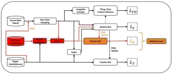
Figure 4.
The black block diagram and lines represent the original method structure of DAFormer, whereas the red block diagram and lines depict our novel approach. Here, the reference images serve as an intermediary domain, contributing to the generation of the loss function.
3.2. ShuffleFormer Network Architecture
In the context of semantic segmentation, the decoder plays a pivotal role in gradually restoring the semantic information image. Enhancing the recognition accuracy of semantic segmentation often involves using techniques such as multi-scale fusion and dilated convolution. The decoder architecture of DAFormer is illustrated in Figure 5a. The inputs , , and within the Hierarchical Transformer structure represent feature maps at distinct scales. These multi-scale feature maps encompass both coarse semantic features and intricate texture details. To facilitate uniformity, all feature maps are standardized in size and channels. Subsequently, a multi-scale dilated convolution, akin to Atrous Spatial Pyramid Pooling (ASPP), is employed for comprehensive multi-scale feature fusion. To achieve multi-scale feature fusion, a multi-scale dilated convolution is employed, drawing parallels to ASPP. Despite incorporating an array of techniques to form a potent decoder in DAFormer, the implementation process becomes overly intricate. Consequently, this paper focuses on optimizing the decoder network with a light-weight approach, ensuring accuracy remains uncompromised. Illustrated in Figure 5b is the ShuffleFormer decoder network, introduced in this study. Initially, and undergo grouped convolutions employing a kernel. This strategic choice significantly reduces the number of network parameters. Subsequently, a post-grouped convolution upsample operation generates feature maps of uniform scale. The culmination of these processes involves the direct fusion of these feature maps. This approach yields a simplified overall network structure while effectively integrating multi-scale semantic information.
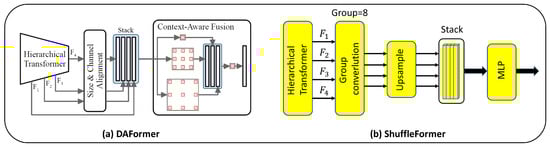
Figure 5.
(a) DAFormer decoder network structure (image quoted from [20]). (b) ShuffleFormer decoder network structure, which is a light-weight operation of semantic segmentation decoder.
The structure of the ShuffleFormer is depicted in Figure 5b. Considering that the network has input channels, output channels, g groups for group convolution, as the size of the convolution kernel, and the network bias uniformly set to False, the parameters for normal convolution, , and grouped convolution, , can be computed as follows:
As shown in Figure 6, when the input and output feature maps share the same size, the total parameter count of a grouped convolutional network is lower compared to standard convolution [55]. In the left side of Figure 6, we have the standard convolution. We assume the input feature map size is , with K convolution kernels generating K output feature maps, each with a convolution kernel size of . Consequently, the parameter count for convolution kernels is . In contrast, the right side of Figure 6 illustrates a grouped convolution. Here, the input size remains , with K output feature maps distributed across g groups. Each group’s input feature map size is , and their output feature maps number . The convolution kernel size becomes . This leads to the grouped convolution network’s total parameter count being only of the standard convolution.
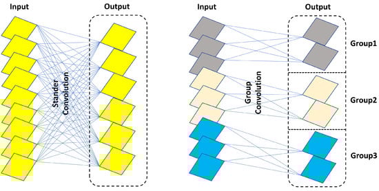
Figure 6.
Comparing standard convolution and group convolution, it is notable that group convolution entails fewer network parameters when the input and output remain consistent.
As shown in Figure 7, we provide an input image with dimensions , which undergoes processing with MiT-B5 to generate multi-scale feature maps. These multi-scale feature maps encompass high-resolution coarse features and low-resolution fine-grained features. This feature combination proves beneficial for semantic segmentation. serves as the input for the decoder network, its dimensions are . The generated feature map , which serves as the input for the decoder network, is of size after undergoing grouped convolution. This step is followed by shuffling to enhance the interaction of semantic information. Once the fusion is complete, the feature map gradually reverts to the size of . Additionally, the multi-scale feature map undergoes upsampling to achieve a uniform size. Subsequently, a concatenation fusion is performed, resulting in an output size of . The final output is obtained through the MLP layer. In our experimentation, we set . For index i belonging to (1,2,3,4), . Additionally, represents the number of classes, which is set to 19. The grouped convolution employs a total of .
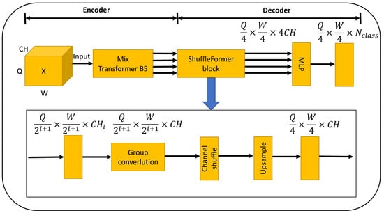
Figure 7.
The comprehensive structure diagram of our semantic segmentation network showcases the use of MiT-B5 architecture for the encoder network, complemented by the ShuffleFormer network structure for the decoder network.
3.3. The Fourier Exponential Decreasing Sampling Algorithm
In the context of semantic segmentation for autonomous driving in adverse weather conditions, it is possible to leverage the Fourier transform algorithm to analyze images in the frequency domain. This analysis can yield valuable semantic information [56]. Low-frequency signals typically correspond to areas in the image where grayscale gradients change gradually. For instance, in scenarios like nighttime and foggy conditions, extensive areas characterized by uniform color blocks fall into the low-frequency region due to their slowly changing grayscale gradients. On the other hand, object boundaries, textures, and image noise contribute to rapid grayscale gradient changes, categorizing them within the high-frequency region. The insights obtained from this frequency domain information can be effectively applied to domain adaptation tasks using the Fourier transform. Regarding Formula (3), it represents the forward discrete Fourier transform formula for the given image, where , the size of the image is , represents the Cartesian coordinates of individual pixel points within the image, and represents the coordinate points of the two-dimensional spectrum obtained through the Fourier transform of the image. Meanwhile, Formula (4) corresponds to the inverse discrete Fourier transform formula applied to the image. The efficient computation of the Fourier transform is detailed in [57].
From top to bottom, Figure 8 displays images depicting daytime, nighttime, and foggy conditions. Additionally, Figure 8a,b illustrate the color image with three channels and the grayscale image with a single channel, respectively. Figure 8c depicts the low-frequency filtered image of the automated driving scene under varying lighting conditions: day, night, and fog. It can be observed that the low-frequency filtered image primarily preserves the textural information related to object edges and image noise points, which are inherent to the high-frequency components of the image. Nevertheless, in areas of the image characterized by low-frequency components, such as extensive regions of solid color patches present in daytime, nighttime, and foggy scenes, these elements have been entirely eradicated. Conversely, Figure 8d illustrates the high-frequency filtered image of the automated driving scene across different lighting conditions: day, night, and fog. It becomes apparent that the high-frequency filtered image retains a majority of the coarse features pertaining to semantic information. For instance, the image still captures the distinctive large color block buildings present within the scene; however, the intricate textural details and noise originally present in the image are now absent.
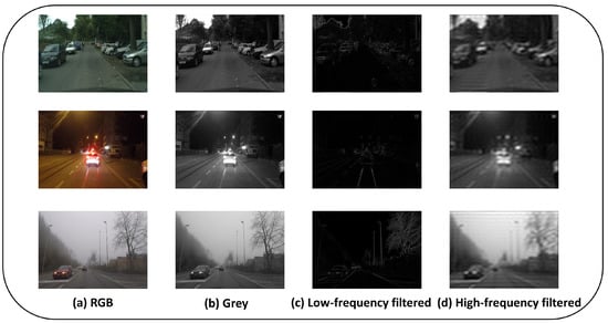
Figure 8.
Fourier-transformed representations of scenes under different atmospheric conditions: clear sky, nighttime, and foggy weather.
By transferring the frequency domain information from the target domain (adverse weather condition) to the images of the source domain (normal weather condition), the source domain images acquire the frequency domain characteristics of the target domain. In addition, training the fused images containing the frequency domain information from the target domain, the neural network incorporates target domain characteristics, thus enhancing the recognition accuracy of autonomous driving systems in adverse weather conditions. In the context of semantic segmentation for autonomous driving, objects like buildings, cars, or pedestrians are identifiable independently of sensors, light sources, or frequency variations. However, in practical scenarios, this interference can disrupt semantic segmentation results, leading to a domain gap between the source and target domains. Interference of this nature is prevalent in images captured during inclement weather conditions. Consequently, approaching the domain adaptation challenge from a frequency domain perspective can enhance the precision of semantic segmentation and recognition for autonomous driving in unfavorable weather conditions.
We refer to the FDA [56] work, given the source dataset (normal weather condition) , where depicts an RGB image and stands for the label of . As above, we assumed for the target data (adverse weather condition), which is not annotated.
After a Fourier transform, we denote the obtained magnitude and phase as and , respectively. represents the image space generated by the inverse Fourier transform of and . In this scenario, the Fourier-transformed image is subjected to a mask denoted as , which zeros out all regions except for the central region. The formulation can be expressed as follows:
We give (normal weather condition) and (adverse weather condition). The Fourier domain adaptation from normal to adverse scenarios can be expressed as follows:
As depicted in Figure 9, the blue region represents the sampling of low-frequency information, while the yellow region corresponds to the sample of high-frequency information. The selection of the high-frequency area is conducted randomly. The FEDS algorithm is capable of adaptively selecting the frequency components to sample from both the source and target domains, based on the current conditions of the network.
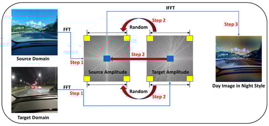
Figure 9.
Upon applying the FEDS algorithm, the source domain image acquires the frequency domain characteristics of the target domain image.
As shown in Equation (7), we refer to the DAFormer [20] loss function calculation method. , , and represent the loss function of the source domain, the loss function of the target domain, and the loss function of the thing-class ImageNet feature distance, respectively. In the FEDS training process, at every 50 iterations of the network, we calculate the difference, denoted as , between the current loss function value of source domain, , and the loss function value, , from the previous 50 iterations. After every 50 iterations of training, we increment the value of K by one, and we let represent the number of iterations of the sampling frequency.
Referencing Algorithm 1, Figure 10 and Figure 11, the value of is computed during iterative training of the network for 50 batches. A positive value signifies underfitting in the source domain learning, necessitating further acquisition of source domain information. In such cases, it is recommended to prioritize learning frequency domain information from the source domain and increase the value of . Conversely, if is non-negative, it indicates the network is appropriately learning source domain information, allowing the sampling algorithm to continue extracting both low- and high-frequency information from the target domain.
| Algorithm 1: The FEDS Algorithm |
| Requirement: source domain and target domain datasets and , as well as a segmentation network . |
| 1. Initialize network parameters randomly. |
| 2. Sampling low-frequency target domain (Operation 2 of Figure 10) |
| 3. For to iter, do |
| 4. Each iteration is conducted 50 times, |
| // Sampling low-frequency target domain (Operation 2 of Figure 10) |
| 5. if , then |
| 6. , run iterations, return step 4 |
| // Sampling low-frequency source domain (Operation 1 of Figure 10) |
| 7. if , then |
| 8. return step 4 |
| // Sampling low-frequency target domain (Operation 2 of Figure 10) |
| 9. if , then |
| 10. , return step 4 |
| // Sampling high-frequency target domain (Operation 3 of Figure 10) |
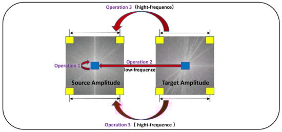
Figure 10.
Schematic diagram of frequency domain sampling of FEDS algorithm: Operation 1 uses low-frequency information in the source domain, operation 2 uses low-frequency information in the target domain, and operation 3 uses high-frequency information in the target domain.
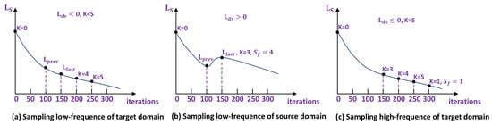
Figure 11.
Three possible cases of the FEDS algorithm: (a) the network training process is normal, (b) the source domain training process is underfitting, (c) the network training process is normal, and high-frequency signals in the target domain are sampled.
3.4. Extraction of Region Proposals from the Reference Image
The reference images within the ACDC dataset hold a wealth of additional information that can be effectively utilized for enhancing semantic segmentation tasks. Figure 12 showcases reference images captured in the ACDC target domain under optimal daytime weather conditions. These images notably augment the available data with supplementary details, serving as intermediary domains to facilitate semantic segmentation in adverse weather. Notably, a domain gap exists between the ideal weather daytime conditions and the challenging bad weather scenarios of the autonomous driving dataset. This divergence can lead to decreased recognition accuracy when applying models trained solely on the former to cross-domain scenes. Addressing this, a strategic approach involves scrutinizing the dissimilarities between the two image sets and guiding the network model to assimilate these divergent cues. This process, in turn, enhances the recognition accuracy of the network model when confronted with challenging weather conditions.
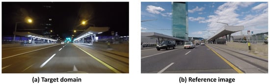
Figure 12.
(a) ACDC night image, (b) ACDC reference image; reference image taken at different times but in the same location, which can serve as an intermediate domain.
The information contained in the gray-level co-occurrence matrix of an image signifies a variety of pixel relationships. By contrasting the gray-level co-occurrence matrices of images captured under optimal and adverse weather conditions, significant dissimilarities in image regions come to light. These distinct regions are selected to guide focused training, ultimately facilitating the acquisition of a network model that mitigates domain gaps. Figure 13 depicts the statistical feature map derived from the gray-level co-occurrence matrices of images captured under ideal and adverse weather conditions. It is apparent that there exist discernible disparities in the standard deviation and entropy values between the two types of images. This discrepancy implies that autonomous driving datasets collected under favorable and inclement weather conditions exhibit notable differences in standard deviation and entropy values during daylight hours. As a strategic measure, we allocate elevated weights to regions characterized by the highest standard deviation and entropy values. These regions are earmarked for the training process, enabling the network to concentrate its learning efforts on challenging areas. Refer to Figure 14 for a detailed exposition of the algorithmic workflow. As follows, the loss function integrates the intermediate domain loss into the original DAFormer work.
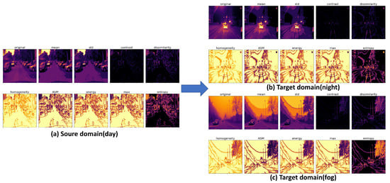
Figure 13.
Comparing the gray-level co-occurrence matrix images between daytime and nighttime, as well as foggy, conditions reveals notable discrepancies in standard deviation and entropy values.
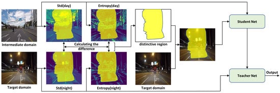
Figure 14.
The reference image serves as the intermediary domain, primarily focusing on extracting the most dissimilar region between this intermediary domain and the target domain. Subsequently, this extracted region is assigned a higher weight during the training process.
As shown in Equation (8), , , and represent the loss function of the source domain, the loss function of the intermediate domain, and the loss function of the target domain, respectively. refers to the physical loss function, as described in the DAFormer method [20], and its coefficient of 0.005 can be adjusted according to the actual situation.
The entropy value of the gray-level co-occurrence matrix signifies the complexity of image information. When the entropy is relatively high, it indicates that the image texture is complex and exhibits significant randomness. Conversely, when the entropy value is low, it indicates that the image texture is simple, with less structural intricacy. Standard deviation reflects the clarity of the image and the depth of the groove lines of the texture. The sharper the texture, the greater the standard deviation. Let represent the gray-level co-occurrence matrix of the image, where i and j are the two-dimensional coordinates of the gray-level formula matrix. We define as the entropy value, as the mean, and as the standard deviation. The formulas for calculating these metrics are provided below:
We designate the matrix X to represent the original image and traverse each pixel in the X matrix, determining the maximum () and minimum () values. The resulting represents the image matrix after undergoing image normalization. represents the upper bound of the desired planning range, while represents the lower bound. corresponds to the maximum pixel value in the image, and represents the minimum pixel value. By applying the following formula (12), setting to 255 and to 0, we can effectively normalize the image data to fit within the range of 0 to 255.
We employ a method based on comparing standard deviations and entropy maps to analyze scenes in both normal and non-ideal conditions at identical locations. This comparison allows us to identify the most salient regions, which are then assigned higher contribution weights during the training process. This concept is illustrated in Figure 14.
The process of mask generation involves two main steps. The initial step entails computing the difference in standard deviations within the image. In this step, a threshold for standard deviations is established. When the standard deviation of an image pixel surpasses this threshold, the corresponding area is designated as a . The second step focuses on determining the disparity in entropy values. Entropy values are computed for both the scenario with non-ideal conditions in the target domain and the normal scenario in the intermediate domain. Subsequently, a comparison is made between these two entropy values, utilizing a predefined threshold. This aids in identifying the region with the highest information content, which serves as the . Assuming the input image for the reference image is denoted as and the output image as , the intersection of these two masks is utilized to compute the weight applied to . The formula for this computation is as follows:
The specific algorithm process is outlined in Algorithm 2. Firstly, the standard deviation and entropy values of the middle domain and the target domain are calculated to obtain , , , and . Afterward, the differences between the two are computed to derive and , identifying regions with substantial disparities between the middle and target domains. It is noteworthy that and may contain outlier noise points, potentially impacting the screening of candidate regions. To address this, the algorithm employs a median filtering technique for smoothing.
Before proceeding with candidate region screening, the image is normalized to the 0–255 value range, resulting in and . A thresholding step follows, where pixel values exceeding 127.5 are set to 1; otherwise, they are set to 0, yielding binary masks and . Finally, utilizing Equation (13), the images are fused, producing as the ultimate fused image.
Subsequently, the most significant region within the intermediate domain can be acquired. Lastly, to ensure that pixel values remain within an acceptable range, a renormalization operation is performed.
| Algorithm 2: Extraction of Region Proposals |
| Requirement: intermediate domain and target domain datasets and . |
| 1. Calculate the standard deviation and entropy |
| 2. Calculating the difference |
| 3. Median filtering |
| 4. Image normalization |
| 5. Generate the mask image, threshold |
| 6. Image fusion |
4. Experiments
4.1. Experimental Details
Datasets: For the source domain dataset, we utilized the Cityscapes dataset, comprising 2975 training samples and 500 validation samples, each with a resolution of 2048 × 1024 pixels. For the target domain dataset, we employed the ACDC dataset, consisting of 400 training samples and 500 validation samples, capturing both night, foggy, rainy, and snowy scenes, with a resolution of 1920 × 1080 pixels. During training and validation, we consistently resized the images to dimensions of 512 × 512 pixels.
Network Architecture: To mitigate the bias introduced by relying solely on experimental results from a single encoder network, we employed both Mix Transformer B5 (MiT-B5) [20] and ResNet-101 [58] as encoding networks. These choices are based on the mmsegmentation framework, and we utilized the ImageNet-1K dataset for pre-training. The output channels of MiT-B5 are configured as C = [64, 128, 320, 512].
Training: To ensure consistency and avoid interference from varying hyperparameter values, we aligned our training approach with that of the DAFormer work. Specifically, we set the encoder learning rate to and the decoder learning rate to . Weight decay is employed with a coefficient of 0.01. Following the warm-up phase, we implemented linear decay to mitigate potential overfitting caused by the limited dataset size. The total training iteration count is 20,000. It is worth noting that the original DAFormer work utilized 40,000 iterations for training. The computational hardware employed for calculations is the Tesla M40 24G graphics card.
4.2. ShuffleFormer Performance Test
To evaluate the domain adaptation performance of the ShuffleFormer network as the decoder of a segmentation network under challenging conditions and to mitigate the bias introduced by a single encoder, we utilized ResNet-101 [58] and MiT-B5 [20] architectures, following the approach outlined in the DAFormer work. All the methodologies employed in this experiment were validated using the ACDC night scene dataset. As demonstrated in the first and seventh rows of Table 1, it is evident that the performance of the SegFormer768 decoder, which employs a fully connected network structure, lags behind that of the decoder utilizing similar ASPP multi-scale extraction features. In scenes of severe weather conditions, semantic segmentation images suffer from substantial interference from extraneous information, thereby escalating the neural network’s learning complexity. Consequently, the network’s recognition accuracy diminishes. The SegFormer768 [34], functioning as a straightforward decoder, inadequately captures the intricacies of semantic segmentation. Conversely, architectures like UperNet256, UperNet512 [59], DAFormer aspp, and DAFormer seaspp [20] demonstrate improved performance. These decoders leverage ASPP-like structures to effectively extract high-resolution coarse features crucial for semantic segmentation, along with low-resolution fine texture features. Remarkably, the DAFormer seaspp decoder outperforms the DAFormer aspp decoder while utilizing fewer parameters (as demonstrated in the fourth and fifth rows of Table 1, as well as the tenth and eleventh rows of Table 1). This phenomenon can be attributed to the implementation of depthwise separable convolutions in the DAFormer sesapp decoder. This approach fosters a lighter convolutional neural network architecture, mitigating overfitting in the source domain. Similarly, although the ShuffleFormer lacks an ASPP-like structure, it excels in this experiment by adopting a grouped convolution structure with fewer parameters than the depthwise separable convolution. This outcome substantiates the validity of this hypothesis.

Table 1.
Comparison of ShuffleFormer and mainstream decoder network performance (ACDC night).
The ShuffleFormer network not only reduces the number of network parameters but also addresses intricate design considerations for the decoder network structure. Elaborate decoders can inadvertently lead to overfitting on source domain data, consequently impeding the efficacy of unsupervised domain adaptation and undermining the accuracy of the network in the target domain.
4.3. Cityscapes –> ACDC Night
Table 2 presents a comparison of domain adaptation capabilities, specifically addressing the transition from the source domain of the Cityscapes night scene to the target domain of ACDC adverse scene. Utilizing ResNet-101 as the encoder yields notably inferior performance compared to the Transformer-based MiT-B5 model. This observation reinforces the validity of the earlier-stated hypothesis, Transformers pay more attention to the global information of the image than CNNS, highlighting that the Transformer architecture proves more advantageous for domain adaptation in dark night scenes.
Table 2.
Comparison of ACDC night experimental results. Ref: The reference image is used as an intermediate domain for training. Region Proposal: This involves focusing the training process on candidate regions within the intermediate domain image. FEDS: This abbreviation stands for the Fourier Index Decreasing Algorithm, which is used to enhance our method.
Building upon the MiT-B5 model, the introduction of reference images (as demonstrated in the first and second rows of Table 2, as well as the fifth and sixth rows of Table 2) results in a noteworthy increase of 1.01% and 2.34% in mIoU, respectively. This introduction capitalizes on the wealth of semantic information contained within the intermediate domain of the target domain, and the intermediate domain contains information that is not available in adverse weather conditions, thus effectively enhancing the domain adaptation capability in adverse weather conditions of the network.
Upon examining the third and seventh rows of Table 2, it becomes evident that the standard deviation and entropy of the gray-level co-occurrence matrix aptly reflect the distinctions between the intermediate domain and the target domain. The variations in standard deviation and entropy substantiate the notion that incorporating information via the training process improves performance. Specifically, ResNet-101 demonstrates a 2.61% improvement as an encoder, and MiT-B5 displays a 2.12% increase as an encoder, further attesting to the superior recognition accuracy of MiT-B5 when embedded within a Transformer encoder structure in low-light scenarios.
The efficacy of the FEDS algorithm becomes evident through the examination of the third and fourth rows of Table 2, as well as the seventh and eighth rows of Table 2. The adoption of the FEDS algorithm leads to enhanced recognition accuracy, with ResNet-101 as an encoder experiencing a 1.20% improvement and MiT-B5 as an encoder realizing a 2.31% advancement. The integration of low-frequency signals from the target domain is particularly advantageous in mitigating the domain gap in cross-domain tasks. In the context of autonomous driving in dark scenes, the low-frequency signals capture distinct features, such as large color patches that contrast starkly with daytime scenes. However, the presence of low-light conditions, coupled with optical factors like camera sensors, can blur semantic information related to objects like bicycles, buses, and roads. Additionally, night scenes are prone to introducing discrete noise points. By incorporating high-frequency signals from the target domain, sampled via Fourier transform and fused with the source domain during training, the neural network becomes more resilient and attains improved performance in low-light environments. We employ the DAFormer work as a benchmark for comparison. As a result, the mean Intersection over Union (mIoU) on the ACDC dark night scene test dataset increases from 44.34% to 51.11%.
Figure 15 illustrates the semantic segmentation outcomes of the ACDC night. It shows that our method improves both domain adaptation tasks in dark night scenes.
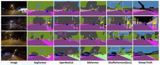
Figure 15.
Qualitative results on ACDC night. The yellow rectangular boxes represent the regions where our method has better segmentation performance than the mainstream semantic segmentation methods. Our method improves the segmentation accuracy for both small objects and background.
4.4. Cityscapes –> ACDC Fog
Table 3 presents the experimental data conducted in a foggy autonomous driving scenario. Notably, our method, as outlined in this paper, exhibits a discernible enhancement in recognition accuracy for semantic segmentation within the foggy environment. A comparative analysis of the first and second rows as well as the fifth and sixth rows of Table 3 highlights that the incorporation of the intermediate domain contributes to an increment of 3.55% and 3.20% in mIoU, respectively. It is noteworthy that upon introducing the intermediate domain, the network model demonstrates enhanced adaptability in handling foggy scenes. The presence of fine fog particles and noise in the foggy scene, particularly around the camera, poses a challenge to the accuracy of semantic segmentation. Introducing an intermediate domain as a reference in clear daytime scenes can be beneficial for improving recognition accuracy. Further scrutiny of Table 3 reveals a similar pattern between the second and third rows, along with the sixth and seventh rows. Specifically, dedicating attention to the region of interest within the intermediate of the foggy scene domain translates to an accuracy improvement, resulting in a 1.25% mIoU increase and a 1.37% mIoU increase, respectively. There are large areas of color blocks in the foggy scene, and the fog distribution is more uniform compared to the night scene. Therefore, there is little difference between the entropy and contrast of the gray-level co-occurrence matrix in the foggy scene, and the candidate regions to be trained extracted by entropy and contrast are not obvious. Lastly, the incorporation of the FEDS algorithm into the training process yields a discernible, albeit not prominently pronounced, enhancement in semantic segmentation accuracy. This observation indicates that while domain adaptation employing spectrum analysis proves effective in the foggy scene context, the degree of improvement might not be highly conspicuous. We employ the DAFormer framework as a benchmark for comparison. As a result, the mean Intersection over Union (mIoU) on the foggy scene test dataset rises from 50.51% to 55.85%.
Table 3.
Comparison of ACDC fog experimental results. Ref: The reference image is used as an intermediate domain for training. Region Proposal: This involves focusing the training process on candidate regions within the intermediate domain image. FEDS: This abbreviation stands for the Fourier Index Decreasing Algorithm, which is used to enhance our method.
Figure 16 illustrates the semantic segmentation outcomes of the ACDC fog. It shows that our method improves both domain adaptation tasks in fog scenes.
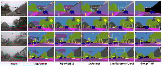
Figure 16.
Qualitative results on ACDC fog. The yellow rectangular boxes represent the regions where our method has better segmentation performance compared to the mainstream semantic segmentation methods. Our method has a certain improvement in segmentation accuracy for color patches with large areas.
4.5. Cityscapes –> ACDC Rain and Snow
Table 4 and Table 5 present the experimental results of ACDC under rainy and snowy conditions. The findings demonstrate that our method consistently achieves commendable semantic segmentation results in such challenging scenarios. Specifically, we observed an increase of 6.36% in mIoU for rainy scenes and 5.93% for snowy scenes.
Table 4.
Comparison of ACDC rain experimental results.
Table 5.
Comparison of ACDC snow experimental results.
Figure 17 and Figure 18 illustrate the notable improvement in the semantic segmentation performance of our method in rainy and snowy scenes when compared to the leading network. When compared to the DAFormer method, our approach demonstrates a significant enhancement in semantic segmentation performance under adverse weather conditions, due to the incorporation of intermediate domain information. To ensure robustness and mitigate reliance on the Transformer network, we employ ResNet-101 as the backbone for comparison. The experimental results affirm a substantial improvement in the performance of our method for semantic segmentation in rainy and snowy scenes.
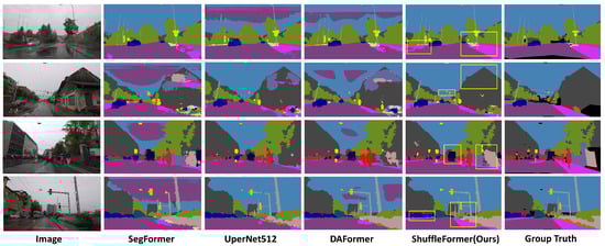
Figure 17.
Qualitative results on ACDC rain. The yellow rectangular boxes represent the regions where our method has better segmentation performance compared to the mainstream semantic segmentation methods.
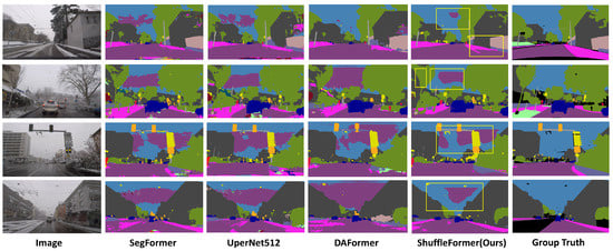
Figure 18.
Qualitative results on ACDC snow. The yellow rectangular boxes represent the regions where our method has better segmentation performance compared to the mainstream semantic segmentation methods.
5. Conclusions
Our method proves effective in semantic segmentation scenarios involving night, foggy, rainy, and snowy scenes. Additionally, the use of candidate region training and the FEDS algorithm yields favorable results in night scenes, although its effectiveness in foggy scenes is less prominent. The proposed ShuffleFormer architecture in this paper, which integrates a Transformer-based encoder and a decoder featuring contextual feature fusion, demonstrates efficacy in addressing semantic segmentation challenges within adverse scenarios relevant to autonomous driving. Additionally, we have introduced auxiliary training involving reference images from favorable weather conditions, specifically night and foggy scenes in autonomous driving scenarios. This augmentation enables the network to assimilate supplementary information, consequently enhancing its capacity to achieve superior segmentation outcomes. Moreover, with regard to the frequency domain, we extract low-frequency information from the target domain scene and integrate it into the source domain images, a strategy that substantially contributes to segmentation quality.
Through an array of experiments, our approach has been substantiated as well-suited for adaptive tasks within the realm of autonomous driving. It boasts commendable performance, with the designed ShuffleFormer network embodying a balance between simplicity and efficiency. While the ShuffleFormer network, as devised in this study, boasts a compact parameter count, its efficacy in terms of computational efficiency on mainstream chips is somewhat lacking. Empirical testing indicates that the chip consumes a considerable amount of memory, and the majority of chips are currently optimized for standard convolutional neural networks. We expect that mainstream chips will progressively offer enhanced support for light-weight neural networks in the imminent future.
Furthermore, although the algorithm introduced in this paper holds potential applicability across various adverse weather autonomous driving scenarios, it is important to note that the experiments herein solely focus on night, foggy, rainy, and snowy scenes of the ACDC dataset. Given the constraints of time and data volume, the effectiveness of the algorithm in other adverse weather autonomous driving datasets remains an area that warrants further investigation.
Author Contributions
X.C.: conceptualization, methodology, investigation, visualization, writing—original draft preparation; N.J.: software, data curation, validation, investigation; Y.L.: characterization, resources, investigation; G.C.: formal analysis, resources; Z.L.: visualization, data curation; Z.Y.: supervision, funding acquisition; Q.Z.: supervision, writing—review and editing, software; R.Z.: project administration, methodology, supervision. All authors have read and agreed to the published version of the manuscript.
Funding
This research is supported by FDCT under its General R&D Subsidy Program Fund (Grant No. 0038/2022/A), Macau.
Data Availability Statement
Publicly available datasets were analyzed in this study. These data can be found in https://acdc.vision.ee.ethz.ch/ and https://www.cityscapes-dataset.com/(accessed on 15 June 2023).
Conflicts of Interest
Author Zheng Liang was employed by the company Celedyne Technologies Co., Ltd. Author Runsheng Zhao was employed by the company National Instruments Corporation. The remaining authors declare that the re-search was conducted in the absence of any commercial or financial relationships that could be construed as a potential conflict of interest.
References
- Karmouni, H.; Jahid, T.; El Affar, I.; Sayyouri, M.; Hmimid, A.; Qjidaa, H.; Rezzouk, A. Image analysis using separable Krawtchouk-Tchebichef’s moments. In Proceedings of the 2017 International Conference on Advanced Technologies for Signal and Image Processing (ATSIP), Fez, Morocco, 22–24 May 2017; pp. 1–5. [Google Scholar]
- Avazov, K.; Mukhiddinov, M.; Makhmudov, F.; Cho, Y.I. Fire detection method in smart city environments using a deep-learning-based approach. Electronics 2021, 11, 73. [Google Scholar] [CrossRef]
- Hmimid, A.; Sayyouri, M.; Qjidaa, H. Image classification using separable invariant moments of Charlier-Meixner and support vector machine. Multimed. Tools Appl. 2018, 77, 23607–23631. [Google Scholar] [CrossRef]
- Pal, R.; Mukhopadhyay, S.; Chakraborty, D.; Suganthan, P.N. A Hybrid Algorithm for Urban LULC Change Detection for Building Smart-city by Using WorldView Images. IETE J. Res. 2023, 69, 5748–5754. [Google Scholar] [CrossRef]
- Jahid, T.; Karmouni, H.; Hmimid, A.; Sayyouri, M.; Qjidaa, H. Image moments and reconstruction by Krawtchouk via Clenshaw’s reccurence formula. In Proceedings of the 2017 International Conference on Electrical and Information Technologies (ICEIT), Rabat, Moroccan, 15–18 November 2017; pp. 1–7. [Google Scholar]
- Malik, S.; Khan, M.A.; El-Sayed, H.; Khan, M.J. Should Autonomous Vehicles Collaborate in a Complex Urban Environment or Not? Smart Cities 2023, 6, 2447–2483. [Google Scholar] [CrossRef]
- Yang, X.; Ahemd, H.U.; Huang, Y.; Lu, P. Cumulatively Anticipative Car-Following Model with Enhanced Safety for Autonomous Vehicles in Mixed Driver Environments. Smart Cities 2023, 6, 2260–2281. [Google Scholar] [CrossRef]
- Ahmed, H.U.; Huang, Y.; Lu, P.; Bridgelall, R. Technology Developments and Impacts of Connected and Autonomous Vehicles: An Overview. Smart Cities 2022, 5, 382–404. [Google Scholar] [CrossRef]
- Sun, P.; Kretzschmar, H.; Dotiwalla, X.; Chouard, A.; Patnaik, V.; Tsui, P.; Guo, J.; Zhou, Y.; Chai, Y.; Caine, B.; et al. Scalability in perception for autonomous driving: Waymo open dataset. In Proceedings of the IEEE/CVF Conference on Computer Vision and Pattern Recognition, Seattle, WA, USA, 13–19 June 2020; pp. 2446–2454. [Google Scholar]
- Caesar, H.; Bankiti, V.; Lang, A.H.; Vora, S.; Liong, V.E.; Xu, Q.; Krishnan, A.; Pan, Y.; Baldan, G.; Beijbom, O. nuscenes: A multimodal dataset for autonomous driving. In Proceedings of the IEEE/CVF Conference on Computer Vision and Pattern Recognition, Seattle, WA, USA, 13–19 June 2020; pp. 11621–11631. [Google Scholar]
- Shao, H.; Wang, L.; Chen, R.; Li, H.; Liu, Y. Safety-enhanced autonomous driving using interpretable sensor fusion transformer. In Proceedings of the Conference on Robot Learning PMLR, Atlanta, GA, USA, 6–9 November 2023; pp. 726–737. [Google Scholar]
- Wang, H.; Chen, Y.; Cai, Y.; Chen, L.; Li, Y.; Sotelo, M.A.; Li, Z. SFNet-N: An improved SFNet algorithm for semantic segmentation of low-light autonomous driving road scenes. IEEE Trans. Intell. Transp. Syst. 2022, 23, 21405–21417. [Google Scholar] [CrossRef]
- Muhammad, K.; Hussain, T.; Ullah, H.; Del Ser, J.; Rezaei, M.; Kumar, N.; Hijji, M.; Bellavista, P.; de Albuquerque, V.H.C. Vision-based semantic segmentation in scene understanding for autonomous driving: Recent achievements, challenges, and outlooks. IEEE Trans. Intell. Transp. Syst. 2022, 23, 22694–22715. [Google Scholar] [CrossRef]
- Chen, C.; Wang, C.; Liu, B.; He, C.; Cong, L.; Wan, S. Edge Intelligence Empowered Vehicle Detection and Image Segmentation for Autonomous Vehicles. IEEE Trans. Intell. Transp. Syst. 2023, 24, 13023–13034. [Google Scholar] [CrossRef]
- Cordts, M.; Omran, M.; Ramos, S.; Rehfeld, T.; Enzweiler, M.; Benenson, R.; Franke, U.; Roth, S.; Schiele, B. The cityscapes dataset for semantic urban scene understanding. In Proceedings of the IEEE Conference on Computer Vision and Pattern Recognition, Las Vegas, NV, USA, 27–30 June 2016; pp. 3213–3223. [Google Scholar]
- Reddy, N.; Singhal, A.; Kumar, A.; Baktashmotlagh, M.; Arora, C. Master of all: Simultaneous generalization of urban-scene segmentation to all adverse weather conditions. In Proceedings of the European Conference on Computer Vision, Tel Aviv, Israel, 23 October 2022; Springer Nature: Cham, Switzerland, 2022; pp. 51–69. [Google Scholar]
- Long, J.; Shelhamer, E.; Darrell, T. Fully convolutional networks for semantic segmentation. In Proceedings of the IEEE Conference on Computer Vision and Pattern Recognition, Boston, MA, USA, 7–12 June 2015; pp. 3431–3440. [Google Scholar]
- Lin, T.Y.; Dollár, P.; Girshick, R.; He, K.; Hariharan, B.; Belongie, S. Feature pyramid networks for object detection. In Proceedings of the IEEE Conference on Computer Vision and Pattern Recognition, Honolulu, HI, USA, 21–26 July 2017; pp. 2117–2125. [Google Scholar]
- Jain, J.; Li, J.; Chiu, M.T.; Hassani, A.; Orlov, N.; Shi, H. Oneformer: One transformer to rule universal image segmentation. In Proceedings of the IEEE/CVF Conference on Computer Vision and Pattern Recognition, Vancouver, BC, Canada, 17–24 June 2023; pp. 2989–2998. [Google Scholar]
- Hoyer, L.; Dai, D.; Van Gool, L. Daformer: Improving network architectures and training strategies for domain-adaptive semantic segmentation. In Proceedings of the IEEE/CVF Conference on Computer Vision and Pattern Recognition, New Orleans, LA, USA, 18–24 June 2022; pp. 9924–9935. [Google Scholar]
- Richter, S.R.; Vineet, V.; Roth, S.; Koltun, V. Playing for data: Ground truth from computer games. In Proceedings of the Computer Vision–ECCV 2016: 14th European Conference, Amsterdam, The Netherlands, 11–14 October 2016; Proceedings, Part II 14. Springer International Publishing: Berlin/Heidelberg, Germany, 2016; pp. 102–118. [Google Scholar]
- Sakaridis, C.; Dai, D.; Van Gool, L. ACDC: The adverse conditions dataset with correspondences for semantic driving scene understanding. In Proceedings of the IEEE/CVF International Conference on Computer Vision, Montreal, BC, Canada, 11–17 October 2021; pp. 10765–10775. [Google Scholar]
- Sakaridis, C.; Dai, D.; Van Gool, L. Map-guided curriculum domain adaptation and uncertainty-aware evaluation for semantic nighttime image segmentation. IEEE Trans. Pattern Anal. Mach. Intell. 2020, 44, 3139–3153. [Google Scholar] [CrossRef]
- Burnett, K.; Yoon, D.J.; Wu, Y.; Li, A.Z.; Zhang, H.; Lu, S.; Qian, J.; Tseng, W.K.; Lambert, A.; Leung, K.Y.; et al. Boreas: A multi-season autonomous driving dataset. Int. J. Robot. Res. 2023, 42, 33–42. [Google Scholar] [CrossRef]
- Lin, G.; Milan, A.; Shen, C.; Reid, I. Refinenet: Multi-path refinement networks for high-resolution semantic segmentation. In Proceedings of the IEEE Conference on Computer Vision and Pattern Recognition, Honolulu, HI, USA, 21–26 July 2017; pp. 1925–1934. [Google Scholar]
- Wang, J.; Sun, K.; Cheng, T.; Jiang, B.; Deng, C.; Zhao, Y.; Liu, D.; Mu, Y.; Tan, M.; Wang, X.; et al. Deep high-resolution representation learning for visual recognition. IEEE Trans. Pattern Anal. Mach. Intell. 2020, 43, 3349–3364. [Google Scholar] [CrossRef] [PubMed]
- Sun, K.; Zhao, Y.; Jiang, B.; Cheng, T.; Xiao, B.; Liu, D.; Mu, Y.; Wang, X.; Liu, W.; Wang, J. High-resolution representations for labeling pixels and regions. arXiv 2019, arXiv:1904.04514. [Google Scholar]
- Yang, M.; Yu, K.; Zhang, C.; Li, Z.; Yang, K. Denseaspp for semantic segmentation in street scenes. In Proceedings of the IEEE Conference on Computer Vision and Pattern Recognition, Salt Lake City, UT, USA, 18–23 June 2018; pp. 3684–3692. [Google Scholar]
- Zheng, S.; Lu, J.; Zhao, H.; Zhu, X.; Luo, Z.; Wang, Y.; Fu, Y.; Feng, J.; Xiang, T.; Torr, P.H.; et al. Rethinking semantic segmentation from a sequence-to-sequence perspective with transformers. In Proceedings of the IEEE/CVF Conference on Computer Vision and Pattern Recognition, Nashville, TN, USA, 20–25 June 2021; pp. 6881–6890. [Google Scholar]
- Dosovitskiy, A.; Beyer, L.; Kolesnikov, A.; Weissenborn, D.; Zhai, X.; Unterthiner, T.; Dehghani, M.; Minderer, M.; Heigold, G.; Gelly, S.; et al. An image is worth 16x16 words: Transformers for image recognition at scale. arXiv 2020, arXiv:2010.11929. [Google Scholar]
- Chen, J.; Lu, Y.; Yu, Q.; Luo, X.; Adeli, E.; Wang, Y.; Lu, L.; Yuille, A.L.; Zhou, Y. Transunet: Transformers make strong encoders for medical image segmentation. arXiv 2021, arXiv:2102.04306. [Google Scholar]
- Mehta, S.; Rastegari, M. Mobilevit: Light-weight, general-purpose, and mobile-friendly vision transformer. arXiv 2021, arXiv:2110.02178. [Google Scholar]
- Zhang, W.; Huang, Z.; Luo, G.; Chen, T.; Wang, X.; Liu, W.; Yu, G.; Shen, C. TopFormer: Token pyramid transformer for mobile semantic segmentation. In Proceedings of the IEEE/CVF Conference on Computer Vision and Pattern Recognition, New Orleans, LA, USA, 18–24 June 2022; pp. 12083–12093. [Google Scholar]
- Xie, E.; Wang, W.; Yu, Z.; Anandkumar, A.; Alvarez, J.M.; Luo, P. SegFormer: Simple and efficient design for semantic segmentation with transformers. Adv. Neural Inf. Process. Syst. 2021, 34, 12077–12090. [Google Scholar]
- Ruan, C.; Wang, W.; Hu, H.; Chen, D. Category-Level Adversaries for Semantic Domain Adaptation. IEEE Access 2019, 7, 83198–83208. [Google Scholar] [CrossRef]
- Sankaranarayanan, S.; Balaji, Y.; Jain, A.; Lim, S.N.; Chellappa, R. Learning From Synthetic Data: Addressing Domain Shift for Semantic Segmentation. In Proceedings of the IEEE Conference on Computer Vision and Pattern Recognition (CVPR), Salt Lake City, UT, USA, 18–23 June 2018. [Google Scholar]
- Wang, Z.; Yu, M.; Wei, Y.; Feris, R.; Xiong, J.; Hwu, W.m.; Huang, T.S.; Shi, H. Differential Treatment for Stuff and Things: A Simple Unsupervised Domain Adaptation Method for Semantic Segmentation. In Proceedings of the IEEE/CVF Conference on Computer Vision and Pattern Recognition (CVPR), Seattle, WA, USA, 13–19 June 2020. [Google Scholar]
- Vu, T.H.; Jain, H.; Bucher, M.; Cord, M.; Perez, P. ADVENT: Adversarial Entropy Minimization for Domain Adaptation in Semantic Segmentation. In Proceedings of the IEEE/CVF Conference on Computer Vision and Pattern Recognition (CVPR), Long Beach, CA, USA, 15–20 June 2019. [Google Scholar]
- Tsai, Y.H.; Hung, W.C.; Schulter, S.; Sohn, K.; Yang, M.H.; Chandraker, M. Learning to adapt structured output space for semantic segmentation. In Proceedings of the IEEE Conference on Computer Vision and Pattern Recognition, Salt Lake City, UT, USA, 18–23 June 2018; pp. 7472–7481. [Google Scholar]
- Creswell, A.; White, T.; Dumoulin, V.; Arulkumaran, K.; Sengupta, B.; Bharath, A.A. Generative adversarial networks: An overview. IEEE Signal Process. Mag. 2018, 35, 53–65. [Google Scholar] [CrossRef]
- Ganin, Y.; Ustinova, E.; Ajakan, H.; Germain, P.; Larochelle, H.; Laviolette, F.; Marchand, M.; Lempitsky, V. Domain-adversarial training of neural networks. J. Mach. Learn. Res. 2016, 17, 1–35. [Google Scholar]
- Zhang, P.; Zhang, B.; Zhang, T.; Chen, D.; Wang, Y.; Wen, F. Prototypical pseudo label denoising and target structure learning for domain adaptive semantic segmentation. In Proceedings of the 2021 IEEE/CVF Conference on Computer Vision and Pattern Recognition (CVPR), Nashville, TN, USA, 20–25 June 2021; pp. 12414–12424. [Google Scholar]
- Hoffman, J.; Tzeng, E.; Park, T.; Zhu, J.Y.; Isola, P.; Saenko, K.; Efros, A.; Darrell, T. Cycada: Cycle-consistent adversarial domain adaptation. In Proceedings of the International Conference on Machine Learning, PMLR, Stockholmsmassan, Stockholm, Sweden, 10–15 July 2018; pp. 1989–1998. [Google Scholar]
- Zou, Y.; Yu, Z.; Liu, X.; Kumar, B.; Wang, J. Confidence regularized self-training. In Proceedings of the IEEE/CVF International Conference on Computer Vision, Long Beach, CA, USA, 15–20 June 2019; pp. 5982–5991. [Google Scholar]
- Li, B.; Peng, X.; Wang, Z.; Xu, J.; Feng, D. Aod-net: All-in-one dehazing network. In Proceedings of the IEEE International Conference on Computer Vision, Venice, Italy, 22–29 October 2017; pp. 4770–4778. [Google Scholar]
- Gao, H.; Guo, J.; Wang, G.; Zhang, Q. Cross-domain correlation distillation for unsupervised domain adaptation in nighttime semantic segmentation. In Proceedings of the IEEE/CVF Conference on Computer Vision and Pattern Recognition, New Orleans, LA, USA, 18–24 June 2022; pp. 9913–9923. [Google Scholar]
- Deng, X.; Wang, P.; Lian, X.; Newsam, S. NightLab: A dual-level architecture with hardness detection for segmentation at night. In Proceedings of the IEEE/CVF Conference on Computer Vision and Pattern Recognition, New Orleans, LA, USA, 18–24 June 2022; pp. 16938–16948. [Google Scholar]
- Iqbal, J.; Hafiz, R.; Ali, M. FogAdapt: Self-supervised domain adaptation for semantic segmentation of foggy images. Neurocomputing 2022, 501, 844–856. [Google Scholar] [CrossRef]
- Lee, S.; Son, T.; Kwak, S. Fifo: Learning fog-invariant features for foggy scene segmentation. In Proceedings of the IEEE/CVF Conference on Computer Vision and Pattern Recognition, New Orleans, LA, USA, 18–24 June 2022; pp. 18911–18921. [Google Scholar]
- Ren, W.; Tian, J.; Han, Z.; Chan, A.; Tang, Y. Video desnowing and deraining based on matrix decomposition. In Proceedings of the IEEE Conference on Computer Vision and Pattern Recognition, Honolulu, HI, USA, 21–26 July 2017; pp. 4210–4219. [Google Scholar]
- Zhang, K.; Li, R.; Yu, Y.; Luo, W.; Li, C. Deep dense multi-scale network for snow removal using semantic and depth priors. IEEE Trans. Image Process. 2021, 30, 7419–7431. [Google Scholar] [CrossRef] [PubMed]
- Yeh, C.H.; Huang, C.H.; Kang, L.W. Multi-scale deep residual learning-based single image haze removal via image decomposition. IEEE Trans. Image Process. 2019, 29, 3153–3167. [Google Scholar] [CrossRef] [PubMed]
- Ren, W.; Ma, L.; Zhang, J.; Pan, J.; Cao, X.; Liu, W.; Yang, M.H. Gated fusion network for single image dehazing. In Proceedings of the IEEE Conference on Computer Vision and Pattern Recognition, Salt Lake City, UT, USA, 18–23 June 2018; pp. 3253–3261. [Google Scholar]
- Zhang, H.; Patel, V.M. Densely connected pyramid dehazing network. In Proceedings of the IEEE Conference on Computer Vision and Pattern Recognition, Salt Lake City, UT, USA, 18–23 June 2018; pp. 3194–3203. [Google Scholar]
- Zhang, X.; Zhou, X.; Lin, M.; Sun, J. Shufflenet: An extremely efficient convolutional neural network for mobile devices. In Proceedings of the IEEE Conference on Computer Vision and Pattern Recognition, Salt Lake City, UT, USA, 18–23 June 2018; pp. 6848–6856. [Google Scholar]
- Yang, Y.; Soatto, S. Fda: Fourier domain adaptation for semantic segmentation. In Proceedings of the IEEE/CVF Conference on Computer Vision and Pattern Recognition, Seattle, WA, USA, 13–19 June 2020; pp. 4085–4095. [Google Scholar]
- Frigo, M.; Johnson, S.G. FFTW: An adaptive software architecture for the FFT. In Proceedings of the 1998 IEEE International Conference on Acoustics, Speech and Signal Processing, ICASSP’98 (Cat. No. 98CH36181), Seattle, WA, USA, 15 May 1998; Volume 3, pp. 1381–1384. [Google Scholar]
- He, K.; Zhang, X.; Ren, S.; Sun, J. Deep residual learning for image recognition. In Proceedings of the IEEE Conference on Computer Vision and Pattern Recognition, Las Vegas, NV, USA, 27–30 June 2016; pp. 770–778. [Google Scholar]
- Xiao, T.; Liu, Y.; Zhou, B.; Jiang, Y.; Sun, J. Unified perceptual parsing for scene understanding. In Proceedings of the European Conference on Computer Vision (ECCV); 2018; pp. 418–434. [Google Scholar]
Disclaimer/Publisher’s Note: The statements, opinions and data contained in all publications are solely those of the individual author(s) and contributor(s) and not of MDPI and/or the editor(s). MDPI and/or the editor(s) disclaim responsibility for any injury to people or property resulting from any ideas, methods, instructions or products referred to in the content. |
© 2024 by the authors. Licensee MDPI, Basel, Switzerland. This article is an open access article distributed under the terms and conditions of the Creative Commons Attribution (CC BY) license (https://creativecommons.org/licenses/by/4.0/).