


Abstract
Waterflooding in oilfields for oil displacement and reservoir pressure maintenance has led to the production of scale in several reservoirs. The formation of scale occurs both in the porous media of the reservoir and in the production equipment, leading to production disruptions that result in a decline in revenue. The aim of this paper is to investigate the effects of mixing samples of seawater and aquifer water. This is achieved by conducting turbidity, salinity, pH, and zeta potential measurements. The risk of self-precipitation of the prepared samples was assessed using the PHREEQC program. A PVT cell was used to assess the impact of temperature and pressure on the prepared seawater and aquifer samples. When 40% of the seawater sample was combined with 60% of the aquifer water sample, the turbidity findings indicated maximum precipitation. The amount of precipitation dropped as temperature and pressure increased. To assess the impact of scale formation on the permeability of a Berea sandstone core, a core flooding experiment was conducted employing liquid and gas as the flowing fluid. Additionally, SEM and EDS analyses were used to examine the shape and composition of scale. It was found that SO42− and Ca2+ ions predominated in scale precipitation.
Keywords:
waterflooding; core flooding; scale precipitation; PVT cell; aquifer water; seawater; zeta potential 1. Introduction
1.1. Background
The formation and precipitation of scale is an important problem in the oil and gas industry. It is said that scale deposition occurs when the equilibrium of a solution changes. This is usually caused by changes in solution temperature and pressure. Scale formation can also result from the incompatible mixing of solutions. According to the nature of the composition of the mixed solutions, scale accumulation in the reservoir may cause damage to the formation or within production equipment, causing failure of the equipment or other operational problems. One of the main challenges facing the oil and gas industry is to predict or anticipate the process of scale deposits, because these processes are affected by several factors, including changes in temperature, pressure, pH, and solution composition [1].
Scale formation occurs in different forms. The two main categories of scale are inorganic and organic scale. Inorganic scale is more common in the oil and gas industry, with the two main types of scale commonly found being carbonate and sulfide scale. The formation or development of carbonate scale is a function of the changes in pressure and pH of production fluids at any time, while the formation of sulfate scale is the result of the mixing of incompatible salts [2]. The injection of seawater into the target zone via a neighboring aquifer is a secondary recovery method employed in offshore oilfields. This method is preferred because seawater is readily available in the offshore environment and hence best suited for reservoir pressure maintenance. However, this often results in the mixing of seawater and aquifer water in the reservoir, and depending on the compositions, it frequently leads to the precipitation of scale.
In this study, different ratios of seawater and aquifer water samples were mixed. The turbidity, salinity, pH, and zeta potential of the resulting solutions were determined. The effect of pressure and temperature on the development of scale was also investigated. A core flooding experiment was also carried out to determine the impact of scale precipitation on a Berea sandstone core sample. SEM and EDS analyses were also used to describe the morphology and content of the precipitate produced. The novelty of this study is that it incorporates geochemical modeling, zeta potential analysis, increased pressure and temperature scaling experiments, and porous medium flow experiments to evaluate scale precipitation, which is caused by the mixing of incompatible seawater and aquifer water. Previous studies mainly focused on one aspect, either bulk precipitation or geochemical simulations. This study utilizes a variety of methods and investigates the relationship between the different methods to provide a more comprehensive understanding of the scaling problem. The central hypothesis of this research study is that the precipitation of scale from seawater and aquifer water mixtures reaches maximum amounts at a specific mixing ratio. We propose that higher temperature and pressure decrease the scaling mass by changing the carbonate solubility. We further hypothesize that the changes in scale buildup will reduce Berea sandstone core permeability and that geochemical modeling (PHREEQC) can help to predict these tendencies.
1.2. Scaling Problems in Oilfields
In order to provide pressure support and help produce oil to the surface, seawater or aquifer water is typically injected into reservoirs. This may cause reservoir formation water and injection water to mix. However, there may be some issues with the compatibility of the final mixture due to the makeup of these fluids. Changes in pH and pressure lead to the formation of carbonate scale. The higher part of the production string, where the pressure is often lower, is where this kind of scaling typically happens [3]. Sulfate scaling, which can lead to sulfate salt precipitation and flow restriction, is often caused by the mixing of incompatible injection and formation water. One of the most problematic scale types related to oil production is barium sulfate, which is frequently linked to the mixing of two incompatible liquids during seawater injection. In the oil industry, scaling still causes operational issues, particularly when access to scaled components is frequently challenging and necessitates costly maintenance shutdown periods [4]. PERTAMINA/MAXUS’s Farida/Zelda reservoir wells have experienced premature pump failures and expensive workovers to restart production due to CaCO3 and CaSO4 scaling in and around the submersible pumps [5]. In the oil business, CaCO3 precipitation and deposition are frequent issues. Scaling issues are brought on by the formation water’s pressure declining. The well may operate less successfully as a result, and in certain situations, the downhole safety valves may not function as intended [6]. Mineral scale is one of the production and cleanup issues brought on by the re-injection of produced water in the Western Siberian reservoirs. Calcium carbonate is the most common type of scale, and it can be found under both mild and severe conditions [7].
According to Rosneft Oil Co.’s oil production experience, scale formation in oil production wells is a major factor in the decline in the well production rate. It also significantly reduces the mean time between well pump failures, where deposition monitoring revealed that the percentage of ECP failures caused by scale varied from 12 to 25% [8].
1.3. Role of Temperature, Pressure, and Zeta Potential in Scale Formation
- Temperature: Supersaturation, in which the concentrations of minerals dissolved in water exceed the maximum solubility under particular pH, temperature, or pressure conditions, can also result in the formation of scale. Scale precipitation can also result from an excess of salts in the solution. This is not the sole explanation, though, as scale can also form in the same kind of water when well parameters like temperature and pressure change [9]. Scale precipitation depends on the kind of reaction. When a dissolution process is endothermic, solubility rises with temperature; when it is exothermic, solubility decreases. Higher temperature causes calcium carbonate and sulfate to become less soluble, which results in the formation of comparatively more scale. The solubility of calcium sulfate, also known as gypsum, increases with temperature up to roughly 40 °C before decreasing. Depending on a number of additional variables, such as pressure, dissolved solids content, and reservoir flow conditions, temperature fluctuations may cause scale to convert from gypsum to anhydrite or hemihydrate [10]. According to [11], the scaling issue usually occurs when seawater breaks through and mixes with incompatible brine from another zone due to temperature and pressure changes or when the seawater or brine mixing zone is closer to the wellbore.
- Pressure: As pressure increases, calcium, barium, and strontium sulfates become more soluble, which can lead to scaling in areas surrounding the wellbore where pressure is comparatively lower. In the case of CaCO3, the partial pressure of CO2 increases, which leads to an increase in solubility and is crucial to the production of CaCO3 scale. This phenomenon is likewise temperature-dependent and becomes less noticeable at lower temperature. The partial pressure of CO2 in the gas phase lowers as pressure declines, causing CO2 to escape from solution and increasing the pH of water [10]. The percentage of injected seawater in production water varies, ranging from 0% to over 90%. It is recommended that pressure drawdown be kept below 50 bar in order to prevent CaCO3 scaling at the bottomhole of production wells. A curative treatment with acid washes is recommended if a drawdown pressure of 50 bar cannot be achieved [12]. Technical issues during oilfield operations, such as under-deposit corrosion, valve and pipe clogs, and unplanned equipment shutdowns, can arise from the scaling of metallic walls in contact with hard water. One of the most frequent scale deposits to occur in surface and production facilities is calcium carbonate, or CaCO3. CaCO3 scale precipitation is rare in high-temperature and high-pressure wells, but it can happen along water courses from injector wells through the reservoir to surface equipment. Reduced pressure and high production temperature are the two primary causes of CaCO3 scaling in these wells [13]. In the oil and gas sector, mineral scaling is a common issue. Where the pressure of generated water decreases, CaCO3 may precipitate and deposit. Oilfield performance thus depends on identifying scale risk, potential preventative measures, and appropriate treatment alternatives [14]. A trustworthy technique for estimating scaling propensity, especially in injection wells, is formation water analysis. pH, carbon dioxide concentration, and bicarbonate concentration may fluctuate throughout the delivery of water samples to the surface as a result of CO2 release from bicarbonate ions when pressure drops. Therefore, it is advised that fresh samples taken from the wellhead be used for water analysis [15].
- Zeta Potential: Turbidity quantifies the degree of cloudiness in a solution. Turbidity increases with the number of suspended particles. In order to verify colloidal stability, zeta potential is essential. Stabilized colloidal suspensions are represented by colloidal systems with a high zeta potential value. Low zeta potential suggests a high risk of clotting, and the value can be either positive or negative. Table 1 shows the relationship between zeta potential values and fines stability [16].
Table 1.
Relationship between zeta potential and suspended fines stability.
1.4. Scale Removal
- Calcium Carbonate (CaCO3): One of the best chemicals for dissolving CaCO3 is hydrochloric acid (HCL), which is typically used in concentrations of 5–15% in conjunction with other corrosion inhibitors to prevent any possible pipeline damage.
- Calcium Sulfate: Scaling brought on by calcium sulfate is eliminated using inorganic solvents. Typically, inorganic scaling is made up of carbonates or hydroxides that transform sulfates into carbonates or hydroxides, which are soluble in acid.Additionally, there are several solvents that can totally dissolve gypsum scale.
- Barium Sulfate: Because barium sulfate is poorly soluble in most fluids and reacts poorly with most acids, it is said to be one of the most difficult scale types to remove. Once deposited, this size of deposition makes chemical treatment quite challenging. Therefore, rather than removing it, it is strongly advised to avoid its deposition. Strontium sulfate typically forms alongside barium sulfate scale, resulting in fully mixed scale. However, barium sulfate scale can be partially dissolved by chemicals like EDTA [10]. Downhole well equipment is impacted by carbonate and silica scale because it reduces pipe diameter and causes other valve opening difficulties. Therefore, in order to boost production efficiency and advance the longevity of downhole and surface equipment, it is essential to prevent the formation of silica and carbonate deposits. Using scale inhibitors in the production flow lines is one technique. This is the best way to address the issue of scale deposition. The most widely used descaling compounds are based on powerful halides; nevertheless, because of the impact of corrosion, these chemicals are detrimental to operating equipment [17]. It is possible to forecast and manage scaling potential. Scale formation is nevertheless frequently observed in some wells, either before the application of inhibitory methods or following the conclusion of treatment life. The most economical method of removing calcium carbonate-induced scale may be hydrochloric acid (HCL) treatment. However, achieving corrosion control, system compatibility, and inhibitor adsorption in a combined treatment process could be challenging. On the other hand, scale dissolvers are frequently highly expensive but may provide better outcomes in terms of corrosion control and compatibility with scale inhibitors [18].
1.5. Field Case Studies
- Gemsa Oilfield: Over a four-year period, waterflooding for pressure maintenance resulted in scale deposition, mostly calcium sulfate, which limited flow and decreased output [19].
- Siri Oilfield: Four platforms (A–D) in the Persian Gulf offshore. In 1984, water injection started at 9100 barrels per day; by 1990, it had dropped to 2200 barrels per day. Changes in temperature and pressure caused sulfate scale to precipitate under different reservoir conditions [20].
- Belayim Oilfield: Partial clogging, backpressure, and a decrease in production resulted from the mixing of incompatible seawater with Sidri formation water, which caused calcium sulfate scaling in production lines and wells. Similar scaling issues have been noted in Egypt, Algeria, South Sumatra, and oilfields in the North Sea [21].
2. Materials and Methods
This section elaborates on the materials and methods implemented in this study as previously described in [1].
2.1. Fluid–Fluid Compatibility Test
To assess scale formation from combining seawater (SW) and aquifer (AQ) water, fluid–fluid compatibility tests were carried out. The ionic content of the reported field water was replicated in synthetic SW and AQ samples. SW and AQ’s reported density values at 24 °C were 1.03 g/cc and 1.11 g/cc, respectively.
2.2. Synthetizing the Water Samples
Chemical compounds with similar ion composition to the reported seawater and aquifer water samples were used in order to generate seawater in the lab that is comparable to the actual field sample. Table 2 below lists the compounds that were used.
Table 2.
List of chemicals used.
It was necessary to calculate the mass of each ion required to prepare seawater in the lab. The mass of the compounds was first estimated, and then each ion’s mass was calculated using the concept of ratios.
where mi is the mass of ion in grams and MW is molecular weight.
The parts per million (ppm) of the ions was determined using the following formula to characterize the concentration of each ion in the larger mixture:
where ms is the mass of the solution in grams and C is the ionic concentration in ppm.
The sum of the masses of all the ions present yields the total mass of the ions. The entire mass of ions is added to a mass of deionized water to determine the mass of the solution.
The following formula is used to determine the percentage error between the specific ion concentrations in the reported seawater and the lab-synthesized seawater:
By modifying the initial estimate for the mass of chemicals, the overall percentage error was decreased using the Excel solver.
We made an effort to reduce the errors in our model. The mass of the compounds employed was carefully adjusted so that known scale-causing compounds (such as HCO3−, Sr2+, K+, Mg2+, Ca2+, and SO42−) were unaffected in order to reduce the impact of this inaccuracy. The SW synthesized had a total TDS of 39,276.6, which deviated from the actual sample data by 0.0485%. Additionally, the total TDS of the synthesized solution for the prepared AQ water was 136,159.0, with a 0.0535% TDS deviation from the actual sample data.
2.3. Materials and Apparatus
- Materials: Ultra-pure water; Sodium Chloride; Sodium Sulfate; Magnesium Chloride; Calcium Chloride; Sodium Bicarbonate; Ferrous Sulfate Heptahydrate; Sodium Bromide; Strontium Chloride Hexahydrate; Potassium Chloride; Filter paper.
- Apparatus: Electronic scale; hot plate with magnetic stirrer; glass thermometer; glass beakers; 15 mL conical centrifuge tubes.
2.4. Procedure for Seawater and Aquifer Water Preparation
The salts required to prepare seawater were weighed and dissolved in 500 g of ultrapure water in a beaker at 45 °C. While on the hot plate, the solution was continuously stirred to make 500 mL of SW solution. To ensure that the salts were completely dissolved, solutions were filtered after the addition of each salt. A similar process was undertaken for preparing the aquifer water solution using the required salts.
2.5. Experimental Measurements
Highlighted below are some experimental measurements that were conducted on the prepared samples. All measurements were performed using standard laboratory safety practices. All equipment was operated following the manufacturers’ recommended procedures, including ensuring proper calibration of the equipment:
- pH measurements: A Hanna HI 8519 precision pH meter was used to measure the pH of the prepared SW and AQ samples. Prior to measurement, the device was calibrated using pH 7.00 and pH 10.01 buffers in accordance with the manufacturer’s recommended two-point calibration method. An external glass thermometer was used to record the sample temperature.
- Turbidity measurements: The Vernier turbidity sensor coupled with Logger Pro software (v3) was used to measure turbidity. A 100 NTU standard and distilled water (0 NTU) were used in two-point calibration. The following volume ratios were used to mix or combine the SW and AQ samples: 100/0, 80/20, 60/40, 50/50, 40/60, 20/80, and 0/100 (SW/AQ). To reduce particle settling, each combination was put into a cuvette and examined immediately.
- Salinity measurements: The Vernier salinity probe was used to measure the salinity of the seawater and aquifer water samples that were prepared in the laboratory. The salinity range of the Vernier salinity sensor is 0 to 50 ppt (0 to 50,000 ppm) with a specified measurement accuracy of ±3%. However, because the salinity of the aquifer water sample is approximately 150,000 parts per million, the produced samples were diluted to bring the concentration of the solution down to a level that the salinity sensor could measure. All dilutions were performed using volumetric flasks with a calibrated uncertainty of ±0.5% per volume. After the samples were diluted, the original concentration was found using the formula below.where C1 is the original concentration, V2/V1 is the dilution factor, and C2 is the measured concentration after dilution.Uncertainty analysis: The Vernier salinity probe has a specified accuracy of ±3% of the salinity reading. Combining this with volumetric uncertainties from dilution (±0.5% for V1 and V2) using standard error propagation for multiplicative relationships presented in [22] gives a total relative uncertainty of approximately 3.1%, as shown by Equation (8) below.The final salinity values for the aquifer sample are reported with this relative uncertainty.
- Zeta potential measurements: The zeta potential of the resultant solution must be ascertained in order to assess how stable the mixture of seawater and aquifer water is. We may also learn about the surface charge of the final solution from the zeta potential measurement. The Anton Paar Litesizer 500 and Kalliope software version 1.8 were the tools used to measure the zeta potential.
2.6. PHREEQC Software
The C++ programming language was used to create PHREEQC software, which was created for a variety of aqueous geochemical computations. The PHREEQC program was used to assess the prepared seawater and aquifer water samples’ potential for self-precipitation. The software program created an output based on the reported compositions of the seawater and aquifer water samples. Simulations were carried out with the phreeqc.dat program. Activity coefficients were internally calculated by the program using the extended Debye–Hückel-based approach, which is available in this database. The software program produced an output that contained values of saturation indices (SIs), ion activity products (log IAP), and solubility constants (log K) for pertinent mineral phases as derived from the reported compositions of the seawater and aquifer water samples.
2.7. PVT Cell
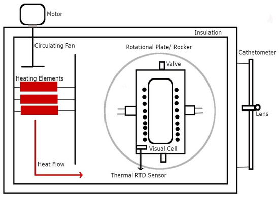
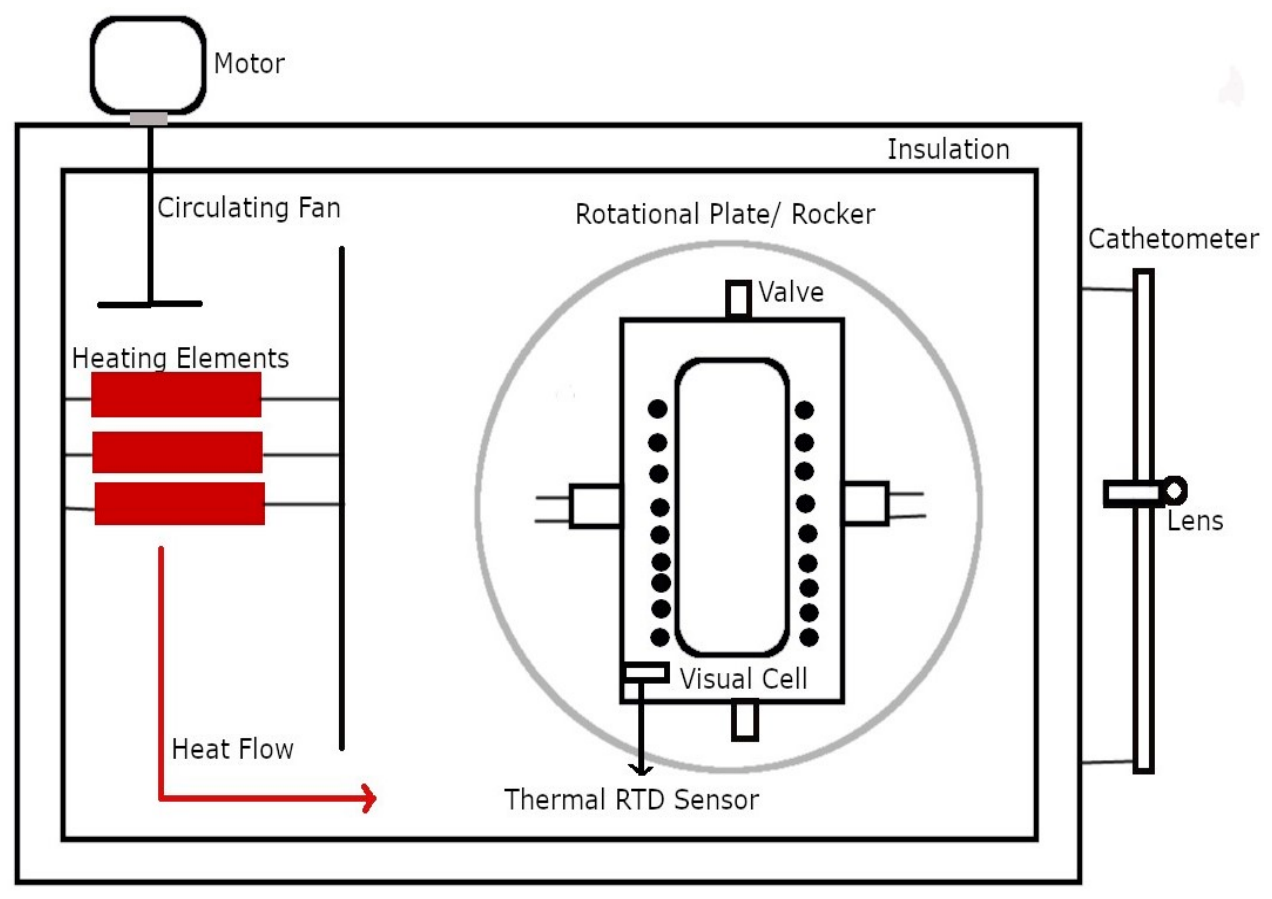
- Schematic and design: A PVT cell was utilized to replicate the behavior of the prepared samples under reservoir conditions in order to assess the impact of an increase in temperature and pressure on the prepared seawater and aquifer samples. Figure 1 is an image which shows the PVT cell’s schematic.
Figure 1.
PVT cell schematic.
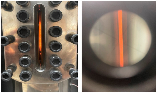
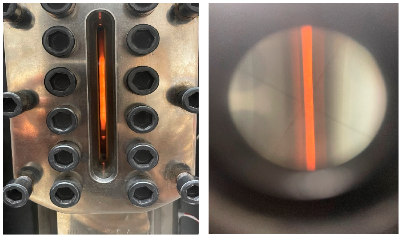
A mounted rocker that facilitates visual inspection of the contents loaded into the cell is part of the configuration. The rocker’s design allowed for both manual and remote control and operation. The hand wheel on the side of the machine allows users to rotate the rocker manually and remotely from the software program when connected to the computer. Fluid examination is made possible by the high-pressure–high-temperature (HPHT) visual cell. Any user can see the phase behavior of the fluids inside the cell at various temperature and pressure values due to its two pieces of sapphire glass. The high-pressure–high-temperature visual cell is ideal for a variety of studies needing extremely high-pressure ranges, since it can tolerate pressure as high as 10,000 psi. The cell’s chamber has a total fluid capacity of roughly 200 cc. The PVT cell’s revolving fan aids in dispersing the heat produced by the heating components. The cell’s temperature is recorded by the thermal RTD (Resistance Temperature Detector) sensor at all times. The heat produced in the cell is retained by the insulation surrounding the design. With the use of a mirror linked to the cell, the cathetometer’s telescope enables the user to securely see the contents of the cell.
- Pump: The model 500D Teledyne Isco Pump was utilized. The pump’s highest-pressure rating is approximately 3750 psi, and its volume capacity is approximately 500 cc. The user is able to control the desired pump operation specification using the pump display. Parameters like pressure and flowrate can be adjusted to the appropriate values based on the needs of the experiment.
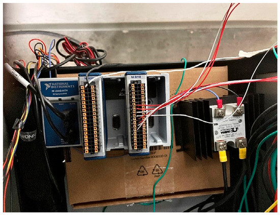
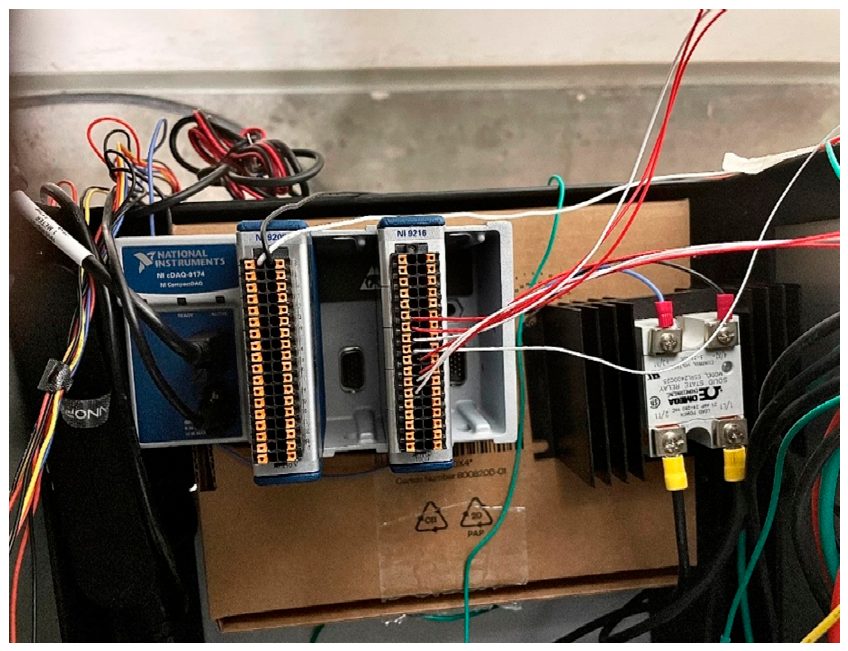
- Data Acquisition: Data Acquisition (DAQ) and a computer application (LABVIEW) are needed to remotely control the PVT cell. The DAQ is connected to the temperature sensor of the PVT cell as well as to the computer via a USB. The signals that a DAQ receives from the sensor are processed, converted, and transmitted to a computer for display. The DAQ used is shown in Figure 2 below.
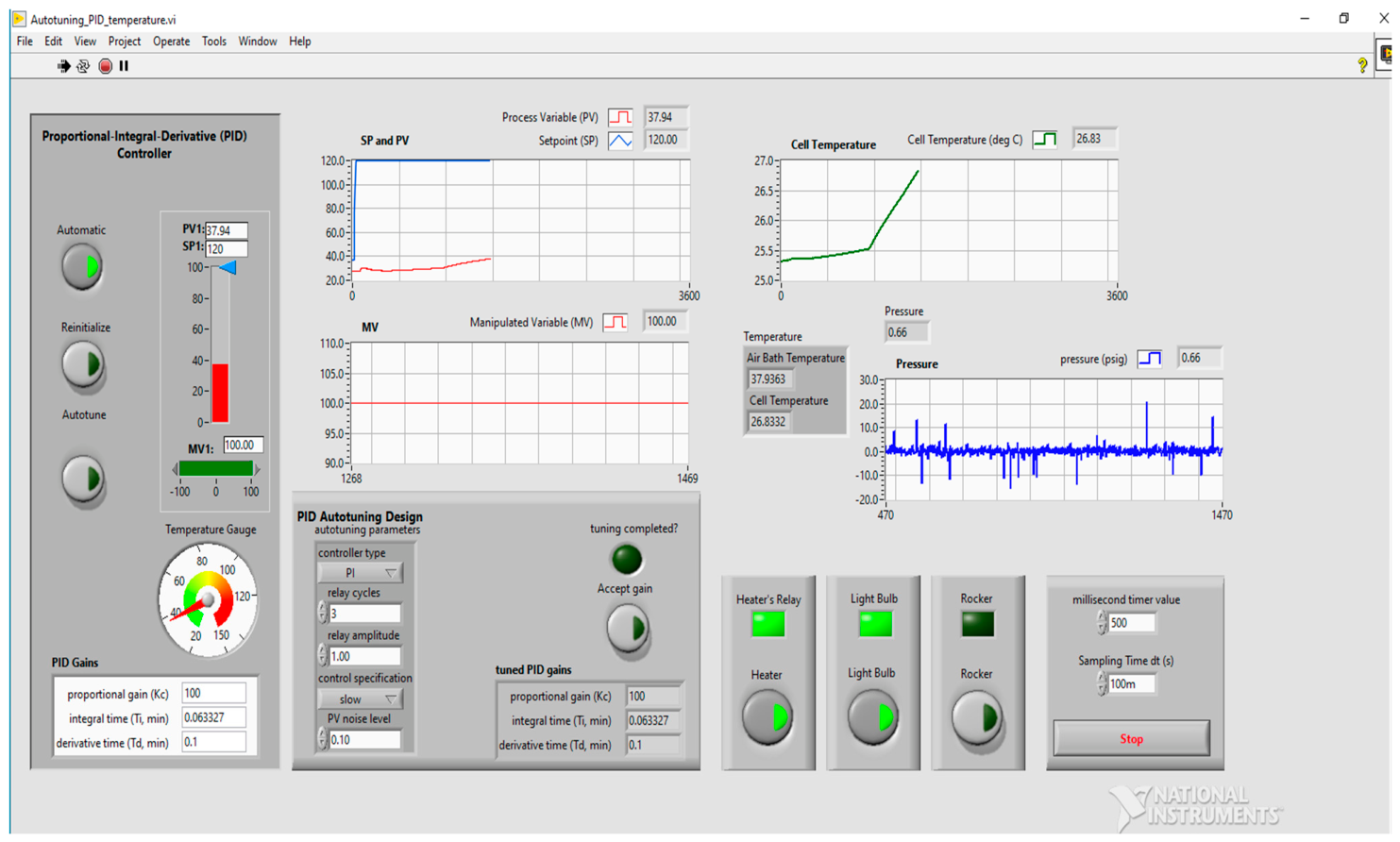
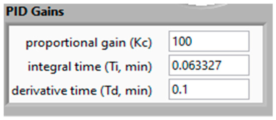
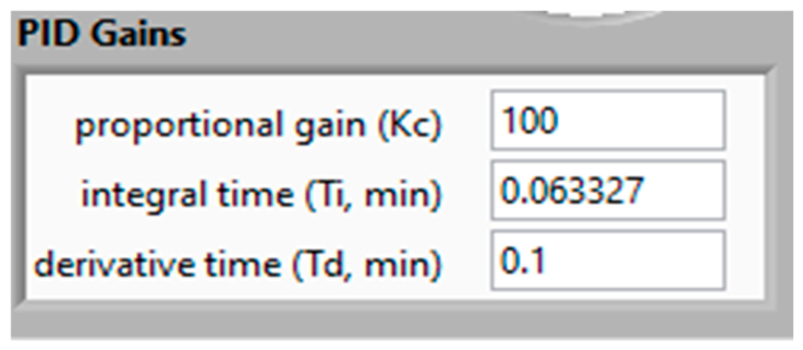
- Computer software: A computer application called LABVIEW was utilized to assist in remotely controlling the various parts of the cell. The user could operate the rocker, the heating, and the lightbulb within the cell from the computer. Additionally, the computer program may interact with DAQ to graphically display metrics like temperature and pressure. Because of this, the application is highly useful for monitoring experiments and managing equipment during an experiment. The computer software program has to set PID (proportional integral derivative) gains, which are crucial to controlling the heater. To prevent erratic temperature swings, these parameters have to be set before the heater is turned on. The figure below shows the ideal PID values that were found after a number of tests, but with an absolute inaccuracy of roughly 0.1 °F. The LABVIEW computer program is depicted in Figure 3 and Figure 4 below.
Figure 2.
Image of the Data Acquisition (DAQ) device.
Figure 3.
Interface of the LABVIEW computer program.
Figure 4.
Image showing optimum PID gains for the LABVIEW computer program.
2.8. Core Flooding
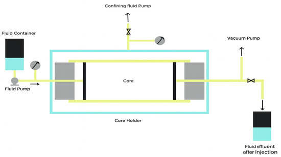
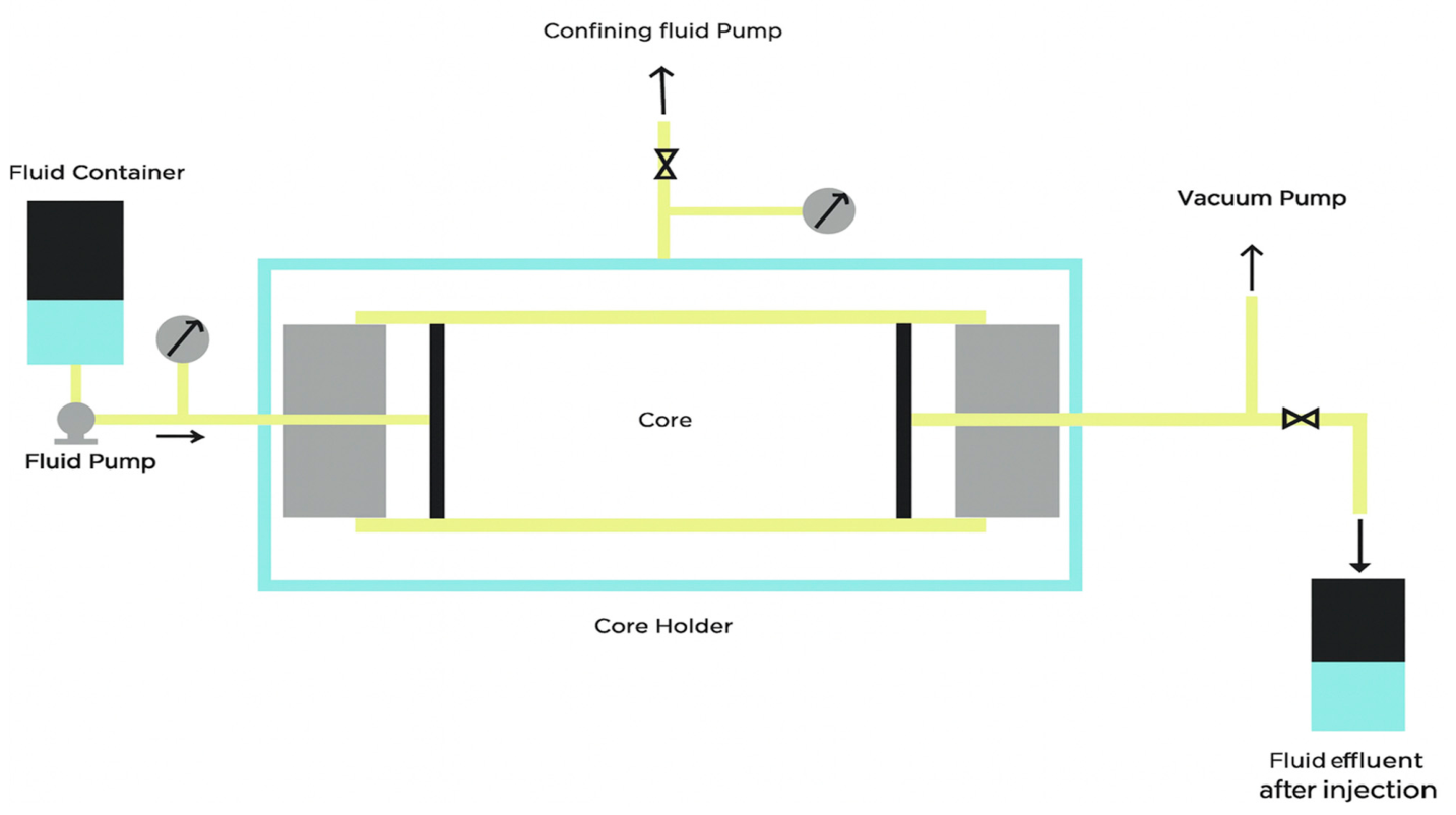
One crucial reservoir characteristic is permeability. To make better decisions about oil and gas recovery, reservoir engineers must be able to calculate permeability. Two conditions are typically used for core flooding: either a constant flowrate through the core sample or constant pressure across the core sample. When utilizing a mathematical model to analyze the experimental results, these two approaches are highly practical. Figure 5 shows a schematic of the core flooding setup.
Figure 5.
Schematic of core flooding setup.
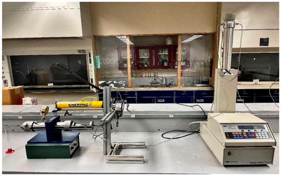
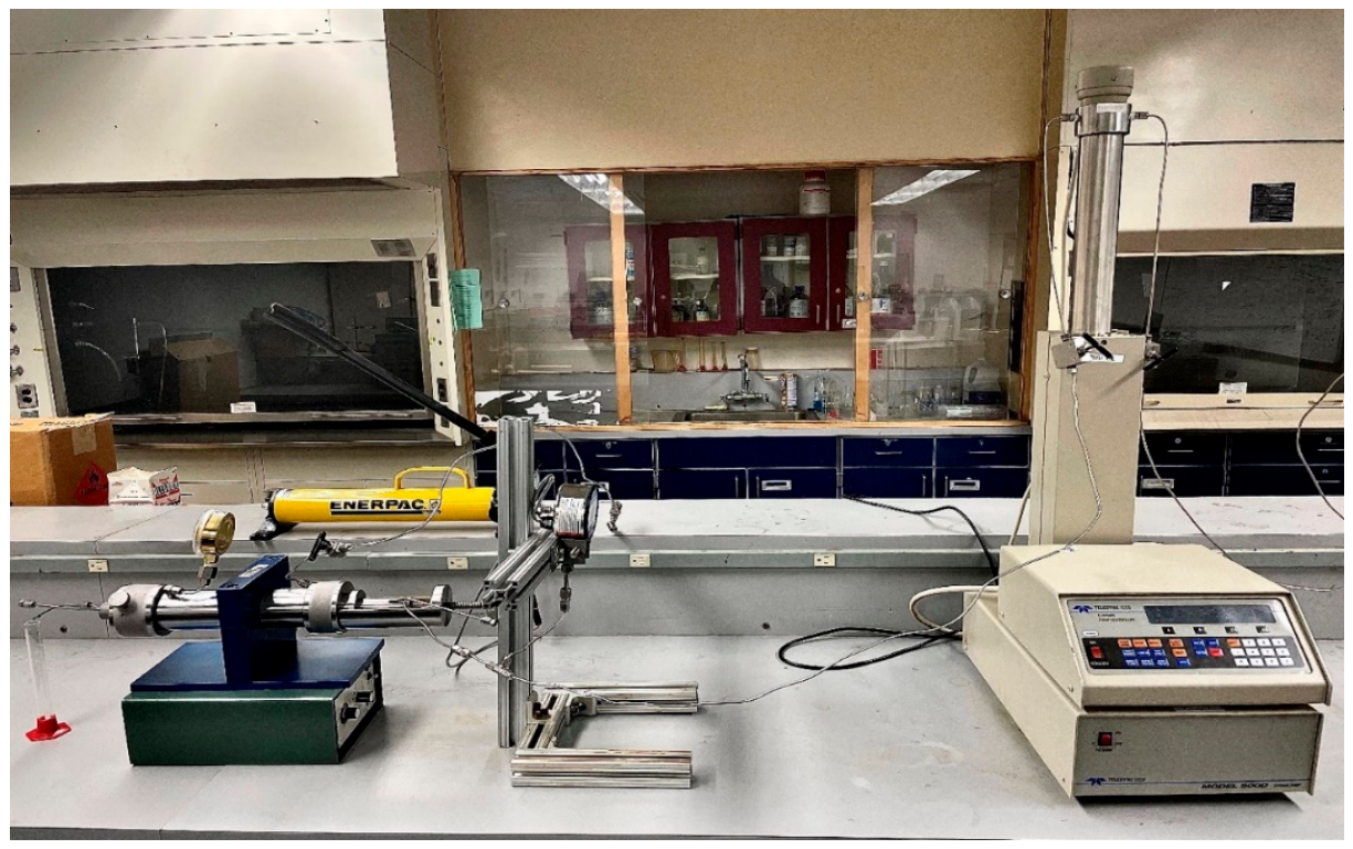
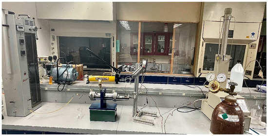
A core flooding experiment was carried out to ascertain how scale precipitation affected permeability. The permeability of a Berea sandstone core was investigated in this experiment. Following the development of scale due to the injection of seawater and aquifer water, permeability was further assessed. Figure 6 below shows the setup and equipment used:
Figure 6.
Image of core flooding setup.
- The core holder: The core sample is kept in the core holder. The core is housed in a sleeve inside the core holder. A core can be inserted and removed from the two open ends of the sleeve and core holder. The outer and inner diameters of the cylindrical core holder are approximately 2.44 inches and 1 inch, respectively. Additionally, the core holder is roughly 17 inches long. The core holder can withstand temperature of up to 3000 degrees Fahrenheit and pressure of up to 5000 psi. A pressure gauge that is linked to the core holder aids in monitoring the amount of overburden pressure applied to the core at any time.
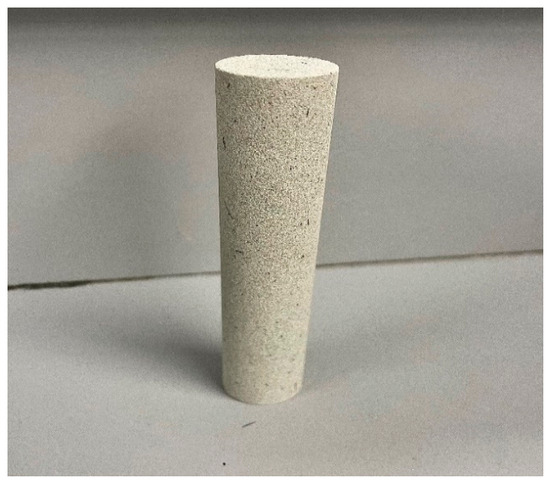
- The Berea sandstone core: The core sample employed in this study was Berea sandstone. The length of the core was measured to be 6 inches using a pair of vernier calipers. The cross-sectional area was also measured to be 1 inch. It was ensured that the core was vacuumed before use to remove air bubbles and also any fine grains which may have bridged the pores of the core. The Berea sandstone core has very good permeability; hence any decrease in permeability due to the effects of scale precipitation would be clearly noticed. An image of the Berea sandstone core is shown in Figure 7.
- Overburden pressure pump: Overburden pressure was created around the core using the ENERPAC P80, Two Speed, ULTIMA steel hydraulic hand pump. The maximum operational pressure rating for this pump is 10,000 psi. The gadget’s quick grasp handle makes it easier to carry around. The device is 7.65 inches tall and 23.5 inches long. The handle is used to operate the pump. The overburden pressure is created when the handle is dropped because the motor oil surrounds the core sample in the sleeve through the connecting lines.
- Overburden pressure gauge and pressure gauge: The overburden pressure created inside the core holder as a result of the overburden pressure pump’s operation is measured by a pressure gauge that is attached to the core holder. Up to 400 psi, or 2800 kPa, of pressure can be measured using this gauge. Between the core holder and the 500D syringe Teledyne ISCO pump is another pressure gauge. This pressure gauge’s presence aids in precisely determining the pressure at the point when the ISCO pump and core holder experience pressure changes. This gauge can measure pressure up to 1000 psi and has a full-scale accuracy of 0.25%.
- 500D syringe Teledyne ISCO pump: Seawater and aquifer water were injected using the Teledyne ISCO 500D syringe pump. With flowrates ranging from 0.001 cc/min to 204 cc/min, the pump has a capacity of roughly 500 cc. Up to 3750 psi of pressure is supported by the pump. The pump has a controller that lets the user adjust the flowrate and pressure.
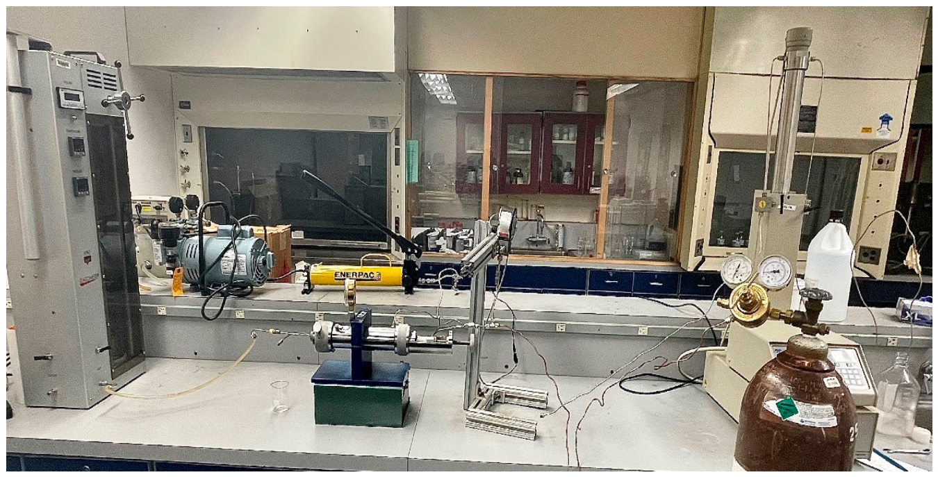
- Manual gasometer: A manual gasometer is intended to measure gas volumes at room temperature and pressure. The apparatus is made to measure precise gas volumes of up to 4000 cc. In this study, a Berea sandstone core’s permeability was measured using a gasometer. Gas quantities at a specific pressure can be measured using the gasometer. Control valves, a floating piston, a crank, a temperature probe, a pressure sensor, and a glass tube are all part of the arrangement. The main purpose of this device’s design is to monitor gas volume in ambient circumstances. The core permeability measurements were conducted using non-flammable helium gas. Figure 8 shows the core flooding setup with the manual gasometer connected.
Figure 7.
Image showing the Berea sandstone core.
Figure 8.
Image of manual gasometer connected to the core flooding setup.
2.9. Core Cleaning
The permeability and porosity measurements of core samples may be impacted if they come into contact with the drilling mud while being extracted from a well. Additionally, natural reservoir fluids including oil, brine, and heavy residue may be present in the core pores.
Therefore, it is essential to fully eliminate the original fluids that were initially present in the core sample before performing the majority of laboratory analyses. Solvents are typically used in the core cleaning process by flushing, flowing, or coming into contact with the fluids that initially saturate the core. Depending on the application and kind of core, different solvents are needed. While toluene has also been proven to be quite effective when used for asphaltic crudes, chloroform has been discovered to yield very good outcomes when utilized in several North American crudes. We employed two different kinds of solvents in our situation. Methanol was injected to clean the core after first injecting tetrahydrofuran, which has a boiling point of 65 °C. It should be mentioned that tetrahydrofuran is a potent solvent that can dissolve petroleum heavy ends, water, oil, and salt. Solvent flushing (direct pressure) with a core flood setup is how core cleaning is accomplished. Before injecting the solvent, care should be taken to ensure that the core is vacuumed. The effectiveness of cleaning is decreased when air or gas is present in the pores. The size of the core and the amounts of hydrocarbons in the sample typically determines how much solvent is needed for core cleaning. We did not establish a cap on the amount of solvent that may be injected, and when the effluent is clean, the core was deemed clean. It is necessary to dry each core sample until the weight stabilizes. Although drying periods might vary greatly, they are typically more than four hours. The apparatus used in the core cleaning process includes the following:
- 500D syringe Teledyne ISCO pump: Solvents were injected through the core sample using the Teledyne Isco Pump. The injection rate was permitted to fluctuate, while a pressure of 200 psi was specified. When the effluent at the core holder’s output was clear, solvent injection was terminated.
- GAST compressor vacuum pump: The core sample’s potential air pockets were eliminated using the GAST compressor vacuum pump. A rubber tube was used to connect the vacuum pump to the core holder outlet once the core sample had been put into the core holder. The core was vacuumed using the vacuum pump until the opposite end of the core holder, which had a pressure gauge affixed, could feel the pressure effects.
- OFITE roller oven: The core samples were dried using the OFITE roller oven. The type of rock and amount of clay determine the oven temperature. This roller oven was chosen because any sample put inside would be continuously moving to guarantee that the heat was distributed evenly across the sample. It is also possible to operate the OFITE roller oven at temperature as high as 232 °C. During preparation, clay-containing samples must not be dehydrated. In order to avoid the dehydration of clays, we attempted to adopt a minimum temperature of 65 °C. Until the sample weight stayed constant over time, the weight was measured on a regular basis (every hour).
2.10. Core Porosity Calculation
The dry and saturated weight of the Berea sandstone core have to be ascertained in order to calculate its porosity. Brine was the saturation fluid. An electronic scale was used to determine the dry core sample’s weight. The core was saturated with brine after being put in the core holder. An electronic balance was also used to determine the saturated weight of the Berea sandstone core. The core’s diameter and length were measured using a vernier caliper. The porosity of the core sample was then computed using the formulas below.
where:
- = Weight of the core saturated with brine.
- = Dry weight of the core.
- = Density of brine.
The cross-sectional area of the core was calculated using the equation
After the pore volume was calculated, the core porosity was calculated using the equation
where:
- = Pore Volume.
- = Bulk Volume.
2.11. Absolute Permeability Calculation
- Liquid as the flowing fluid: The ease with which a fluid passes through a porous medium when the rock or porous medium is saturated with a single fluid is known as absolute permeability. The unit of absolute permeability is Darcy, where 1000 MD is equal to 1 Darcy. The most popular method for determining absolute permeability is to flood a core sample in the lab with a single-phase fluid, such as gas, oil, or brine, until a steady state flow condition is reached. Determining core permeability entails setting constant pressure while allowing flowrates to fluctuate. A comparable flowrate at a given differential pressure was computed using the cumulative volume injected over time. The core’s absolute permeability was determined using the Darcy equation.where:
- Flowrate in cc/min.
- = permeability in md.
- cross sectional area in cm2.
- = viscosity of the injected fluid in cp.
- = Length of core in cm.
- = Differential pressure in psi.
- = Permeability of core in md.
The core permeability can be determined when the viscosity of brine, the length of the core and the cross-sectional area of the core are known.
- Gas as the flowing fluid: Permeability is a quality that depends on the rock rather than the kind of fluid used to assess it. In the event of a non-reactive liquid, this statement is accurate. When gas was employed as the fluid, Klinkenberg discovered that the permeability measurements were not consistent and that the results changed according to the type of gas used. Helium gas was utilized as the flowing fluid in this investigation. A manual gasometer was attached to the core flooding setup in order to measure the gas volume over time at various upstream pressure values. The Darcy equation for gas was then used to compute gas permeability, taking into account a linear and horizontal flow at pressure below 2000 psia. The following formula can be used to determine a gas’s permeability when the area, length, compressibility factor, and viscosity of the gas are known.where:
- = Gas flowrate in SCF/d.
- = Standard temperature in Rankine.
- = Gas relative permeability.
- = Permeability in md.
- = Area in ft2.
- = Standard pressure in psia.
- = Temperature in Rankine.
- = compressibility factor.
- = gas viscosity in cp.
- = length in ft.
- = Pressure in psia.
2.12. Scaling Effect on Berea Sandstone Core Permeability
Determining the impact of scale precipitation on the Berea sandstone core came next, following the determination of the core’s absolute permeability. The process that was carried out is explained below. To prevent any possible scale formation from impacting equipment and obstructing the connection lines, all connections and equipment were cleaned with distilled water.
The following experimental conditions were applied:
- Injection flowrate: 0.5 cc/min (constant rate mode using Teledyne ISCO 500D syringe pump).
- Injection pressure: Upstream pressure varied between 50 and 100 psi (differential pressure across core).
- Temperature: Ambient (24 °C) for scaling experiment.
- Pore volumes injected: 3 PV of aquifer water, followed by 1 PV of seawater.
3. Results
3.1. Prepared Seawater and Aquifer Water Samples
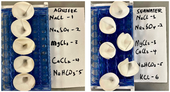
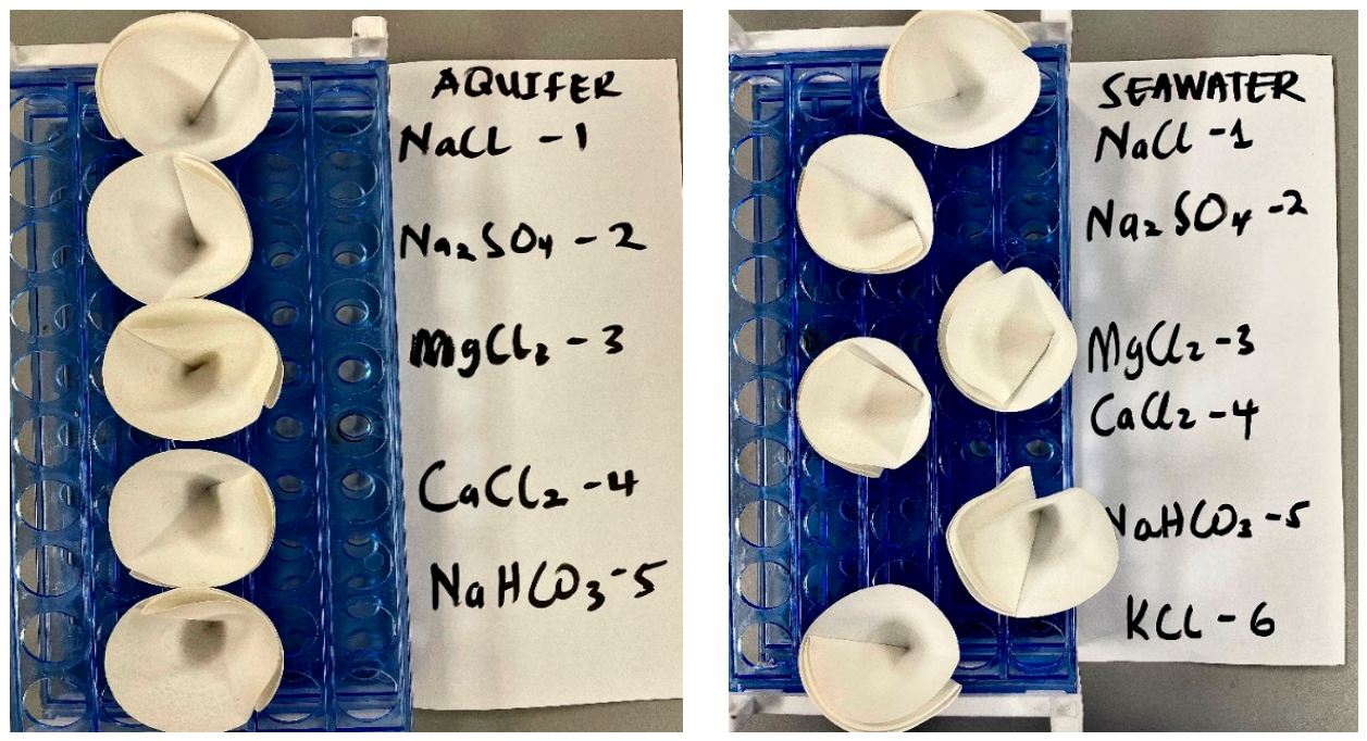
Salts were added one after the other to seawater and aquifer water samples, and the mixture was then filtered. The outcomes of filtering the seawater and aquifer water samples at each stage are displayed in the table. After a 200 cc sample of seawater and aquifer water was prepared, the percentages of total undissolved salt in the aquifer water and seawater samples were 2.8% and 2.14%, respectively. Table 3 and Figure 9 below provides a summary of the sample preparation and a pictorial view of the filter paper after the samples were filtered. This section presents the results of the conducted experiments following procedures previously described in [1].
Table 3.
Preparation of seawater and aquifer water samples.
Figure 9.
Filter paper samples of the prepared solutions were filtered.
3.2. Turbidity
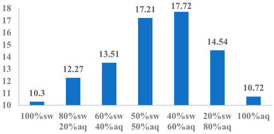
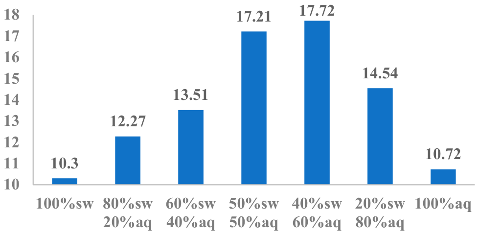
Using the experimental results shown below in Figure 10, the turbidity of the various ratios of the seawater and aquifer water samples in 15 mL conical centrifuge tubes was measured.
Figure 10.
Chart of turbidity for different ratios of SW and AQ water samples.
3.3. Salinity
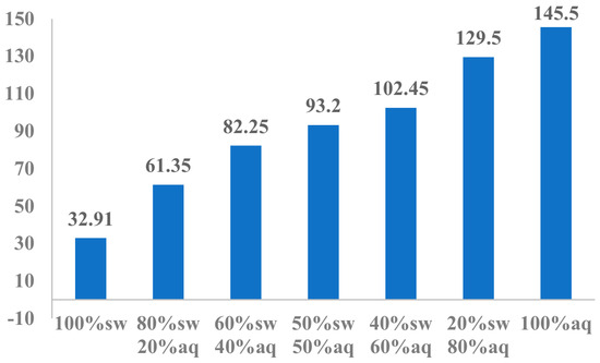
Since the vernier salinity probe used in the measurement could only cover a salinity range between 0 and roughly 50 ppt, samples were diluted prior to measurement. With the exception of the initial measurement for a sample with a 100% seawater concentration, all subsequent samples were diluted and multiplied by a dilution factor of five in order to recover the initial sample concentration. The salinity data for the various mixed seawater and aquifer water ratios are displayed in Table 4.
Table 4.
Salinity for different ratios of SW and AQ water samples.
The salinity for the different ratios of the seawater and aquifer solutions is displayed in Figure 11 below.
Figure 11.
Chart of salinity for different ratios of SW and AQ water samples.
3.4. pH
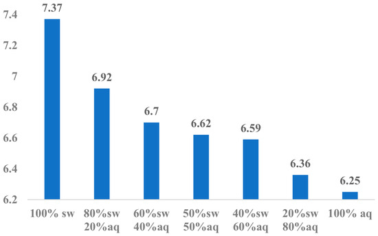
The prepared seawater and aquifer water samples were tested for pH. The solutions’ pH values varied from 7.37 to 6.25, as shown in Figure 12.
Figure 12.
Chart of pH for different ratios of SW and AQ water samples.
3.5. Zeta Potential
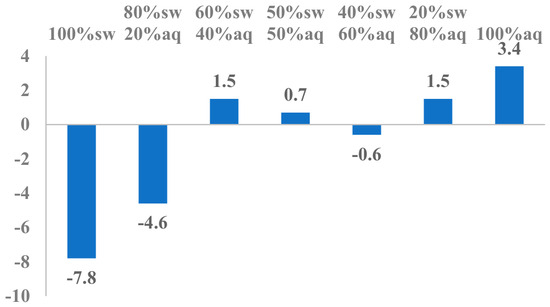
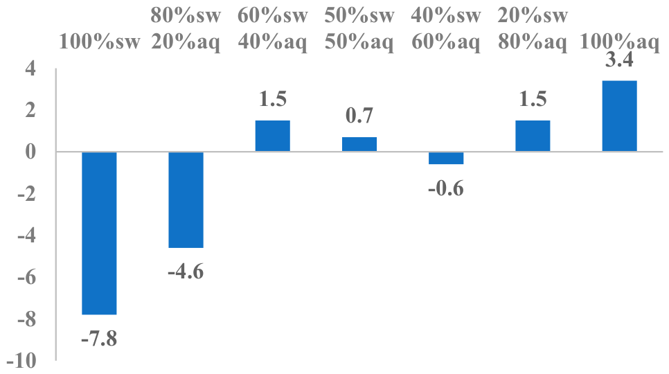
The stability of the various seawater and aquifer water samples, as well as the solution’s surface charge, was assessed using zeta potential tests. The zeta potential measurement findings for each of the examined solutions are listed below in Figure 13.
Figure 13.
Chart of zeta potential for different ratios of SW and AQ water samples.
3.6. Stability of the Prepared Aquifer Water Sample Using PHREEQC Software
The tendency or potential of the produced solutions’ self-precipitating was assessed using PHREEQC (version 3) with the phreeqc.dat database, for the reported compositions of the seawater and aquifer water samples. The column labeled “SI” in the table below represents the saturation index, where SI > 0 means supersaturation (precipitation is thermodynamically favorable), SI = 0 means equilibrium, and SI < 0 means undersaturation (no precipitation is expected). This is followed by a column labeled “log IAP” for the log of the ion activity product and “log K” for the solubility constant. The chemical formulas for each of the compounds are listed in the final column. Table 5 and Table 6 show a summary of the results.
Table 5.
Saturation indices of the seawater sample.
Table 6.
Saturation indices of the aquifer water sample.
The sample of seawater contained the carbonate minerals aragonite (SI = 0.54), calcite (SI = 0.69), and dolomite (SI = 2.17) in a supersaturated state, which means that such minerals are thermodynamically capable of precipitating. However, the sample was found to be lacking in anhydrite (SI = −0.9), gypsum (SI = −0.6), halite (SI = −2.33), and sylvite (SI = −3.47), which implies that the precipitation of sulfate and chloride salts is not possible from seawater alone. The positive SI values of the carbonate phase show that the concentrations of Ca2+ and carbonate ions are above the solubility limits, thus making the initiation of carbonate scaling quite easy.
The aquifer water sample showed a much greater level of supersaturation than seawater for all carbonate phases: aragonite (SI = 1.68), calcite (SI = 1.83), dolomite (SI = 2.88), and siderite (SI = 0.16). The positive numbers suggest that there is a strong thermodynamic potential for carbonate precipitation. Halite (SI = −0.96) was still a little undersaturated, which means that no NaCl precipitation is expected.
Compared with seawater, aquifer water in general had about two or three times the SI values for calcite and aragonite, while the dolomite SI was around 30% higher, which is consistent with its higher ionic strength and ion concentrations.
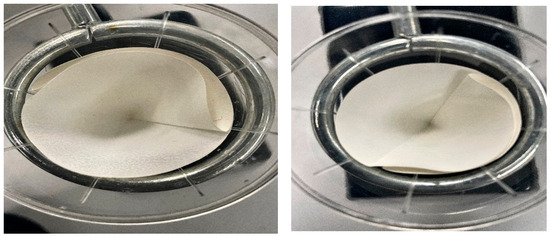
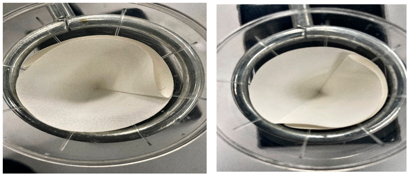
Two weeks after they were created, 100-milliliter aquifer and seawater samples were filtered. The filter paper weighed 0.558 g at first. The final filter paper weight was 0.776 g for the aquifer water sample and 0.574 g for the seawater sample. The samples were then filtered and oven-dried. An image of filter paper for both after the samples were filtered can be found in Figure 14 below.
Figure 14.
Filter paper after 100 mL aquifer water solution (on the left) and seawater (on the right) were filtered.
3.7. Scaling Test Under Standard Conditions
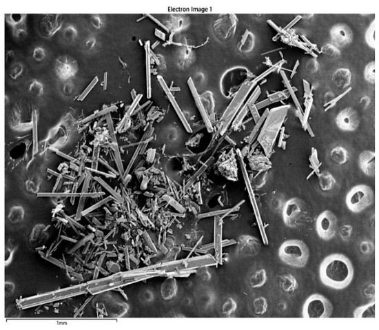
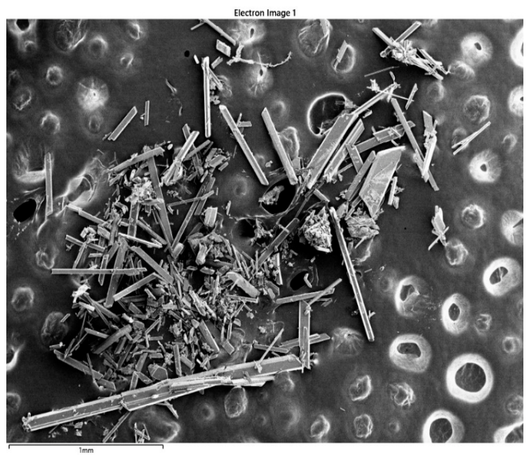
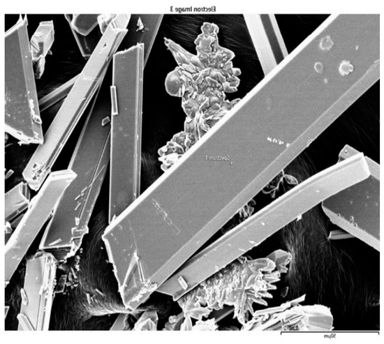
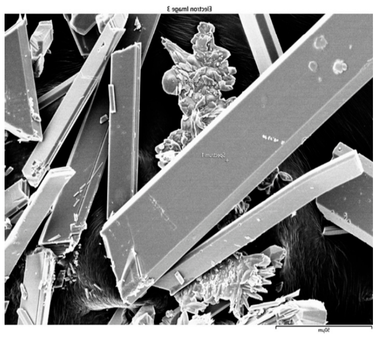
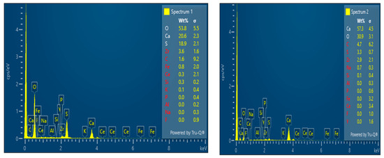
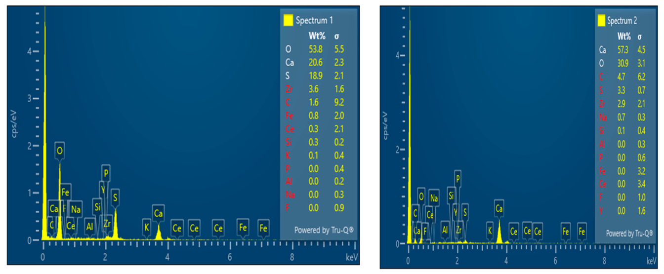
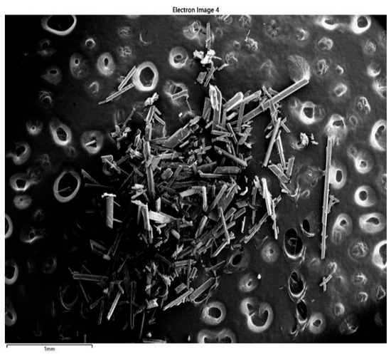
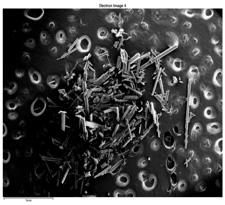
In order to examine the precipitation of scale, samples of aquifer water and seawater were combined in equal proportions. SEM (scanning electron microscopy) and EDS (energy-dispersive X-ray spectroscopy) studies were carried out in order to assess the shape and content of the resulting precipitation. The examination of two zones (Zone A and Zone B) on filter paper following the filtering of seawater and aquifer water samples is displayed. Figure 15, Figure 16 and Figure 17 below show the analysis results for zone A and Figure 18, Figure 19 and Figure 20 for zone B.
Figure 15.
SEM image of Zone A.
Figure 16.
Detailed SEM image of Zone A.
Figure 17.
Element analysis of Zone A.
Figure 18.
SEM image of Zone B.
Figure 19.
Detailed SEM image of Zone B.
Figure 20.
Element analysis of Zone B.
3.8. Scaling Test Under Reservoir Conditions
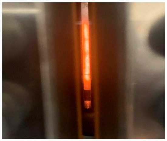
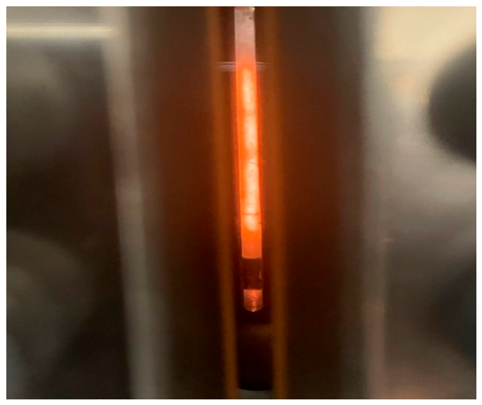
A PVT cell with a temperature of 125 °C and a pressure of 1000 psia was used to conduct a scaling study under reservoir conditions. Using a pump, a 105 mL volume of aquifer water sample was initially pumped into the cell, followed by 105 mL of seawater solution. The two mixtures were then left to stand for approximately 120 h. The timeline of the PVT cell experiment was as follows: (1) First, at t = 0 h, 105 mL of aquifer water was injected; immediately after, 105 mL of seawater was injected. (2) The cell was then sealed and heated/pressurized to 125 °C and 1000 psia within 2 h. (3) The mixture was kept under these conditions for 120 h (5 days). (4) After 120 h, the cell was cooled and depressurized, and the contents were recovered. The samples can be seen through the sapphire glass of the PVT cell in the image below both before and after the analysis was finished after five days. After the recovered samples from the PVT cell were filtered, the weight of the filter paper was noted. Equivalent volumes of 50% seawater and 50% aquifer water samples were mixed. Figure 21 and Figure 22 show the sample right after its injection into the PVT cell and the sample after 120 h. Table 7 below displays the results.
Figure 21.
Seawater and aquifer water sample after their injection into PVT cell.
Figure 22.
Seawater and aquifer water sample after 120 h.
Table 7.
Filter paper weights after temperature and pressure effect.
Under ambient conditions, the mixture of 100 mL of seawater and 100 mL of aquifer water yielded 0.243 g of precipitate; in contrast, under reservoir conditions (125 °C, 1000 psia), the same mixture yielded 0.140 g of precipitate which is 42% less than the previous precipitate mass. The main reason for this reduction is the increase in temperature and pressure.
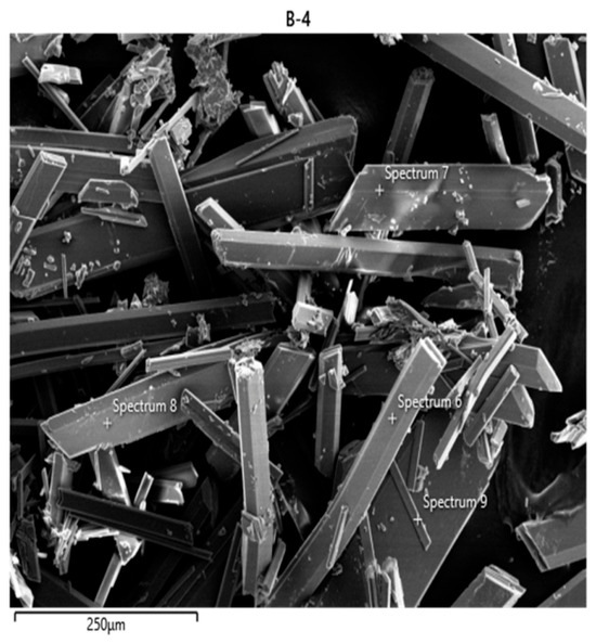
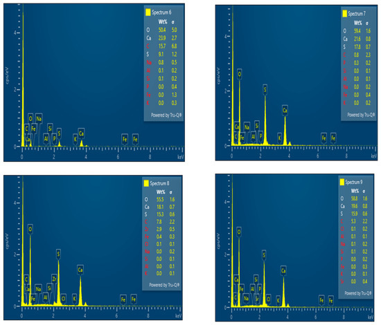
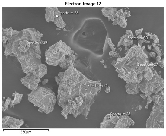
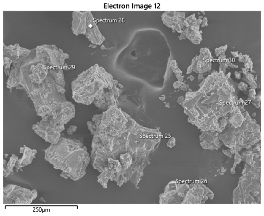
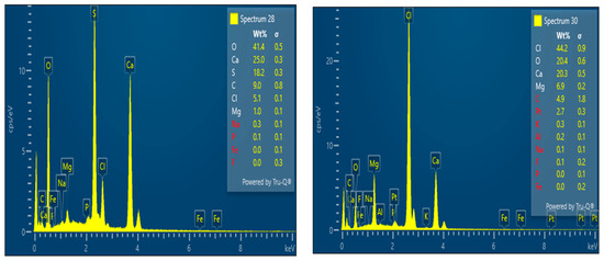
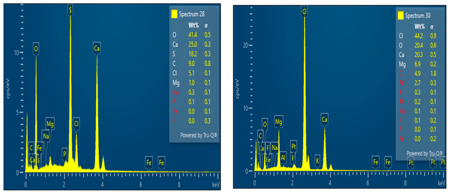
Following the recovery and filtering of the samples, the filter paper was brought to the laboratory for examination of the content and of the form of the ensuing scale precipitate. Figure 23 and Figure 24 shows the results of seawater and aquifer water sample after the increase in temperature and pressure.
Figure 23.
Electron image of seawater and aquifer water sample after effect of temperature and pressure.
Figure 24.
Element analysis of precipitate after temperature and pressure effects using the PVT cell.
3.9. Determination of Core Properties
Table 8 below present a summary of the properties of the Berea sandstone core utilized in this study.
Table 8.
Summary of Berea sandstone core properties.
3.10. Absolute Permeability Determination Using Liquid with a Constant Pressure Specified for the Berea Sandstone Core
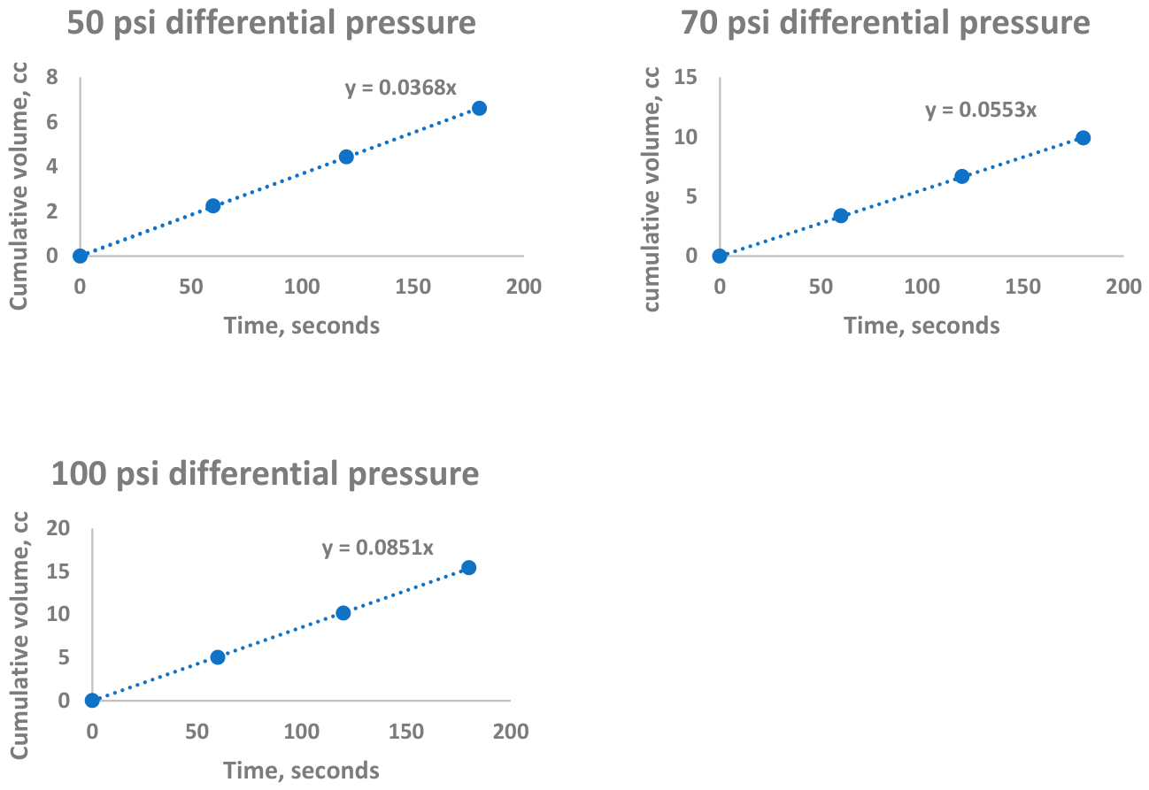
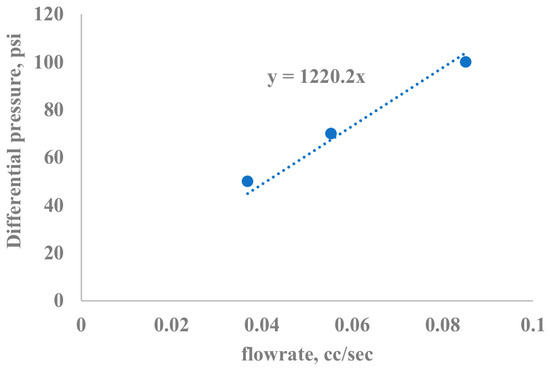
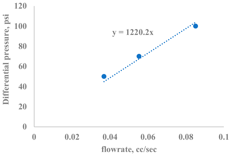
The data displayed are an overview of the findings from cumulative volume versus time charts at various differential pressure values. Details are provided in Appendix A. The flowrates at the different differential pressure values were determined from the results. Table 9 and Figure 25 show a summary of the findings.
Table 9.
Table of flowrate and differential pressure.
Figure 25.
Chart of differential pressure versus flowrate.
The absolute permeability was calculated to be 37.32 md.
3.11. Absolute Permeability Determination Using Gas with Constant Pressure Specified for the Berea Sandstone Core
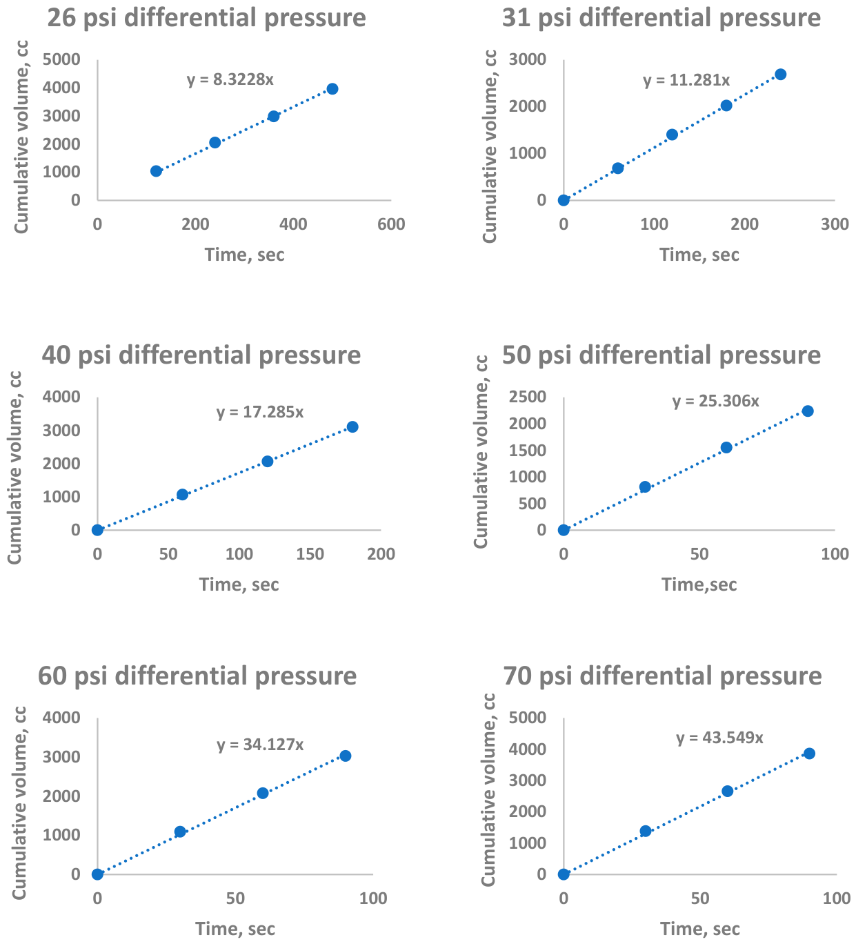
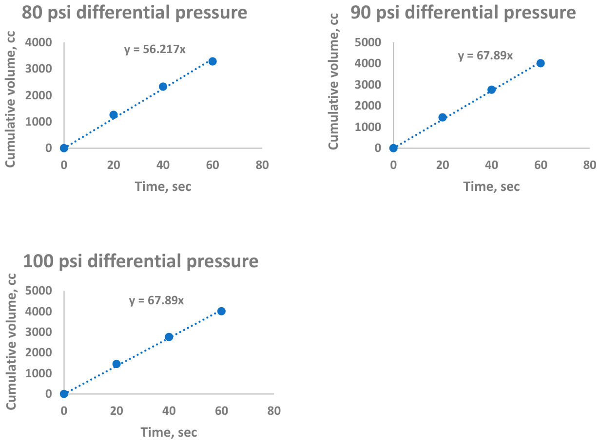
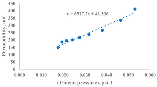
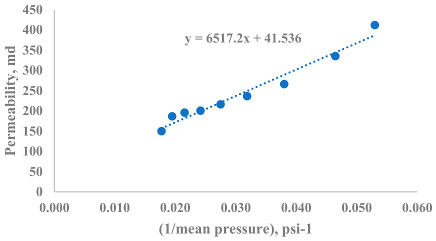
The data displayed in Table 10 and Figure 26 are an overview of the findings from cumulative volume versus time charts at various differential pressure settings. Details are provided in Appendix A. The flowrates at the different differential pressure values were determined from the results.
Table 10.
Permeability versus inverse of mean pressure.
Figure 26.
Chart of permeability versus inverse of mean pressure.
The intercept for the plot of permeability against the inverse of mean pressure can be used to get the absolute permeability value using gas as the flowing fluid. The plot reveals that the Berea sandstone core’s permeability was 41.536 md.
3.12. Permeability After Scale Formation for the Berea Sandstone Core
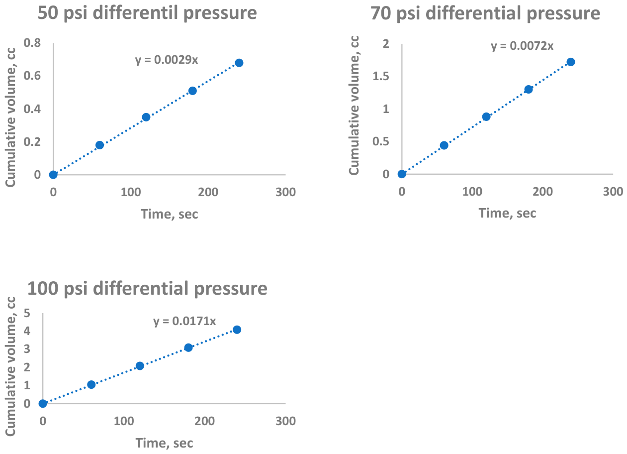
The data displayed are an overview of the findings from cumulative volume versus time charts at various differential pressure settings. Appendix A contains more information. The results produced were used to calculate the flowrates at the various differential pressure values. Table 11 and Figure 27 show a summary of the results.
Table 11.
Flowrate and differential pressure.
Figure 27.
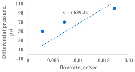
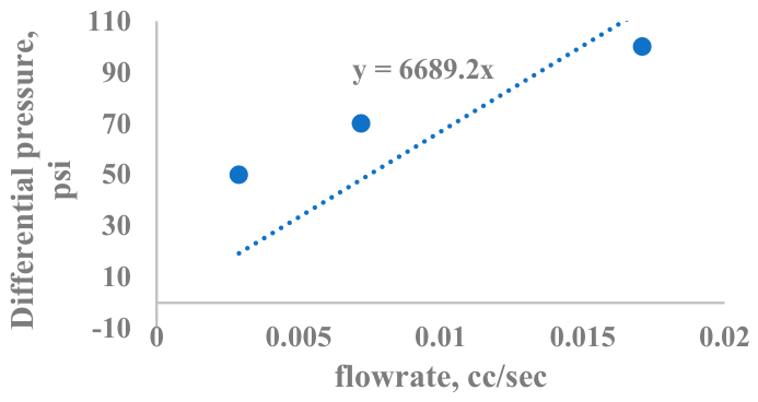
Graph of differential pressure vs. flowrate.
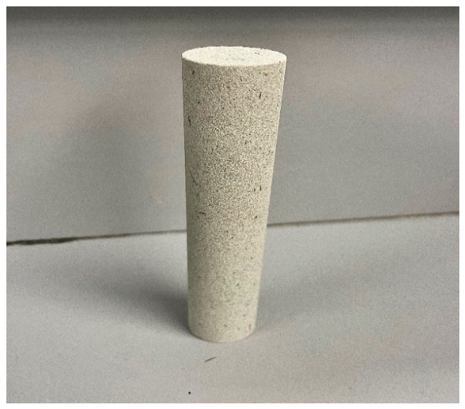
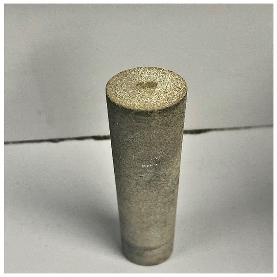
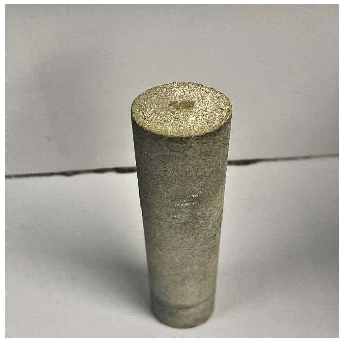
The permeability of the sandstone core, which was measured after the setup was left for five days, was found to be 6.94 md after infusing 3 PV of aquifer water and then 1 PV of seawater. Figure 28 shows an image of the Berea sandstone core sample. Table 12 below shows a quantitative comparison of Berea sandstone core permeability before and after scale formation.
Figure 28.
Image of Berea sandstone core after scale formation.
Table 12.
Quantitative comparison of Berea sandstone core permeability before and after scale formation.
Following scale precipitation, the absolute permeability of the Berea sandstone core dropped from 37.32 to 6.94 md, which is equivalent to an 81.4% reduction in permeability. The scale deposits blocked the major part of the pore throats and flow pathways of the core sample.
The permeability reduction of 81.4% aligns well with the turbidity and scale mass data, both indicating the highest level of scale formation in the 40% SW/60% AQ mixing ratio. Such a high permeability decline indicates that apart from scale of carbonate and sulfate being formed in the bulk solution, these also got deposited inside the pores of the porous medium, especially at the pore constrictions.
4. Discussion
Water becomes less clear as its turbidity rises, and turbidity measurements indicate how cloudy a liquid is. Tests for turbidity show whether a given solution is compatible [2,5]. The results show that when 40% of the seawater and 60% of the aquifer water samples were combined, the highest turbidity was seen. Additionally, samples of seawater and aquifer water in 100% ratios showed the lowest turbidity.
In general, the concentration of salts in a solution is referred to as its saltiness. The enhancement of oil recovery from a reservoir is significantly influenced by the salinity of a solution. The findings of the experiment verify that the resulting salinity showed an increasing trend with the increase in aquifer water content.
The concentration of H+ rises when a solution’s pH falls. In general, samples with comparatively higher seawater contents had higher pH. The 100% aquifer water sample had the lowest pH [12].
The 42% decrease in precipitate mass under reservoir conditions (125 °C, 1000 psia) relative to ambient conditions, as reported, is based on a number of thermodynamic changes. For carbonate minerals (CaCO3), solubility typically decreases with the increase in temperature [6]. Nevertheless, at high temperature, formations of soluble ion pairs, e.g., CaHCO3+ and MgHCO3+, are thermodynamically favored, effectively removing the Ca2+ and Mg2+ ions from carbonate precipitation. Pressure changes result in two very important consequences. Firstly, more CO2 is held in solution at higher pressure, which changes the equilibrium and results in pH lowering (acidification), thus increasing carbonate mineral solubility [12]. Secondly, the molar volume change for CaCO3 dissolution is positive; thus, increasing pressure favors dissolution more than precipitation. The net result at 1000 psia and 125 °C is greater carbonate solubility than that under ambient conditions even though carbonate minerals experience a retrograde temperature effect. As for sulfate minerals (e.g., gypsum and anhydrite), pressure effects compensate for the decrease in solubility with temperature, leading to overall less precipitation [10].
From the turbidity and precipitation mass results, major scale formation was identified in the 40% SW/60% AQ mixing ratio, and the permeability drop of 81.4% is a solid confirmation of this. The turbidity tests revealed that the 40% SW/60% AQ mixture is the one that would most likely result in scaling. However, the PVT experiment with the cell had to be done with a 50%/50% mixture due to experimental limitations. Hence, the lowered mass of precipitate shown from 0.243 g (ambient, 50/50) to 0.140 g (125 °C, 1000 psia, 50/50) is the temperature and pressure influence for that proportion only. Since the permeability decline was quite high, this indicates that carbonate and sulfate scale was not only generated in the bulk solution but also led to deposition in the porous medium, especially at the pore constrictions [2,11].
The mixed solutions reached a zeta potential value of about −15 to −25 mV, as per Figure 13. This means that these values, when looked at from the standpoint of stability classification (Table 1), would fall somewhere between “incipient instability” and “moderate stability” (±10–30 mV). So, presumably, suspended colloidal particles have very little surface charge, causing loss of electrostatic repulsion and thereby aggregation of particles, which eventually results in scale nucleation. When the amount of aquifer water is larger (as the ionic strength also goes up), the zeta potential is less negative and moves towards zero. So, the reason for this change is the charge screening by the divalent cations (Ca2+ and Mg2+), which are in very large quantities in aquifer water [16]. The electrical double-layer shrinking leads to a decrease in inter-particle repulsion, which then aids in the particles colliding, aggregating, and depositing scale.
Hence, the zeta potential data explain the turbidity results from a mechanistic perspective: the solution with the zeta potential value closest to zero (for example, the 40%/60% mixture of SW/AQ) had the highest level of turbidity and the worst scale formation. Figure 13 (zeta potential) and Figure 10 (turbidity) exhibit an inverse correlation that is numerically consistent throughout the mix ratios. The zeta potential magnitude gets lowered, and the electrostatic repulsion between particles in suspension diminishes; as a consequence, particles agglomerate more, and the sample becomes more turbid. The peak in turbidity coincides with the lowest absolute value of zeta potential (40% SW/60% AQ), which is a clear indication that the destabilization of colloids is a prerequisite to the emergence and rise of scale [16].
A substance should dissolve in solution if the SI value is negative, which indicates undersaturation. A certain amount of precipitation is anticipated when the SI value is positive. Salt deposits were seen on filter paper during the filtration of aquifer water samples. This suggests that when the sample was prepared, some of the salts did not completely dissolve or remained in a solid phase. The geochemical modeling results from PHREEQC software (version 3) provide more evidence of the existence of these residual salts [6].
The atomic peaks of O (oxygen), Ca (calcium), S (sulfur), Zr (zirconium), and C (carbon) are greater than those of the other elements present, according to scaling analysis for zones A and B. Because carbon and oxygen make up filter paper, the existence of these peaks indicates that particles from the filter paper interacted with the sample. The high carbon, oxygen, and sulfur peaks suggest that carbonate and sulfate ions may precipitate. Analysis also reveals the presence of calcium. The scaling investigation indicated that CaCO3 and CaSO4 are among the most frequently formed scale deposits.
The atomic peaks of O (oxygen), Ca (calcium), S (sulfur), Na (sodium), Cl (chlorine), and C (carbon) are higher than those of the other elements present from the regions examined, according to an analysis of scaling on the precipitate recovered from the PVT cell. Compared with the other ions present, the amount of scale-causing ions was comparatively smaller. The existence of the carbon, oxygen, and sulfur peaks suggests that carbonate and sulfate ions may precipitate. Analysis reveals that calcium ions are also present. The amounts of scale precipitation decreased overall when temperature and pressure were increased [5].
Compared with the permeability value computed using liquid as the flowing fluid, the resulting value was marginally greater for the gas case. As the differential pressure increased, permeability values were frequently observed to decrease. When determining the permeability of a core sample using gas as the flowing fluid, extreme caution should be used with the range of pressure because the Darcy flow equation was created for laminar flow conditions. This is due to the possibility of turbulent flow at greater pressure, which makes the Darcy flow equation for gas unreliable for simulating such flow circumstances. Only in laboratory settings, where permeability is often assessed at low pressure, is the Klinkenberg effect significant [1,2].
5. Conclusions
Mixing 40% seawater and 60% aquifer water was found to precipitate the highest amount of scale, and the analysis of the effect of increasing temperature and pressure on these two types of water revealed relatively lower amounts of scale precipitation. The scale formed was composed mainly of SO42− and Ca2+ ions. Berea sandstone core permeability also decreased greatly after scale formation, as indicated by the reported decrease in permeability from 37.32 md to 6.94 md is a single experiment on a Berea sandstone core. Though this result undeniably shows that scale formation can even significantly affect the permeability of this homogeneous sandstone, the exact amount of reduction can be different depending on core heterogeneity, clay content, and the particular pore geometry. Hence, it is necessary to run several experiments over a period of time.
The zeta potential results show that the laboratory-prepared solutions under standard conditions were not stable, and as more aquifer water was mixed with seawater, an increase in the zeta potential charge was observed.
The geochemical modeling of seawater and aquifer water samples using PHREEQC with the phreeqc.dat database resulted in supersaturation with respect to carbonate minerals (calcite, aragonite, and dolomite) in both cases. Nevertheless, the aquifer water exhibits very high salinity, and the activity model based on Debye–Hückel in phreeqc.dat is known to have limitations beyond about 0.5 M. Therefore, the saturation indices calculated for the aquifer sample should be considered as rough estimates rather than precise values.
Future work seeks to explore other characterization methods, including but not limited to X-ray diffraction (XRD), in addition to the EDS method utilized in this study. Using the Pitzer database (pitzer.dat) would be a more accurate thermodynamical approach to this high-salinity system in future investigations. In future studies, this research work could be expanded to incorporate kinetic modeling associated with scale formation. Based on these findings, core flooding tests could be performed under reservoir conditions to further evaluate these effects, and it is recommended to investigate the use of scale inhibitors for mitigating scaling issues observed in the core flood tests. All laboratory experiments performed in this study were repeated multiple times to ensure consistency and reproducibility of the results.
Author Contributions
Conceptualization, A.-M.K. and H.R.; methodology, A.-M.K., H.R., E.A.K., A.A., and O.G.; software, A.-M.K., H.R., and E.A.K.; validation, A.-M.K., H.R., E.A.K., A.A., and O.G.; formal analysis, A.-M.K., H.R., E.A.K., A.A., and O.G.; investigation, A.-M.K., E.A.K., and O.G.; resources, A.-M.K. and H.R.,; data curation, A.-M.K., H.R., E.A.K., A.A., and O.G.; writing—original draft preparation, A.-M.K., H.R., and E.A.K.; writing—review and editing, A.-M.K., H.R., E.A.K., A.A., and O.G.; visualization, A.-M.K., H.R., E.A.K., A.A., and O.G.; supervision, H.R.; project administration, H.R.; funding acquisition, H.R. All authors have read and agreed to the published version of the manuscript.
Funding
This research study received no external funding.
Institutional Review Board Statement
Not applicable.
Informed Consent Statement
Not applicable.
Data Availability Statement
The original contributions presented in this study are included in this article. Further inquiries can be directed to the corresponding author.
Conflicts of Interest
The authors declare no conflicts of interest.
Abbreviations
The following abbreviations are used in this manuscript:
| DAQ | Data Acquisition |
| PID | Proportional Integral Derivative |
| HPHT | High-Pressure–High-Temperature |
| RTD | Resistance Temperature Detector |
| NTU | Nephelometric Turbidity Unit |
| TDS | Total Dissolved Solids |
| PVT | Pressure–Volume–Temperature |
| SEM | Scanning Electron Microscope |
| EDS | Energy-Dispersive X-Ray Spectroscopy |
| pH | Potential of Hydrogen |
| ppt | Parts per Thousand |
| ppm | Parts per Million |
| HCL | Hydrochloric Acid |
| BaSO4 | Barium Sulfate |
| SrSO4 | Strontium Sulfate |
| NaCl | Sodium Chloride |
| CaCO3 | Calcium Carbonate |
| O | Oxygen |
| Ca | Calcium |
| S | Sulfur |
| Na | Sodium |
| Cl | Chlorine |
| C | Carbon |
| Zr | Zirconium |
| SW | Seawater |
| AQ | Aquifer |
| PV | Pore Volume |
| Vb | Bulk Volume |
| Φ | Porosity |
| μ | Viscosity, Pa·s (1 Pa·s = 103 cP.) |
| A | Cross-Sectional Area, cm2 |
| ΔP | Differential Pressure, psi |
| L | Length, cm |
| k | Permeability, md |
| Q | Flowrate, cm3/min |
| Wsat | Saturated Core Weight |
| Wdry | Dry Weight of Core |
| brine | Density of Brine |
| XRD | X-Ray Diffraction |
Appendix A
Core Permeability Calculations
- Berea sandstone permeability measurements using liquid as the flowing fluid.
| Differential pressure of 50 psi | |||
| Time, sec | Volume, cc | Volume difference, cc | Cumulative volume, cc |
| 0 | 308.38 | 0 | 0 |
| 60 | 306.14 | 2.24 | 2.24 |
| 120 | 303.94 | 2.2 | 4.44 |
| 180 | 301.77 | 2.17 | 6.61 |
| Differential pressure of 70 psi | |||
| Time, sec | Volume, cc | Volume difference, cc | Cumulative volume, cc |
| 0 | 276.91 | 0 | 0 |
| 60 | 273.53 | 3.38 | 3.38 |
| 120 | 270.23 | 3.3 | 6.68 |
| 180 | 267 | 3.23 | 9.91 |
| Differential pressure of 100 psi | |||
| Time, sec | Volume, cc | Volume difference, cc | Cumulative volume, cc |
| 0 | 222.39 | 0 | 0 |
| 60 | 217.38 | 5.01 | 5.01 |
| 120 | 212.25 | 5.13 | 10.14 |
| 180 | 206.98 | 5.27 | 15.41 |
- Berea sandstone permeability measurements using gas as the flowing fluid.
| Differential Pressure = 26 psi | ||||||
| Time | Temperature | Gasometer Pressure | Upstream Pressure | Mean Pressure | Volume | q |
| sec | oR | Psi | psi | psi | cc | ft3/day |
| 0 | 485.1 | 12.39 | 26 | 19.195 | 0 | 0.000 |
| 120 | 485.1 | 13.21 | 24.4 | 18.805 | 1037.9 | 26.390 |
| 240 | 485.1 | 13.18 | 24.3 | 18.74 | 2056.4 | 26.144 |
| 360 | 485.1 | 13.32 | 24.3 | 18.81 | 2987.3 | 25.319 |
| 480 | 485.1 | 13.31 | 24.3 | 18.805 | 3962.4 | 25.188 |
| Mean | 485.1 | 13.082 | 24.66 | 18.871 | ||
| Flowrate | 25.394 | ft3/day | ||||
| Permeability | 411.785 | md | ||||
| Differential Pressure = 31 psi | ||||||
| Time | Temperature | Gasometer Pressure | Upstream Pressure | Mean Pressure | Volume | q |
| sec | oR | Psi | psi | psi | cc | ft3/day |
| 0 | 485.1 | 12.39 | 31 | 21.695 | 0 | 0.000 |
| 60 | 485.1 | 13.32 | 29.8 | 21.56 | 682.6 | 34.712 |
| 120 | 485.1 | 13.21 | 29.7 | 21.455 | 1401.6 | 35.638 |
| 180 | 485.2 | 13.22 | 29.7 | 21.46 | 2021.6 | 34.268 |
| 240 | 485.2 | 13.21 | 29.7 | 21.455 | 2688.9 | 34.185 |
| Mean | 485.14 | 13.07 | 29.98 | 21.525 | ||
| Flowrate | 34.420 | ft3/day | ||||
| Permeability | 335.063 | md | ||||
| Differential Pressure = 40 psi | ||||||
| Time | Temperature | Gasometer Pressure | Upstream Pressure | Mean Pressure | Volume | q |
| sec | oR | Psi | psi | psi | cc | ft3/day |
| 0 | 483.6 | 12.36 | 40 | 26.18 | 0 | 0.000 |
| 60 | 483.6 | 13.19 | 39.5 | 26.345 | 1068.6 | 54.342 |
| 120 | 483.6 | 13.18 | 39.5 | 26.34 | 2066.6 | 52.547 |
| 180 | 483.6 | 13.28 | 39.5 | 26.39 | 3106 | 52.650 |
| Mean | 483.6 | 13.003 | 39.625 | 26.314 | ||
| Flowrate | 52.740 | ft3/day | ||||
| Permeability | 265.902 | md | ||||
| Differential Pressure = 50 psi | ||||||
| Time | Temperature | Gasometer Pressure | Upstream Pressure | Mean Pressure | Volume | q |
| sec | oR | Psi | psi | psi | cc | ft3/day |
| 0 | 483.6 | 12.4 | 50 | 31.2 | 0 | 0.000 |
| 30 | 483.6 | 13.16 | 49.7 | 31.43 | 811.9 | 82.575 |
| 60 | 483.6 | 13.16 | 49.7 | 31.43 | 1552.3 | 78.939 |
| 90 | 483.6 | 13.18 | 49.7 | 31.44 | 2237.3 | 75.849 |
| Mean | 483.6 | 12.975 | 49.775 | 31.375 | ||
| Flowrate | 77.213 | ft3/day | ||||
| Permeability | 236.198 | md | ||||
| Differential Pressure = 60 psi | ||||||
| Time | Temperature | Gasometer Pressure | Upstream Pressure | Mean Pressure | Volume | q |
| sec | oR | Psi | psi | psi | cc | ft3/day |
| 0 | 483.7 | 12.4 | 60 | 36.2 | 0 | 0.000 |
| 30 | 483.6 | 13.13 | 59.8 | 36.465 | 1092.8 | 111.145 |
| 60 | 483.7 | 13.17 | 59.7 | 36.435 | 2077 | 105.622 |
| 90 | 483.6 | 13.19 | 59.7 | 36.445 | 3028.8 | 102.683 |
| Mean | 483.65 | 12.973 | 59.8 | 36.386 | ||
| Flowrate | 104.127 | ft3/day | ||||
| Permeability | 215.868 | md | ||||
| Differential Pressure = 70 psi | ||||||
| Time | Temperature | Gasometer Pressure | Upstream Pressure | Mean Pressure | Volume | q |
| sec | oR | Psi | psi | psi | cc | ft3/day |
| 0 | 485.1 | 12.4 | 70 | 41.2 | 0 | 0.000 |
| 30 | 485.1 | 13.12 | 69.7 | 41.41 | 1385.8 | 140.945 |
| 60 | 485.1 | 13.14 | 69.7 | 41.42 | 2660 | 135.269 |
| 90 | 485.1 | 13.27 | 69.7 | 41.485 | 3861.6 | 130.916 |
| Mean | 485.1 | 12.983 | 69.775 | 41.379 | ||
| Flowrate | 132.876 | ft3/day | ||||
| Permeability | 200.326 | md | ||||
| Differential Pressure = 80 psi | ||||||
| Time | Temperature | Gasometer Pressure | Upstream Pressure | Mean Pressure | Volume | q |
| sec | oR | Psi | psi | psi | cc | ft3/day |
| 0 | 485.1 | 12.4 | 80 | 46.2 | 0 | 0.000 |
| 20 | 485.1 | 13.11 | 80 | 46.555 | 1258.8 | 192.042 |
| 40 | 485.1 | 13.12 | 79.8 | 46.46 | 2322.8 | 177.183 |
| 60 | 485.1 | 13.18 | 79.8 | 46.49 | 3278.8 | 166.737 |
| Mean | 485.1 | 12.953 | 79.9 | 46.426 | ||
| Flowrate | 171.529 | ft3/day | ||||
| Permeability | 195.523 | md | ||||
| Differential Pressure = 90 psi | ||||||
| Time | Temperature | Gasometer Pressure | Upstream Pressure | Mean Pressure | Volume | q |
| sec | oR | Psi | psi | psi | cc | ft3/day |
| 0 | 485 | 12.4 | 90 | 51.2 | 0 | 0.000 |
| 20 | 485 | 13.1 | 89.7 | 51.4 | 1453.6 | 221.760 |
| 40 | 485 | 13.12 | 89.5 | 51.31 | 2760.8 | 210.593 |
| 60 | 485.1 | 13.27 | 89.5 | 51.385 | 4011.3 | 203.987 |
| Mean | 485.025 | 12.973 | 89.675 | 51.324 | ||
| Flowrate | 207.145 | ft3/day | ||||
| Permeability | 186.397 | md | ||||
| Differential Pressure = 100 psi | ||||||
| Time | Temperature | Gasometer Pressure | Upstream Pressure | Mean Pressure | Volume | q |
| sec | oR | Psi | psi | psi | cc | ft3/day |
| 0 | 485 | 12.4 | 100 | 56.2 | 0 | 0.000 |
| 20 | 485 | 13.1 | 99.9 | 56.5 | 1453.6 | 221.760 |
| 40 | 485 | 13.12 | 99.7 | 56.41 | 2760.8 | 210.593 |
| 60 | 485.1 | 13.27 | 99.7 | 56.485 | 4011.3 | 203.987 |
| Mean | 485.025 | 12.973 | 99.825 | 56.399 | ||
| Flowrate | 207.145 | ft3/day | ||||
| Permeability | 149.801 | md | ||||
- Core permeability measurements after scale formation.
| Differential pressure of 50 psi | |||
| Time, sec | Volume, cc | Volume difference, cc | Cumulative volume, cc |
| 0 | 310.13 | 0 | 0 |
| 60 | 309.95 | 0.18 | 0.18 |
| 120 | 309.78 | 0.17 | 0.35 |
| 180 | 309.62 | 0.16 | 0.51 |
| 240 | 309.45 | 0.17 | 0.68 |
| Differential pressure of 70 psi | |||
| Time, sec | Volume, cc | Volume difference, cc | Cumulative volume, cc |
| 0 | 306.44 | 0 | 0 |
| 60 | 306 | 0.44 | 0.44 |
| 120 | 305.56 | 0.44 | 0.88 |
| 180 | 305.14 | 0.42 | 1.3 |
| 240 | 304.72 | 0.42 | 1.72 |
| Differential pressure of 100 psi | |||
| Time, sec | Volume, cc | Volume difference, cc | Cumulative volume, cc |
| 0 | 298.36 | 0 | 0 |
| 60 | 297.31 | 1.05 | 1.05 |
| 120 | 296.28 | 1.03 | 2.08 |
| 180 | 295.27 | 1.01 | 3.09 |
| 240 | 294.28 | 0.99 | 4.08 |
References
- Koray, A.M. Evaluating Scale Precipitation from Mixing Seawater and Aquifer Water Samples. Master’s Thesis, New Mexico Institute of Mining and Technology, Socorro, NM, USA, 2023. [Google Scholar]
- Moghadasi, J.; Jamialahmadi, M.; Müller-Steinhagen, H.; Sharif, A. Formation Damage Due to Scale Formation in Porous Media Resulting from Water Injection. In Proceedings of the SPE International Symposium and Exhibition on Formation Damage Control, Lafayette, Louisiana, 18–20 February 2004; pp. 581–591. [Google Scholar] [CrossRef] [Scilit]
- Raju, K.U. Successful Scale Mitigation Strategies in Saudi Arabian Oil Fields. In Proceedings of the SPE International Symposium on Oilfield Chemistry, The Woodlands, TX, USA, 20–22 April 2009; Volume 2, pp. 722–731. [Google Scholar] [CrossRef] [Scilit]
- Morizot, A.P.; Neville, A. Using an Electrochemical Approach for Monitoring Kinetics of CaCO3 and BaSO4 Scale Formation and Inhibition on Metal Surfaces. SPE J. 2001, 6, 220–223. [Google Scholar] [CrossRef] [Scilit]
- Oddo, J.E.; Smith, J.P.; Tomson, M.B. Analysis of and Solutions to the CaCO3 and CaSO4 Scaling Problem Encountered in Wells Offshore Indonesia. In Proceedings of the SPE Annual Technical Conference and Exhibition, Dallas, TX, USA, 6–9 October 1991; Volume Pi, pp. 233–242. [Google Scholar] [CrossRef] [Scilit]
- Ramstad, K.; Tydal, T.; Askvik, K.M.; Fotland, P. Predicting Carbonate Scale in Oil Producers from High-Temperature Reservoirs. SPE J. 2005, 10, 363–773. [Google Scholar] [CrossRef] [Scilit]
- Voloshin, A.I.; Ragulin, V.V.; Tyabayeva, N.E.; Diakonov, I.I.; Mackay, E.J. Scaling Problems in Western Siberia. In Proceedings of the SPE Oilfield Scale Symposium, Aberdeen, UK, 29–30 January 2003. [Google Scholar] [CrossRef] [Scilit]
- Ragulin, V.V.; Markelov, D.V.; Voloshin, A.I.; Matyash, S.E.; Mikhailov, A.G. The Problem of Scaling and Ways to Solve It in the Oilfields of Rosneft Oil Co. In Proceedings of the SPE Russian Oil and Gas Technical Conference and Exhibition, Moscow, Russia, 3–6 October 2006; Volume 2, pp. 1044–1050. [Google Scholar] [CrossRef] [Scilit]
- Temizel, C.; Thanon, D.; Inceisci, T.; Balaji, K.; Suhag, A.; Ranjith, R.; Wijaya, Z.; Abdelfatah, E. An Analysis of Scale Buildup in Seawater Injection of Waterflooding Operations. In Proceedings of the SPE Latin America and Caribbean Mature Fields Symposium, Salvador, Brazil, 15–16 March 2017. [Google Scholar] [CrossRef] [Scilit]
- Temizel, C.; Tiwari, A.; Aktas, S.S.; Tuna, T. Stochastic Analysis of Inorganic Scale Buildup in Seawater Injection of Waterflooding Operations. In Proceedings of the SPE International Conference and Exhibition on Formation Damage Control, Lafayette, LA, USA, 24–26 February 2016. [Google Scholar] [CrossRef] [Scilit]
- Shen, D.; Fu, G.; Al-Saiari, H.; Kan, A.T.; Tomson, M.B. Seawater Injection, Inhibitor Transport, Rock-Brine Interactions, and BaSO4 Scale Control during Seawater Injection. In Proceedings of the SPE International Oilfield Scale Conference, Aberdeen, UK, 28–29 May 2008; pp. 235–248. [Google Scholar] [CrossRef] [Scilit]
- Baraka-Lokmane, S.; Deleersnyder, M. Evolution of Mineral Scale Deposition as a Function of Production Lifetime in TotalEnergies Gulf of Guinea Wells. In Proceedings of the SPE International Oilfield Scale Conference and Exhibition, Aberdeen, UK, 25–26 May 2022. [Google Scholar] [CrossRef] [Scilit]
- Xu, B.; Tao, C.; Chen, P.; Montgomerie, H.; Hagen, T.; Guo, Q.; Yang, X. Influence of Calcium and Bicarbonate Ions on the Kinetics of CaCO3 Formation at High Temperature in the Absence and Presence of Scale Inhibitors. In Proceedings of the SPE International Conference and Exhibition on Oilfield Scale, Aberdeen, UK, 14–15 May 2014; pp. 295–306. [Google Scholar] [CrossRef] [Scilit]
- Fleming, N.; Ramstad, K.; Eriksen, S.H.; Moldrheim, E.; Johansen, T.R. Development and Implementation of a Scale-Management Strategy for Oseberg Sør. SPE Prod. Oper. 2007, 22, 307–317. [Google Scholar] [CrossRef] [Scilit]
- Habibi, A.; Fensky, C.; Roostaei, M.; Mahmoudi, M.; Fattahpour, V.; Zeng, H.; Sadrzadeh, M. Advances in Understanding the Scaling Potential for Thermal Wells: A Mechanistic Study. In Proceedings of the SPE Canada Heavy Oil Conference, Virtual, 28 September–2 October 2020. [Google Scholar] [CrossRef] [Scilit]
- Ibrahim, J.M.M.; Piah, M.F.M.; Panuganti, S.R.; Salleh, I.K.; Hussein, A.M.O. On the Development of an In-House Fines Stabilizer to Control Formation Damage. In Proceedings of the Annual Offshore Technology Conference, Houston, TX, USA, 4–7 May 2020. [Google Scholar] [CrossRef] [Scilit]
- Pasarai, U.; Wahyudi, S.P.; Haans, A.; Widiantara, I.G.N.; Saroyo, B. Additive Scale Removal Based on Noncorrosive Organic Acid for Handling Silica and Carbonate Scale in Oil and Gas and Geothermal Wells. In Proceedings of the SPE/IATMI Asia Pacific Oil and Gas Conference and Exhibition, Virtual, 12–14 October 2021. [Google Scholar] [CrossRef] [Scilit]
- Smith, P.S.; Clement, C.C.; Rojas, A.M. Combined Scale Removal and Scale Inhibition Treatments. In Proceedings of the International Symposium on Oilfield Scale, Aberdeen, UK, 26–27 January 2000. [Google Scholar] [CrossRef] [Scilit]
- Bakr, M.; Abdel Hay, A.; Hamdy, E. A Successful Remoaval Inorganic Hard Scale Deposits in an Offshore Pipeline in Gemsa Oil Field, Egypt: Field Study. In Proceedings of the SPE International Conference on Oilfield Scale, Aberdeen, UK, 30–31 May 2012; pp. 1–7. [Google Scholar]
- Moghadasi, J.; Jamialahmadi, M.; Müller-Steinhagen, H.; Sharif, A.; Izadpanah, M.R.; Motaei And, E.; Barati, R. SPE 73781 Formation Damage in Iranian Oil Fields; Socitety of Petroleum Engineers: Richardson, TX, USA, 2002; Volume 1, pp. 1–9. [Google Scholar]
- Anwar, M.; Abubakr, M. Innovation Technique and Successful Scale Removal Job with Coiled Tubing in Belayim Oil Field, Egypt: A Case History. In Proceedings of the Offshore Mediterranean Conference and Exhibition, Ravenna, Italy, 29–31 March 2017; pp. 1–6. [Google Scholar]
- Joint Committee for Guides in Metrology. Evaluation of Measurement Data—Guide to the Expression of Uncertainty in Measurement; BIPM: Sevres, Paris, 2008; Section 5.1.2. [Google Scholar]

Disclaimer/Publisher’s Note: The statements, opinions and data contained in all publications are solely those of the individual author(s) and contributor(s) and not of MDPI and/or the editor(s). MDPI and/or the editor(s) disclaim responsibility for any injury to people or property resulting from any ideas, methods, instructions or products referred to in the content. |
© 2026 by the authors. Licensee MDPI, Basel, Switzerland. This article is an open access article distributed under the terms and conditions of the Creative Commons Attribution (CC BY) license.