Linearly Perturbed Frequency Equation, New Frequency Formula, and a Linearized Galerkin Method for Nonlinear Vibrational Oscillators

Abstract

A new frequency–amplitude formula by improving an ancient Chinese mathematics method results in a modification of He’s formula. The Chinese mathematics method that expresses via a fixed-point Newton form is proven to be equivalent to the original nonlinear frequency equation. We modify the fixed-point Newton method by adding a term in the denominator, and then a new frequency–amplitude formula including a parameter is derived. Upon using the new frequency formula with the parameter by minimizing the absolute error of the periodicity condition, one can significantly raise the accuracy of the frequency several orders. The innovative idea of a linearly perturbed frequency equation is a simple extension of the original frequency equation, which is supplemented by a linear term to acquire a highly precise frequency for the nonlinear oscillators. In terms of a differentiable weight function, an integral-type formula is coined to expeditiously estimate the frequency; it is a generalized conservation law for the damped nonlinear oscillator. To seek second-order periodic solutions of nonlinear oscillators, a linearized residual Galerkin method (LRGM) is developed whose process to find the second-order periodic solution and the vibrational frequency is quite simple. A hybrid method is achieved through a combination of the linearly perturbed frequency equation and the LRGM; very accurate frequency and second-order periodic solutions can be obtained. Examples reveal high efficacy and accuracy of the proposed methods; the mathematical reliability of these methods is clarified.

1. Introduction

In many analytic methods with trial functions as the bases to present the periodic solution for a nonlinear oscillator, there exist certain parameters in the approximation methods. A satisfactory choice of those parameters is of utmost importance, because they are intimately relevant to the accuracy of the proposed analytic methods. By minimizing the error of periodicity condition, the optimal value of the parameter in the proposed frequency–amplitude formula can be determined. The new methodology for setting up a new frequency–amplitude formula, as well as a linearized residual Galerkin method, can improve the accuracy of the frequency and the periodic solution for the nonlinear oscillator.

Let

$$\mathcal{L}\left[u\right(\mathbf{x}\left)\right]=f\left(\mathbf{x}\right),\mathbf{x}\in \Omega ,$$

(1)

where $\mathcal{L}$ is a linear differential operator. The Galerkin method assumes that the solution $u\left(\mathbf{x}\right)$ can be expressed by

$$u\left(\mathbf{x}\right)=\sum _{j=1}^n{a}_j{\varphi }_j\left(\mathbf{x}\right),$$

(2)

where ${\varphi }_j\left(\mathbf{x}\right),j=1,\dots ,n$ are n given trial bases satisfying the prescribed conditions. Then, the expansion coefficients $a_j,j=1,\dots ,n$ are determined from the following weighted residuals:

$$\tilde{\mathbf{R}}:={\int }_{\Omega }R\left(\mathbf{x}\right){\varphi }_j\left(\mathbf{x}\right)d\mathbf{x}={\int }_{\Omega }[\mathcal{L}\left[u\left(\mathbf{x}\right)\right]-f\left(\mathbf{x}\right)]{\varphi }_j\left(\mathbf{x}\right)d\mathbf{x}=\mathbf{0}.$$

(3)

Nonlinear oscillations are a common phenomenon in the real-world applications of dynamical structures across physics and engineering. The mathematical description of these oscillatory systems relies on nonlinear differential equations. Finding precise solutions to these equations is a significant challenge for many nonlinear problems, leading to the prevalent use of numerical algorithms. The simplicity afforded by superposition in linear systems is lost in nonlinear oscillators. This loss results in a vast array of complex behaviors, but it also necessitates more sophisticated and challenging analytical and computational approaches. Nonetheless, the desire for deeper understanding provided by analytical solutions drives ongoing research into approximate analytical methods. Recently, numerous scholars have proposed many schemes to tackle the nonlinear oscillators. Among the most recognized approximate analytical methodologies are the Hamiltonian approach [1], the variational iteration method [2,3], the Harmonic balance method [4,5,6], the Energy balance method [7], the homotopy perturbation method [8], the coupled homotopy-variational approach [9], the Gamma function method [10], the homotopy methods [11], a new approach to determine the suitable location points in He’s frequency formula [12], and a modified algebraic method [13]. These methods have been extensively utilized for the analytical determination of frequencies and periodic solutions in nonlinear oscillator systems.

He’s frequency–amplitude formula [14] to estimate the frequency of nonlinear oscillator is simple yet accurate. For a newly received new model of a nonlinear oscillator, if there exists no simple method to estimate the vibration frequency, He’s frequency–amplitude formula might be a good choice to produce a reasonable approximation of the vibration frequency. Owing to this reason, He’s frequency–amplitude formula was employed by many researchers in their works to study the vibration behavior of the nonlinear oscillator. He’s formula, without needing of a lot of computational costs, can provide an analytical expression that establishes a relationship between the vibration frequency and the amplitude of the vibration. Widely employed in engineering and physics, especially in mechanical systems like beam oscillations and electrical circuits, He’s formula has demonstrated its effectiveness across a broad spectrum of challenges in many fields and has been particularly valuable in obtaining closed-form analytical solutions for nonlinear oscillators of the Duffing type [15,16].

The relationship between the frequency and amplitude is a mainly concerned property of the nonlinear oscillators. Improving the precision of the relationship, there are many modifications of He’s frequency formula [17,18,19,20]. Other modifications of He’s frequency–amplitude formulation were summarized in [21,22]. Recently, many discussions of the frequency–amplitude formula, including He’s formulas, were clarified in [23]; it is a comprehensive review that involved many references in this field of frequency–amplitude formulas for nonlinear oscillators. Although accurate frequency can be achieved by those formulations, there exist rare theoretical manners to obtain the frequency–amplitude formulas with high accuracy besides the exact ones. An effective modification of these frequency–amplitude formulas is proposed so that very accurate frequency can be obtained by minimizing the absolute error of the periodicity condition. Before that, we need to derive a new algebraic equation to determine the frequency–amplitude relationship with a new formula, which is modified from He’s formula as being the extension of the Chinese mathematics method to derive a general frequency equation.

When the issue is concerned with the development of highly precise frequency–amplitude formulas and very accurate analytic solutions for the nonlinear oscillator, it is still a great challenge to be overcome. This paper develops several simple and yet novel approaches for analyzing the response of nonlinear oscillating systems, including the frequency and higher-order periodic solution. We highlight the innovation points as follows:

• A new frequency–amplitude formula is addressed, which improves an ancient Chinese mathematics method and advocates a modification of He’s formula. The new frequency formula obtained from the new relationship is more accurate than He’s frequency–amplitude formula when the parameter involved in the new formula is obtained by minimizing the absolute error of the periodicity condition.
• A linearly perturbed frequency equation by adding a linear term in the original frequency equation is proposed, which can be used to obtain a more accurate value of the frequency by properly setting the perturbed parameter.
• A novel integral type frequency–amplitude formula is derived, which involves a weight function; through a few lines of computations, the approximate value of the true frequency can be well estimated.
• A simple method is developed by linearizing the residual Galerkin method (LRGM), which is combined with the new frequency–amplitude formula as a hybrid method to generate the higher-order periodic solution of the nonlinear oscillator and its frequency with high accuracy.

2. He’s Frequency–Amplitude Formula

We consider a second-order nonlinear oscillator:

$$\ddot{u}\left(t\right)+f(u,\dot{u})=0,u\left(0\right)=A,\dot{u}\left(0\right)=0,$$

(4)

where

$$u\left(t\right)=Acos\omega t$$

(5)

is an elementary oscillatory function satisfying $u\left(0\right)=A$ and $\dot{u}\left(0\right)=0$ as the first-order approximate solution, which, however, has an unknown frequency $\omega$ to be determined. When $\omega$ can be estimated precisely, Equation (5) provides a reasonable first-order periodic solution of Equation (4).

Equation (5) is often used as a trial solution to evaluate the frequency, and inserting it into Equation (4) yields a residual as a function of t and $\omega$:

$$R(t;\omega )=f(Acos\omega t,-A\omega sin\omega t)-{\omega }^{2}Acos\omega t.$$

(6)

He [14] employed the Galerkin method to introduce two weighted residual variables:

$${\tilde{R}}_1={\displaystyle \frac{4}{T_1}}{\int }_0^{T_1/4}R(t;{\omega }_1)cos{\omega }_{1}tdt,{\tilde{R}}_2={\displaystyle \frac{4}{T_2}}{\int }_0^{T_2/4}R(t;{\omega }_2)cos{\omega }_{2}tdt,$$

(7)

where $T_1=2\pi /{\omega }_1$, and $T_2=2\pi /{\omega }_2$. Then, according to the ancient Chinese mathematics method, known as the rule of double false position [24,25,26], an approximation of the exact frequency is given by

$${\omega }^2={\displaystyle \frac{{\omega }_1^2{\tilde{R}}_2-{\omega }_2^2{\tilde{R}}_1}{{\tilde{R}}_2-{\tilde{R}}_1}},$$

(8)

which is usually called He’s frequency–amplitude formula [14]; ${\omega }_1$ and ${\omega }_2$ are two guessed values of $\omega$, with ${\omega }_1<\omega <{\omega }_2$.

We can take ${\omega }_1=0$ and ${\omega }_2$ a sufficiently large value, say ${\omega }_2=100$, such that ${\omega }_1<\omega <{\omega }_2$ can be satisfied. Below, we will give an example to show that Equation (8) is not sensitive to the values of ${\omega }_1$ and ${\omega }_2$.

We take ${\omega }_2=\omega$ and ${\tilde{R}}_2$ to define a general weighted residual function denoted as $\tilde{R}$ in Equation (8),

$$\tilde{R}={\displaystyle \frac{4}{T}}{\int }_0^{T/4}R(t;\omega )cos\omega tdt,$$

(9)

We can prove that the Chinese mathematics method

$${\omega }^2={\displaystyle \frac{{\omega }_1^2\tilde{R}-{\omega }^2{\tilde{R}}_1}{\tilde{R}-{\tilde{R}}_1}}$$

(10)

is equivalent to the following frequency equation:

$$\tilde{R}={\displaystyle \frac{2\omega }{\pi }}{\int }_0^{\pi /\left(2\omega \right)}cos\omega t[f(Acos\omega t,-A\omega sin\omega t)-{\omega }^{2}Acos\omega t]dt=0.$$

(11)

In general, $\tilde{R}$ is a nonlinear function of $\omega$.

Lemma 1.

By using Equation (10), we can derive Equation (11).

Proof. 

It follows from Equation (10) that

$${\omega }^2(\tilde{R}-{\tilde{R}}_1)={\omega }_1^2\tilde{R}-{\omega }^2{\tilde{R}}_1\Rightarrow {\omega }^2\tilde{R}={\omega }_1^2\tilde{R}\Rightarrow ({\omega }^2-{\omega }_1^2)\tilde{R}=0.$$

(12)

Because ${\omega }^2-{\omega }_1^2>0$ and $\tilde{R}=0$ holds, that is Equation (11). □

In Section 6, we will generalize Equations (8) and (10) to a more general result for the general frequency equation by considering a new concept of a linearly perturbed frequency equation.

3. A New Frequency-Amplitude Formula

We arrange Equation (8) to become

$${\omega }^2={\displaystyle \frac{{\omega }_1^2{\tilde{R}}_2-{\omega }_1^2{\tilde{R}}_1+{\omega }_1^2{\tilde{R}}_1-{\omega }_2^2{\tilde{R}}_1}{{\tilde{R}}_2-{\tilde{R}}_1}}={\omega }_1^2-{\displaystyle \frac{{\omega }_2^2{\tilde{R}}_1-{\omega }_1^2{\tilde{R}}_1}{{\tilde{R}}_2-{\tilde{R}}_1}}={\omega }_1^2-{\displaystyle \frac{{\tilde{R}}_1}{\frac{{\tilde{R}}_2-{\tilde{R}}_1}{{\omega }_2^2-{\omega }_1^2}}}.$$

(13)

It is a fixed-point Newton form of the Chinese mathematics method [25,26], where $({\tilde{R}}_2-{\tilde{R}}_1)/({\omega }_2^2-{\omega }_1^2)$ is the slope at two points ${\omega }_1^2$ and ${\omega }_2^2$.

From Equation (11), one encounters the following nonlinear algebraic equation:

$$F\left(x\right)=\tilde{R}\left({\omega }^2\right)=0,$$

(14)

where $x={\omega }^2$ is an unknown value.

Assume that $x^{*}$ is a root of $F\left(x\right)=0$. Given an initial guess $x_1$ with $F\left(x_1\right)\ne 0$, the next approximation of the root of $F\left(x\right)=0$ can be improved by a fixed-point Newton method:

$$x=x_1-{\displaystyle \frac{F\left(x_1\right)}{F^{\prime }\left(x^{*}\right)}}.$$

(15)

Liu and Chang [27] proved that

$$x=x_1-{\displaystyle \frac{F\left(x_1\right)}{F^{\prime }\left(x^{*}\right)+\frac{F^{\prime \prime }\left(x^{*}\right)}{2F^{\prime }\left(x^{*}\right)}F\left(x_1\right)}}$$

(16)

is better than Equation (15). The quadratic convergence to solve $F\left(x\right)=0$ by Equation (15) is improved to a third-order convergence by using Equation (16) to solve $F\left(x\right)=0$.

Let $x_1$ and $x_2$ with $F\left(x_1\right)F\left(x_2\right)<0$ be two trial solutions of $F\left(x\right)=0$. Let a be an approximate slope of $F^{\prime }\left(x^{*}\right)$, which is given by

$$a={\displaystyle \frac{F\left(x_2\right)-F\left(x_1\right)}{x_2-x_1}}.$$

(17)

So, the Chinese mathematics method in Equation (13) can be expressed by [25,28]

$$x=x_1-{\displaystyle \frac{F\left(x_1\right)}{a}}.$$

(18)

Similarly, we can approximate Equation (16) by

$$x=x_1-{\displaystyle \frac{F\left(x_1\right)}{a+bF\left(x_1\right)}},$$

(19)

where

$$b={\displaystyle \frac{1}{2a}}{\displaystyle \frac{F\left(x_2\right)-2F\left({\tilde{x}}_1\right)+F\left(x_1\right)}{{({\tilde{x}}_1-x_1)}^2}}$$

(20)

is an approximation of $F^{\prime \prime }\left(x^{*}\right)/\left(2F^{\prime }\left(x^{*}\right)\right)$, in which ${\tilde{x}}_1=(x_1+x_2)/2$. Various modifications of Newton’s method are well known and described in [29].

To assess the two methods in Equations (18) and (19), we test the following nonlinear algebraic equation [26,30]:

$$F\left(x\right)={\displaystyle \frac{0.078}{1-0.26x}}+{\displaystyle \frac{0.264}{1-0.66x}}-{\displaystyle \frac{0.32}{1+3.2x}}-{\displaystyle \frac{0.15}{1+0.75x}}=0,$$

(21)

whose exact solution is $x=0.1218839623265$.

Table 1 reveals the convergence behavior of Equations (18) and (19) by starting from two guesses of $x_1=0$ and $x_2=1$. The convergence criterion is ${10}^{-12}$. It can be seen that after the convergence, Equation (19) can obtain a more accurate solution than that obtained by Equation (18).

Table 1. Comparing the value of $F\left(x\right)$ at each iteration for the methods in Equations (18) and (19); k is the number of iterations.

k	1	2	3	4	5
Equation (18)	$2.3878\times {10}^{-2}$	$7.6993\times {10}^{-4}$	$-2.8281\times {10}^{-6}$	$1.3793\times {10}^{-8}$	$-6.7208\times {10}^{-11}$
Equation (19)	$2.7983\times {10}^{-2}$	$2.2913\times {10}^{-2}$	$-2.5260\times {10}^{-3}$	$-1.4271\times {10}^{-8}$	$1.5466\times {10}^{-12}$

As the modification from Equation (18) to Equation (19), we can modify Equation (13) and thus Equation (8) to

$${\omega }^2={\omega }_1^2-{\displaystyle \frac{{\tilde{R}}_1}{\frac{{\tilde{R}}_2-{\tilde{R}}_1}{{\omega }_2^2-{\omega }_1^2}+\alpha {\tilde{R}}_1}}={\omega }_1^2-{\displaystyle \frac{{\tilde{R}}_1({\omega }_2^2-{\omega }_1^2)}{{\tilde{R}}_2-{\tilde{R}}_1+\alpha ({\omega }_2^2-{\omega }_1^2){\tilde{R}}_1}},$$

(22)

where the $({\tilde{R}}_2-{\tilde{R}}_1)/({\omega }_2^2-{\omega }_1^2)$ that replaced a is an approximation of the slope ${\tilde{R}}^{\prime }\left({\omega }^2\right)$ at the root of $\tilde{R}\left({\omega }^2\right)=0$, while a new symbol $\alpha$ is used to replace b.

Equation (22) can be arranged to

$${\omega }^2={\displaystyle \frac{{\omega }_1^2{\tilde{R}}_2-{\omega }_2^2{\tilde{R}}_1+\alpha {\omega }_1^2({\omega }_2^2-{\omega }_1^2){\tilde{R}}_1}{{\tilde{R}}_2-{\tilde{R}}_1+\alpha ({\omega }_2^2-{\omega }_1^2){\tilde{R}}_1}},$$

(23)

which is the first main outcome of the paper and is a crucial modification of Equation (8) to a new frequency–amplitude formula. Rather than b being given by Equation (20) for Equation (19), we determine the optimal value of $\alpha$ for Equation (23) by solving the following minimality problem:

$$\underset{\alpha \in \mathbb{R}}{min}|u\left(T\right)-A|,T={\displaystyle \frac{2\pi }{\omega }}.$$

(24)

$\left|u\right(T)-A|$ is the absolute error of the periodicity condition $u\left(T\right)=u\left(0\right)=A$. If $\alpha =0$, Equation (23) recovers to Equation (8). $u\left(T\right)$ is computed by applying the fourth-order Runge–Kutta method (RK4) to integrate Equation (4) with a finer time increment $\Delta t=T/N$, where N must be taken sufficiently large to guarantee that the value $u\left(T\right)$ is very accurate, say $N=1000$.

For most nonlinear oscillators, the exact solutions are difficult to be sought. To obtain an approximate “exact solution”, we apply the RK4 to integrate the nonlinear ODE with the given initial conditions in Equation (4). The solution is remarked as the RK4 solution throughout the paper.

4. Applications of the New Formula to Compute the Frequency

The methodology in Equations (23) and (24) offers a convenient mathematical tool to estimate the frequencies of the conservative/nonconservative nonlinear oscillators with high accuracy of the frequency $\omega$. The key point is the determination of the optimal value of the parameter $\alpha$ such that the periodicity condition (24) can be satisfied precisely. Below, we give some examples to verify this point.

4.1. Duffing Oscillator

We assess the new Formula (23) for the Duffing oscillator:

$$\ddot{u}\left(t\right)+u\left(t\right)+{\epsilon }_0{u}^3\left(t\right)=0,u\left(0\right)=A,\dot{u}\left(0\right)=0.$$

(25)

Because of

$$R(t;\omega )=-A{\omega }^{2}cos\omega t+Acos\omega t+{\displaystyle \frac{{\epsilon }_0{A}^3}{4}}(3cos\omega t+cos3\omega t),$$

the corresponding residual function defined by Equation (9) is

$$\tilde{R}\left({\omega }^2\right)=2A-2A{\omega }^2+{\displaystyle \frac{3{\epsilon }_0{A}^3}{2}}.$$

(26)

After inserting

$${\omega }_1^2=1,{\omega }_2^2=2,{\tilde{R}}_1={\displaystyle \frac{3{\epsilon }_0{A}^3}{2}},{\tilde{R}}_2={\displaystyle \frac{3{\epsilon }_0{A}^3}{2}}-2A$$

(27)

into He’s frequency–amplitude Formula (8), we can derive

$$\omega =\sqrt{1+{\displaystyle \frac{3{\epsilon }_0{A}^2}{4}}},$$

(28)

which is the root of the frequency equation $\tilde{R}\left({\omega }^2\right)=0$.

If we take ${\omega }_1^2=0$ and ${\omega }_2^2=1/2$, then the true value of $\omega$ does not satisfy ${\omega }_1<\omega <{\omega }_2$ becuase of $\omega >1$. After inserting

$${\omega }_1^2=0,{\omega }_2^2={\displaystyle \frac{1}{2}},{\tilde{R}}_1=2A+{\displaystyle \frac{3{\epsilon }_0{A}^3}{2}},{\tilde{R}}_2=A+{\displaystyle \frac{3{\epsilon }_0{A}^3}{2}}$$

into Equation (8), we can derive

$${\omega }^2={\displaystyle \frac{-\frac{1}{2}\left(2A+\frac{3{\epsilon }_0{A}^3}{2}\right)}{-A}}=1+{\displaystyle \frac{3{\epsilon }_0{A}^2}{4}},$$

which leads to the same value of $\omega$ in Equation (28). Therefore, Equation (8) is not sensitive to the values of ${\omega }_1$ and ${\omega }_2$.

On the other hand, the new Formula (23) by inserting Equation (27) yields

$$\omega =\sqrt{1+{\displaystyle \frac{3{\epsilon }_0{A}^2}{4-3\alpha {\epsilon }_0{A}^2}}}.$$

(29)

In Table 2, the exact value of

$${\omega }_{ex}=\pi {\left(2\sqrt{2}{\int }_0^{\pi /2}{\displaystyle \frac{d\theta }{\sqrt{2+{\epsilon }_0{A}^2(1+{sin}^2\theta )}}}\right)}^{-1}$$

(30)

is compared to that computed by Equations (28) and (29), with the optimal value of $\alpha$ determined by Equation (24). The improvement of the frequency obtained by Equation (29) compared to that obtained by Equation (28) is about three to five orders. For Equation (28), the accuracy of frequency is dropped down to one order for large values of the amplitude A. However, the accuracy of Equation (29) still has five orders, even for large amplitudes $A=5$ and $A=10$.

Table 2. Comparing the frequencies with different values of A for Equation (25) with ${\epsilon }_0=2$.

A	0.5	1	3	5	10
$-\alpha$	$3.072\times {10}^{-2}$	$1.723\times {10}^{-2}$	$3.074\times {10}^{-3}$	$1.163\times {10}^{-3}$	$2.972\times {10}^{-4}$
Equation (28)	1.1726039	1.5811388	3.8078866	6.2048368	12.288206
Exact $\omega$	1.1707815	1.5691058	3.7365995	6.0772487	12.024950
Equation (29)	1.1707820	1.5690951	3.7365875	6.0772426	12.024907

In Table 2, the value of $\alpha$ is determined by the following numerical method. We determine the value of $\alpha$ by subjecting it to Equation (24). In the minimization problem with a single unknown value $\alpha$, we can adopt the so-called interval reduction method (IRM) to find the proper value of $\alpha$. First, we select a large interval and list the data of $\left|u\right(T)-A|$ in the computer; we can observe where the minimal point locates; then, we reduce the interval to a smaller one to involve that minimal point. Carrying out the same procedure a few times using the computer, we can find a quite accurate value of $\alpha$, which leads to the minimal value of $\left|u\right(T)-A|$.

Remark 1.

We find that some formulas of the frequency are special cases of Equation (29). If $\alpha =1/\left(3{\epsilon }_0{A}^2\right)$, the result $\omega =\sqrt{1+{\epsilon }_0{A}^2}$ was given in [31]; if $\alpha =0$, the result $\omega =\sqrt{1+{\displaystyle \frac{3{\epsilon }_0{A}^2}{4}}}$ was given in [32]; if $\alpha =-0.276/\left(2.043{\epsilon }_0{A}^2\right)$, the result $\omega =\sqrt{1+0.6811{\epsilon }_0{A}^2}$ was given in [33]. In [22], the following frequency formula was derived:

$$\omega =\sqrt{{\displaystyle \frac{A(1+{\epsilon }_0{A}^2)}{9A-8a}}},$$

(31)

where a is a free parameter; it is also a special case of Equation (29). These formulas are simple, but the accuracy is limited in the first order for the moderate value of ${\epsilon }_0{A}^2$. In contrast, the proposed optimal value of α can raise the accuracy significantly to five orders, even for the large value of ${\epsilon }_0{A}^2$, as shown in Table 2.

4.2. Micken’s Oscillator

For the Micken’s oscillator [34],

$$\ddot{u}\left(t\right)+u\left(t\right)[1+{\dot{u}}^2\left(t\right)]=0,u\left(0\right)=A,\dot{u}\left(0\right)=0,$$

(32)

the corresponding residual function is

$$\tilde{R}\left({\omega }^2\right)={\displaystyle \frac{A^3+4A}{8}}-{\displaystyle \frac{A}{2}}{\omega }^2.$$

(33)

By using He’s frequency–amplitude Formula (8), we can derive

$$\omega =\sqrt{1+{\displaystyle \frac{A^2}{4}}}.$$

(34)

Utilizing the new Formula (23), we can improve Equation (34) to

$$\omega =\sqrt{1+{\displaystyle \frac{A^2}{4-\alpha A^2}}}.$$

(35)

In Table 3, the exact value of

$${\omega }_{ex}=\pi {\left(2{\int }_0^{A}ds\sqrt{exp(A^2-s^2)-1}\right)}^{-1}$$

(36)

is compared to that computed by Equations (34) and (35), with the optimal value of $\alpha$ determined by Equation (24). The improvement of the frequency obtained by Equation (35) compared to that obtained by Equation (34) is about three to five orders. For Equation (34), the accuracy is immensely dropped down to the zeroth order for $A=4$; however, Equation (35) is still having four orders of accuracy of the frequency, even with $A=4$.

Table 3. Comparing the frequencies with different values of A for Equation (32).

A	0.5	1	2	3	4
$\alpha$	2.86	0.744	0.4559	0.354	0.17816
Equation (34)	1.0307764	1.3701069	1.4142136	1.8027756	2.2360680
Exact $\omega$	1.0373540	1.1432943	1.6845799	2.7120276	3.8624997
Equation (35)	1.0373541	1.1432958	1.6846060	2.7120994	3.8626185

4.3. Tapered Beam’s Oscillator

The free vibration of a tapered beam is governed by the following [16]:

$$\ddot{u}\left(t\right)+{\displaystyle \frac{u\left(t\right)+au\left(t\right){\dot{u}}^2\left(t\right)+b{u}^3\left(t\right)}{1+a{u}^2\left(t\right)}}=0,u\left(0\right)=A,\dot{u}\left(0\right)=0,$$

(37)

where $a>0$ and $b>0$ are constants.

By using the original He’s frequency–amplitude Formula [16], one has

$$\omega =\sqrt{{\displaystyle \frac{4+3b{A}^2}{4+2a{A}^2}}}.$$

(38)

According to the residual function,

$$\tilde{R}\left({\omega }^2\right)={\displaystyle \frac{3b{A}^3}{8}}+{\displaystyle \frac{1}{2}}(A-A{\omega }^2)-{\displaystyle \frac{a{A}^3{\omega }^2}{4}},$$

(39)

and inserting ${\omega }_1^2=1$ and ${\omega }_2^2=2$ into Equation (23), we can derive

$$\omega =\sqrt{{\displaystyle \frac{4+3b{A}^2+\alpha A^2(2a-3b)}{4+2a{A}^2+\alpha A^2(2a-3b)}}}.$$

(40)

Table 4 shows that the accuracy of Equation (40) is better than Equation (38) by three to four orders.

Table 4. Comparing the frequencies with different values of A for Equation (37) with $a=b=2$.

A	0.5	1	3	5	10
$\alpha$	1.3439	0.8575	0.9266	0.9676	0.9994
Equation (38)	1.0488088	1.1180340	1.2041595	1.2168686	1.2227222
Exact $\omega$	1.0561843	1.1481368	1.3310937	1.3780203	1.4070485
Equation (40)	1.0561844	1.1481367	1.3311010	1.3780266	1.4070593

5. An Integral Formulation and Its Applications

5.1. Integral-Type Frequency–Amplitude Formula

We derive an integral formulation to sketch the frequency–amplitude relationship. The restoring force is permitted to be a function of $\dot{u}$, i.e., $f=f(u,\dot{u})$.

Theorem 1.

$g\left(u\right)$ is a differentiable weight function of u satisfying

$${\int }_0^{T}f(u\left(t\right),\dot{u}\left(t\right))g\left(u\left(t\right)\right)dt>0.$$

(41)

Then, the following identity holds:

$${\int }_0^T{g}^{\prime }\left(u\left(t\right)\right){\dot{u}}^2\left(t\right)dt={\int }_0^{T}f(u\left(t\right),\dot{u}\left(t\right))g\left(u\left(t\right)\right)dt.$$

(42)

Inserting Equation (5) for $u\left(t\right)$, an approximate frequency–amplitude relationship can be derived as follows:

$${\displaystyle \frac{A^2{\omega }^2}{2}}{\int }_0^T{g}^{\prime }(Acos\omega t)[1-cos2\omega t]dt={\int }_0^{T}f(Acos\omega t,-A\omega sin\omega t)g(Acos\omega t)dt.$$

(43)

Proof. 

Multiplying Equation (4) by $g\left(u\right)$ yields

$$g\left(u\right)\ddot{u}+f(u,\dot{u})g\left(u\right)=0.$$

(44)

With the aid of

$${\displaystyle \frac{d}{dt}}\left[g\left(u\right)\dot{u}\right]=g\left(u\right)\ddot{u}+g^{\prime }\left(u\right){\dot{u}}^2,$$

(45)

Equation (44) becomes

$${\displaystyle \frac{d}{dt}}\left[g\left(u\right)\dot{u}\right]-g^{\prime }\left(u\right){\dot{u}}^2+f(u,\dot{u})g\left(u\right)=0.$$

(46)

It is integrated from $t=0$ to $t=T$ as

$$\begin{array}{c}{\int }_0^T{\displaystyle \frac{d}{dt}}\left[g\left(u\right)\dot{u}\right]dt-{\int }_0^T{g}^{\prime }\left(u\right){\dot{u}}^{2}dt+{\int }_0^{T}f(u,\dot{u})g\left(u\right)dt\hfill \\ =g\left(u\left(T\right)\right)\dot{u}\left(T\right)-g\left(u\left(0\right)\right)\dot{u}\left(0\right)-{\int }_0^T{g}^{\prime }\left(u\right){\dot{u}}^{2}dt+{\int }_0^{T}f(u,\dot{u})g\left(u\right)dt=0.\hfill \end{array}$$

(47)

Utilizing the periodicity conditions $u\left(T\right)=u\left(0\right)$ and $\dot{u}\left(T\right)=\dot{u}\left(0\right)$, one has $g\left(u\left(T\right)\right)\dot{u}\left(T\right)-g\left(u\left(0\right)\right)\dot{u}\left(0\right)=0$ such that Equation (47) is reduced to Equation (42). Equation (43) can be obtained immediately by inserting Equation (5) for $u\left(t\right)$ into Equation (42). □

Remark 2.

Equation (42) can be viewed as a generalized conservation law for the nonlinear oscillator whose left-side is a generalized kinetic energy, while the right-side is a generalized work imposed by the restoring force. If one can solve Equation (4) to obtain an exact solution $u\left(t\right)$, then by inserting it into Equation (42), the exact value of T can be obtained; hence, $\omega =2\pi /T$ is an exact frequency. However, when Equation (5) is inserted for $u\left(t\right)$ into Equation (42) to derive Equation (43), the value ω obtained is an approximation, not the exact one.

5.2. Applications of the Integral Formula

The integral formulation of the frequency was coined in Equation (43), which is an approximation of Equation (42). It is a very simple integral formula to compute $\omega$; it can be applied to many examples to quickly evaluate the frequency, as shown below.

(A) Tapered beam. We test the first case by considering Equation (37) with

$$f(u,\dot{u})={\displaystyle \frac{u+au{\dot{u}}^2+b{u}^3}{1+a{u}^2}},g\left(u\right)=u+a{u}^3,g^{\prime }\left(u\right)=1+3a{u}^2.$$

(48)

Inserting Equation (48) into Equation (43) renders

$${\displaystyle \frac{A^2{\omega }^2}{2}}{\int }_0^T[1+2a{A}^2{cos}^2\omega t][1-cos2\omega t]dt={\int }_0^T[A^2{cos}^2\omega t+b{A}^4{cos}^4\omega t]dt,$$

(49)

which can be arranged to

$${\displaystyle \frac{A^2{\omega }^2}{2}}\left(1+{\displaystyle \frac{a{A}^2}{2}}\right)={\displaystyle \frac{A^2}{2}}+{\displaystyle \frac{3b{A}^4}{8}}\Rightarrow (4+2a{A}^2){\omega }^2=4+3b{A}^2.$$

(50)

It is the same for Equation (38).

(B) A cubic singular oscillator: $\ddot{u}+1/u^3=0$. Considering

$$f\left(u\right)={\displaystyle \frac{1}{u^3}},g\left(u\right)=u^3,g^{\prime }\left(u\right)=3u^2,$$

(51)

and inserting Equation (51) into Equation (43) yields

$${\displaystyle \frac{A^2{\omega }^2}{2}}{\int }_0^{T}3A^2{cos}^2\omega t[1-cos2\omega t]dt={\int }_0^{T}dt=T,$$

(52)

which can be arranged to

$${\displaystyle \frac{3A^4{\omega }^2}{8}}=1,\omega ={\displaystyle \frac{2\sqrt{2}}{\sqrt{3}{A}^2}}\approx {\displaystyle \frac{1.632}{A^2}}.$$

(53)

The exact value is

$$\omega ={\displaystyle \frac{\pi }{2A^2}}\approx {\displaystyle \frac{1.571}{A^2}}.$$

(54)

The relative error of Equation (53) is $3.9\%$.

(C) A rational restoring force oscillator: $\ddot{u}+u^3/(1+u^2)=0$. Inserting

$$f\left(u\right)={\displaystyle \frac{u^3}{1+u^2}},g\left(u\right)=u+u^3,g^{\prime }\left(u\right)=1+3u^2$$

(55)

into Equation (43) yields

$${\displaystyle \frac{A^2{\omega }^2}{2}}{\int }_0^T[1+3A^2{cos}^2\omega t][1-cos2\omega t]dt={\int }_0^T{A}^4{cos}^4\omega tdt={\displaystyle \frac{3A^{4}T}{8}},$$

(56)

which can be arranged to

$${\displaystyle \frac{A^2{\omega }^2}{2}}\left(1+{\displaystyle \frac{A^2}{2}}\right)={\displaystyle \frac{3A^4}{8}}\Rightarrow \omega =\sqrt{{\displaystyle \frac{3A^2}{4+2A^2}}}.$$

(57)

(D) We consider

$$f\left(u\right)={\displaystyle \frac{u}{{(u-\beta )}^2}},g\left(u\right)=u{(u-\beta )}^2=u^3-2\beta u^2+{\beta }^{2}u,g^{\prime }\left(u\right)=3u^2-4\beta u+{\beta }^2,$$

(58)

from which the nonlinear oscillator is singular at $u=\beta$ [35].

Inserting Equation (58) into Equation (43) generates

$${\displaystyle \frac{A^2{\omega }^2}{2}}{\int }_0^T[{\beta }^2-4\beta Acos\omega t+3A^2{cos}^2\omega t][1-cos2\omega t]dt={\int }_0^T{A}^2{cos}^2\omega tdt={\displaystyle \frac{A^{2}T}{2}};$$

(59)

we can arrange it to

$${\displaystyle \frac{A^2{\omega }^2}{2}}\left({\beta }^2+{\displaystyle \frac{3A^2}{4}}\right)={\displaystyle \frac{A^2}{2}}\Rightarrow \omega ={\displaystyle \frac{2}{\sqrt{4{\beta }^2+3A^2}}}.$$

(60)

The frequency is same as that derived in [35] by using the linearized homotopy perturbation method.

(E) We consider

$$f\left(u\right)={\displaystyle \frac{u}{1+a{u}^2}},g\left(u\right)=u(1+a{u}^2)=u+a{u}^3,g^{\prime }\left(u\right)=1+3a{u}^2.$$

(61)

This nonlinear oscillator is discussed in [35,36,37].

By means of Equations (43) and (61), we have

$$\omega ={\displaystyle \frac{2}{\sqrt{4+3a{A}^2}}}.$$

(62)

The frequency is same as that derived in [35] by using the linearized homotopy perturbation method.

(F) We consider a discontinuous nonlinear oscillator with

$$f\left(u\right)=sgn\left(u\right),g\left(u\right)=u\left|u\right|,$$

(63)

where $sgn\left(u\right)=u/\left|u\right|$. For this nonlinear oscillator, the exact frequency is

$$\omega ={\displaystyle \frac{\pi }{2\sqrt{2A}}}\approx {\displaystyle \frac{1.11072}{\sqrt{A}}}.$$

(64)

After inserting Equation (63) into the right-side of Equation (43), it renders

$${\int }_0^{T}f(Acos\omega t)g(Acos\omega t)dt={\int }_0^T{(Acos\omega t)}^{2}dt={\displaystyle \frac{A^{2}T}{2}}.$$

(65)

However, the left-side needs a special treatment. We have

$$g^{\prime }\left(u\right)=\left|u\right|+{u\left|u\right|}^{\prime }.$$

(66)

Considering

$$|Acos\theta |=c_0+c_{1}cos2\theta +c_{2}cos4\theta +\dots ,c_0={\displaystyle \frac{2A}{\pi }},c_1={\displaystyle \frac{4A}{3\pi }},c_2=-{\displaystyle \frac{4A}{15\pi }},$$

(67)

where $\theta =\omega t$ for a simple notation, we have

$$\begin{array}{c}{\left|u\right|}^{\prime }={\displaystyle \frac{d(c_0+c_{1}cos2\theta +c_{2}cos4\theta )}{du}}={\displaystyle \frac{d(c_0+c_{1}cos2\theta +c_{2}cos4\theta )}{d\theta }}/(du/d\theta )\hfill \\ ={\displaystyle \frac{-2c_{1}sin2\theta -4c_{2}sin4\theta }{-Asin\theta }}.\hfill \end{array}$$

(68)

By means of Equations (66)–(68), we can derive

$$g^{\prime }\left(u\right)=c_0+c_{1}cos2\theta +c_{2}cos4\theta +2c_1(1+cos\theta )+4c_2(1+cos2\theta +cos4\theta ).$$

(69)

Inserting it into the left-side of Equation (43) generates

$$\begin{array}{c}{\displaystyle \frac{A^2{\omega }^2}{2}}{\int }_0^T[c_0+c_{1}cos2\omega t+c_{2}cos4\omega t+2c_1(1+cos\omega t)+4c_2(1+cos2\omega t+cos4\omega t)][1-cos2\omega t]dt\hfill \\ ={\displaystyle \frac{A^2{\omega }^{2}T}{2}}\left[c_0+2c_1+4c_2-{\displaystyle \frac{1}{2}}(3c_1+8c_2)\right].\hfill \end{array}$$

(70)

Equating Equations (65) and (70) and inserting the coefficients in Equation (67) makes

$$\omega =\sqrt{{\displaystyle \frac{2}{2c_0+c_1}}}=\sqrt{{\displaystyle \frac{3\pi }{8A}}}\approx {\displaystyle \frac{1.08540}{\sqrt{A}}},$$

(71)

which is close to that given in Equation (64).

The above examples reveal the simplicity and usefulness of the integral formulation in Equation (43), which after a few lines of calculations, gives an acceptable estimation of the true frequency.

We can observe the simplicity and usefulness of the integral formulation. Besides Equation (41), the limitation of the integral formulation is that the right-term in Equation (42) must be integrable. Generally, we do not have a certain regulation to select the function $g\left(u\right)$. However, we select $g\left(u\right)$ such that the term $f(u\left(t\right),\dot{u}\left(t\right))g\left(u\left(t\right)\right)$ is as simple as possible, because in this situation we can derive the frequency formula in its closed-form.

6. The Theory of a New Algebraic Equation

In order to enhance the accuracy of the frequency–amplitude formula to achieve a highly accurate frequency of a general damped nonlinear oscillator, we prove the following result.

Theorem 2.

Suppose that $x_1$ is a given constant with $F\left(x_1\right)\ne 0$, $x_1\ne x$, and $F\left(x_1\right)\ne F\left(x\right)$. The sufficient and necessary condition to hold the following nonlinear scalar equation

$$F\left(x\right)=0$$

(72)

can be derived as follows:

$$x={\displaystyle \frac{x_{1}F\left(x\right)-xF\left(x_1\right)}{F\left(x\right)-F\left(x_1\right)}}.$$

(73)

Proof. 

(a) Sufficient condition. Owing to $x_1\ne x$, multiplying Equation (72) by $x-x_1$ yields

$$(x-x_1)F\left(x\right)=0,$$

(74)

which implies

$$xF\left(x\right)=x_{1}F\left(x\right),$$

(75)

and then by adding $-xF\left(x_1\right)$ on both sides, we have

$$xF\left(x\right)-xF\left(x_1\right)=x_{1}F\left(x\right)-xF\left(x_1\right).$$

(76)

Due to $F\left(x\right)-F\left(x_1\right)\ne 0$, we can divide both sides by $F\left(x\right)-F\left(x_1\right)$; hence, Equation (73) is derived.

(b) Necessary condition. We begin with Equation (73) and multiply it by $F\left(x\right)-F\left(x_1\right)$ to yield

$$xF\left(x\right)-xF\left(x_1\right)=x_{1}F\left(x\right)-xF\left(x_1\right).$$

(77)

Deleting $xF\left(x_1\right)$ on both sides generates

$$xF\left(x\right)=x_{1}F\left(x\right),$$

(78)

which can be arranged to

$$(x-x_1)F\left(x\right)=0;$$

(79)

Hence, we can obtain Equation (72) because of $x-x_1\ne 0$. □

Equation (73) is a generalization of the Chinese mathematics method (10) for the general nonlinear equation $F\left(x\right)=0$. To derive a new algebraic equation, we arrange Equation (73) to

$$\begin{array}{c}x={\displaystyle \frac{x_{1}F\left(x\right)-xF\left(x_1\right)}{F\left(x\right)-F\left(x_1\right)}}={\displaystyle \frac{x_{1}F\left(x\right)-x_{1}F\left(x_1\right)+x_{1}F\left(x_1\right)-xF\left(x_1\right)}{F\left(x\right)-F\left(x_1\right)}}\hfill \\ =x_1-{\displaystyle \frac{xF\left(x_1\right)-x_{1}F\left(x_1\right)}{F\left(x\right)-F\left(x_1\right)}}=x_1-{\displaystyle \frac{F\left(x_1\right)}{\frac{F\left(x\right)-F\left(x_1\right)}{x-x_1}}}.\hfill \end{array}$$

(80)

As in Section 3, we can derive a new nonlinear algebraic equation as follows.

Theorem 3.

We give a perturbation constant α, which renders a better solution of x by solving the following new nonlinear scalar equation:

$$F\left(x\right)+\alpha (x-x_1)F\left(x_1\right)=0.$$

(81)

Especially, when $F\left(0\right)\ne 0$, we can take $x_1=0$ such that

$$F\left(x\right)+\alpha F\left(0\right)x=0.$$

(82)

Proof. 

First, we introduce a perturbation constant $\alpha$ to perturb Equation (80) to

$$x=x_1-{\displaystyle \frac{F\left(x_1\right)}{\frac{F\left(x\right)-F\left(x_1\right)}{x-x_1}+\alpha F\left(x_1\right)}},$$

(83)

which can be recast to

$$x={\displaystyle \frac{x_{1}F\left(x\right)-xF\left(x_1\right)+\alpha x_1(x-x_1)F\left(x_1\right)}{F\left(x\right)-F\left(x_1\right)+\alpha (x-x_1)F\left(x_1\right)}}.$$

(84)

Multiplying both sides by the denominator renders

$$x[F\left(x\right)-F\left(x_1\right)+\alpha (x-x_1)F\left(x_1\right)]=x_{1}F\left(x\right)-xF\left(x_1\right)+\alpha x_1(x-x_1)F\left(x_1\right).$$

(85)

The expansion is

$$xF\left(x\right)-xF\left(x_1\right)+\alpha x(x-x_1)F\left(x_1\right)=x_{1}F\left(x\right)-xF\left(x_1\right)+\alpha x_1(x-x_1)F\left(x_1\right),$$

(86)

which by canceling $xF\left(x_1\right)$ on both sides can be simplified to

$$(x-x_1)F\left(x\right)+\alpha {(x-x_1)}^{2}F\left(x_1\right)=0.$$

(87)

Owing to $x-x_1\ne 0$, we can delete the common factor $x-x_1$ to derive a new nonlinear scalar equation in Equation (81). If $F\left(0\right)\ne 0$, by inserting $x_1=0$ into Equation (81), we can derive Equation (82). □

Equation (81) is a linearly perturbed equation of the original nonlinear equation $F\left(x\right)=0$, because only a linear term $\alpha (x-x_1)F\left(x_1\right)$ is added in the equation, where $\alpha$ is a perturbed parameter. The application of Theorem 3 to determine the frequency will be given in Section 8.

By using the linearly perturbed frequency equation, we can express the frequency as a function of $\alpha$. We determine the value of $\alpha$ by subjecting it to Equation (24):

$$\underset{\alpha \in \mathbb{R}}{min}|u\left(T\right)-A|.$$

(88)

In the minimization problem (88) with a single unknown value $\alpha$, we adopt the interval reduction method (IRM) to find the proper value of $\alpha$.

7. Linearized Residual Galerkin Method

In the above, we have developed new techniques to obtain a highly accurate frequency of the nonlinear oscillator. In this section, we extend the Galerkin method to also find a highly accurate periodic solution of the nonlinear oscillator.

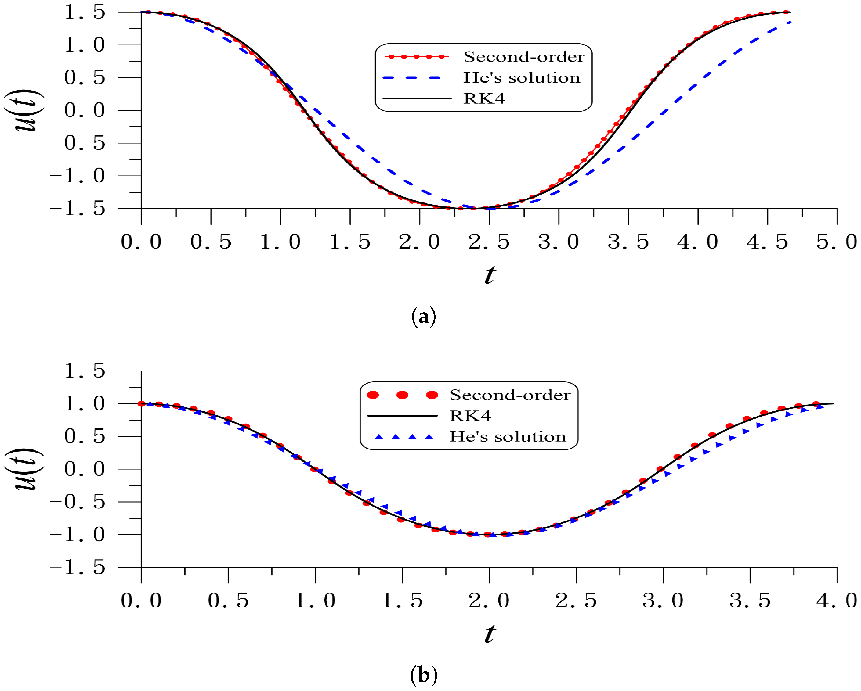
We show this in Figure 1a by the blue-dashed line of the first-order periodic solution (5) obtained for the Micken’s oscillator in Equation (32) with $A=1.5$; also refer to Figure 1d in [15], where $\omega$ is obtained from Equation (34). We can observe that the first-order periodic solution, which is named He’s solution in the figure, is not accurate.

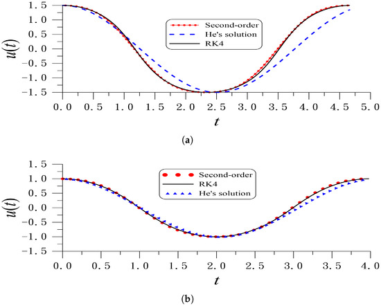
Figure 1. For (a) Mickens’ oscillator and (b) the vibration of a tapered beam, we compare RK4 solution and the periodic solution obtained by the second-order solution from the LRGM and He’s first-order solution—shortened as He’s solution.

To improve the accuracy of the periodic solution, we consider a more accurate second-order analytic solution, which is given by

$$u\left(t\right)=(A-B)cos\omega t+Bcos3\omega t,$$

(89)

where $\omega$ and B are both unknown constants. If we directly insert Equation (89) into Equation (4), the residual function would be very complicated, which hinders the development of an effective Galerkin method. Before that, we will linearize Equation (4) with respect to the first-order solution (5). Then, we can derive a linearized residual, and then the Galerkin method is applied. Below, we employ the Micken’s oscillator and a tapered beam’s oscillator to demonstrate the linearized residual Galerkin method (LRGM).

(A) Micken’s oscillator. If we inserted Equation (89) into Equation (32), it would be quite complicated to solve $\omega$ and B by some nonlinear algebraic equations. At the very beginning, we linearize Equation (32) to

$$\ddot{u}\left(t\right)+u\left(t\right)+q_0{u}_0\left(t\right){\dot{u}}_0\left(t\right)\dot{u}\left(t\right)=(q_0-1)u_0\left(t\right){\dot{u}}_0^2\left(t\right),$$

(90)

where $q_0$ is a weight factor. Inserting $u_0\left(t\right)=Acos\omega t$ into Equation (90) leads to

$$\ddot{u}\left(t\right)+u\left(t\right)-a_0(1-cos2\omega t)\dot{u}\left(t\right)=b_0(cos\omega t-cos3\omega t),$$

(91)

where

$$a_0={\displaystyle \frac{q_0{A}^2{\omega }^2}{4}},b_0={\displaystyle \frac{(q_0-1)A^3{\omega }^2}{4}}.$$

(92)

Equation (91) is a second-order linear ordinary differential equation for $u\left(t\right)$. Inserting Equation (89) into Equation (91), the linearized residual is

$$\begin{array}{c}{R}_L\left(t\right)={\omega }^2(B-A)cos\omega t-9{\omega }^{2}Bcos3\omega t+(A-B)cos\omega t+Bcos3\omega t\hfill \\ +a_0(A+2B)cos\omega t-a_0(A-B)cos3\omega t-3B{a}_{0}cos3\omega t-b_{0}cos3\omega t+b_{0}cos3\omega t.\hfill \end{array}$$

(93)

Basing on the Galerkin method, we impose two weighted residual equations to determine $\omega$ and B:

$${\int }_0^T{R}_L\left(t\right)cos\omega tdt=0,{\int }_0^T{R}_L\left(t\right)cos3\omega tdt=0,$$

(94)

which through some manipulations generate

$$B({\omega }^2-1+2a_0)=b_0+A({\omega }^2-1-a_0),B(9{\omega }^2-1-a_0)=b_0-a_{0}A.$$

(95)

Hence, by means of Equations (92) and (95), one can derive

$$\omega =\sqrt{{\displaystyle \frac{-d_0-\sqrt{d_0^2+64c_0}}{2c_0}}},B={\displaystyle \frac{A^3{\omega }^2}{4+q_0{A}^2{\omega }^2-36{\omega }^2}},$$

(96)

where

$$c_0=4q_0{A}^2-3q_0{A}^4+32A^2-144,d_0=160-4q_0{A}^2.$$

(97)

Inserting Equation (96) into Equation (89) yields the second-order periodic solution obtained by the linearized residual Galerkin method (LRGM). Take $q_0=0.99919$; the red line in Figure 1a is compared to the thick black line of the so-called “exact solution”, which is obtained by applying the fourth-order Runge–Kutta method to integrate Equation (32) with $A=1.5$. The exact frequency given by Equation (36) is 1.34868997, which is very close to the value of 1.34868945 obtained by Equation (96). The improvement of the accuracy of the frequency and the second-order periodic solution obtained by the LRGM is significant. To obtain an approximate “exact solution”, we have applied the RK4 to integrate the nonlinear ODE with the given initial conditions. The “exact solution” is remarked as the RK4 solution in the figure.

(B) Tapered beam’s oscillator. Next, we apply the LRGM to the tapered beam’s oscillator in Equation (37), which is linearized with respect to $u_0=Acos\omega t$:

$$\ddot{u}+u+q_{0}a{u}_0{\ddot{u}}_{0}u+q_{0}a{u}_0{\dot{u}}_0\dot{u}+q_{0}b{u}_0^{2}u=(q_0-1)[a{u}_0^2{\ddot{u}}_0+a{u}_0{\dot{u}}_0^2+b{u}_0^3].$$

(98)

Inserting Equation (89) into Equation (98) results in a linearized residual:

$$\begin{array}{c}{R}_L\left(t\right)={\omega }^2(B-A)cos\omega t-9{\omega }^{2}cos3\omega t+(A-B+e_3-e_1)cos\omega t+(B+e_3-e_2)cos3\omega t\hfill \\ +e_{3}cos2\omega t[(A-B)cos\omega t+Bcos3\omega t]+e_4\omega sin2\omega t[(A-B)sin\omega t+3Bsin3\omega t],\hfill \end{array}$$

(99)

where

$$\begin{array}{c}{e}_1={\displaystyle \frac{3(q_0-1)b{A}^3}{4}}-{\displaystyle \frac{(q_0-1)a{A}^3{\omega }^2}{2}},e_2={\displaystyle \frac{(q_0-1)b{A}^3}{4}}-{\displaystyle \frac{(q_0-1)a{A}^3{\omega }^2}{2}},\hfill \\ e_3={\displaystyle \frac{q_{0}b{A}^2}{2}}-{\displaystyle \frac{q_{0}a{A}^2{\omega }^2}{2}},e_4={\displaystyle \frac{q_{0}a{A}^2\omega }{2}}.\hfill \end{array}$$

(100)

By using the LRGM, we can derive

$$\omega =\sqrt{{\displaystyle \frac{-b_0-\sqrt{b_0^2-4a_0{c}_0}}{2a_0}}},B={\displaystyle \frac{A_0{\omega }^2-B_0}{(2q_{0}a{A}^2+4){\omega }^2-4}},$$

(101)

where

$$\begin{array}{c}{A}_0=4A+2q_{0}a{A}^2-2(q_0-1)a{A}^3,B_0=4A+2q_{0}b{A}^2-(2q_0-3)b{A}^3,\hfill \end{array}$$

$$\begin{array}{c}{C}_0=2q_{0}a{A}^2+2a{A}^3,D_0=2q_{0}b{A}^2+b{A}^3,\hfill \\ a_0=A_0(3q_{0}a{A}^2-36)-C_0(2q_{0}a{A}^2+4),c_0=-B_0(4-q_{0}b{A}^2)-4D_0,\hfill \end{array}$$

(102)

$$\begin{array}{c}{b}_0=A_0(4-q_{0}b{A}^2)-B_0(3q_{0}a{A}^2-36)+4C_0+D_0(2q_{0}a{A}^2+4).\hfill \end{array}$$

(103)

With $A=1$, $a=2$, and $b=5$, Figure 1b shows the first-order solution (5) with $\omega =1.541104$ computed from Equation (38), which is named He’s solution, and the RK4 solution, and the second-order periodic solution obtained by the LRGM are compared. With $q_0=-2.83$, we obtain $\omega =1.58033$, which is close to the exact one with $\omega =1.58031$; moreover, the accuracy of the second-order periodic solution obtained by the LRGM is improved compared to the first-order one by about one order.

8. The Applications of Theorem 3 and LRGM

In order to demonstrate the applications of Theorem 3 and more results obtained from the LRGM, some examples are given below. Equation (81) used for seeking the frequency is a simply linearly perturbed equation of the original frequency equation, which can help us to quickly obtain a very precise value of the frequency for the nonlinear oscillator. We will also examine a hybrid method obtained by combining Equation (81) and the LRGM.

Similarly, the value of $\alpha$ used in the hybrid method is determined by the following numerical method. We determine the value of $\alpha$ by subjecting it to Equation (24). In the minimization problem with a single unknown value $\alpha$, the interval reduction method (IRM) is adopted to find the optimal value of $\alpha$.

8.1. A Nonlinear Oscillator with Irrational Restoring Force

We consider an irrational restoring force in the nonlinear oscillator [38]:

$$\ddot{u}\left(t\right)+u\left(t\right)-{\displaystyle \frac{\lambda u\left(t\right)}{\sqrt{1+u^2\left(t\right)}}}=0,u\left(0\right)=A,\dot{u}\left(0\right)=0,$$

(104)

where $0<\lambda \le 1$ is a constant.

Inserting Equation (5) into the following equation yields

$${(\ddot{u}+u)}^2(1+u^2)-{\lambda }^2{u}^2=0,$$

(105)

Zhao [38] derived the residual as

$$R\left(t\right)=A^2(1+A^2{cos}^2\omega t)(1-{\omega }^2){cos}^2\omega t-A^2{\lambda }^2{cos}^2\omega t.$$

(106)

By the Galerkin method, it follows that

$$\tilde{R}\left({\omega }^2\right)={\displaystyle \frac{1}{15\pi }}[20A^2(1-{\omega }^2-{\lambda }^2)+16A^4(1-{\omega }^2)].$$

(107)

Taking ${\omega }_1^2=1$ and ${\omega }_2^2=2$, He’s frequency–amplitude formula reads as

$${\omega }^2={\displaystyle \frac{{\omega }_1^2{\tilde{R}}_2-{\omega }_2^2{\tilde{R}}_1}{{\tilde{R}}_2-{\tilde{R}}_1}}=1-{\displaystyle \frac{5{\lambda }^2}{5+4A^2}}.$$

(108)

As an application of Equation (81) in Theorem 3, we take

$$x={\omega }^2,x_1={\omega }_1^2=1,F\left({\omega }^2\right)={\omega }^2-1+{\displaystyle \frac{5{\lambda }^2}{5+4A^2}}.$$

(109)

Inserting them into Equation (81), we propose the following new frequency–amplitude formula:

$${\omega }^2=1-{\displaystyle \frac{5{\lambda }^2}{5+4A^2+5\alpha {\lambda }^2}}.$$

(110)

If $\alpha =0$, Equation (110) recovers to Equation (108). The optimal value of $\alpha$ is obtained by satisfying the periodicity condition $u\left(T\right)-A=0$.

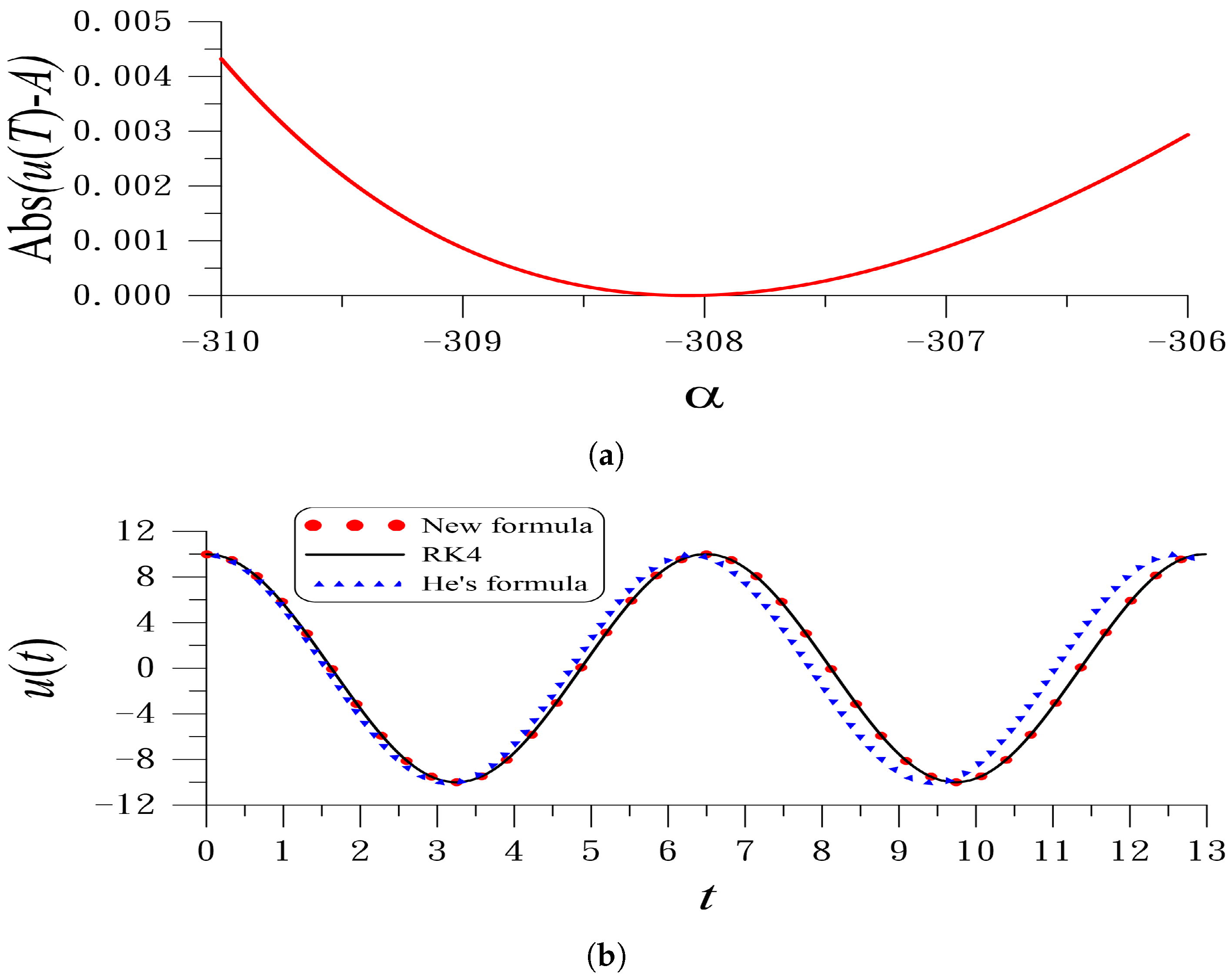
Under the following values of $A=10$ and $\lambda =0.5$, Figure 2a shows the error of Abs($u\left(T\right)-A$) plotted with respect to $\alpha \in [-310,-306]$. There exists a minimal point of the curve. When $\alpha =0$, Abs($u\left(T\right)-A$) = 0.184, which shows that the accuracy of $\omega =0.9984556$ obtained from Equation (108) is not accurate. On the other hand, when $\alpha =-308.05$, we obtain $\omega =0.96814466$, and the error of Abs($u\left(T\right)-A$) is drastically reduced to Abs($u\left(T\right)-A)=3.84\times {10}^{-7}$. In Figure 2b, the exact solution of Equation (104) within two periods is compared to the periodic solution $u\left(t\right)=Acos\omega t$, with $\omega$ obtained from Equations (108) and (110). It is apparent that the periodic solution obtained from Equation (110) is more accurate than that obtained from Equation (108). The maximal error (ME) = 3.38 for Equation (108) is significantly reduced to ME = $4.29\times {10}^{-2}$ for Equation (110).

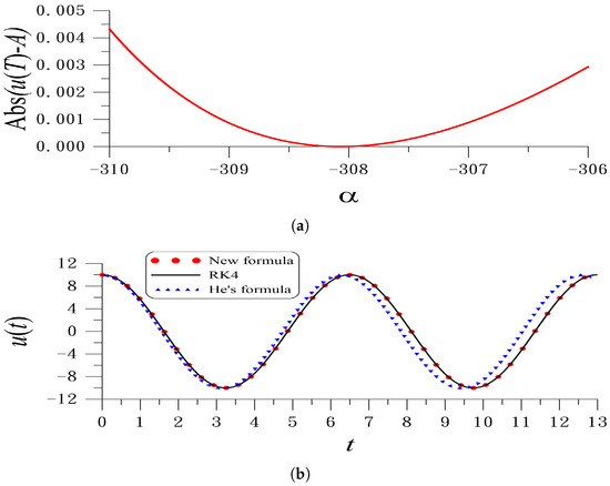
Figure 2. For the irrational restoring force oscillator in Equation (104), (a) shows the error of the periodicity condition with respect to $\alpha$, and (b) compares the RK4 solution and the first-order periodic solutions obtained by He’s formula and the new formula.

8.2. A Nonconservative Nonlinear Oscillator

To further demonstrate the application of Theorem 3, we consider a damped nonlinear oscillator [39]:

$$\ddot{u}\left(t\right)+{\displaystyle \frac{ku\left(t\right)}{1+c{\dot{u}}^2\left(t\right)}}+bu\left(t\right)=0,u\left(0\right)=A,\dot{u}\left(0\right)=0,$$

(111)

where k, c, and b are some constants. As derived in [39], the corresponding residual is

$$R\left(t\right)=(b+k-{\omega }^2)Acos\omega t+{\omega }^{2}c{A}^3(b-{\omega }^2){sin}^2\omega tcos\omega t.$$

(112)

By using the Galerkin method, we come to a weighted residual equation:

$$\tilde{R}\left({\omega }^2\right)=c{A}^2{\omega }^4+(4-bc{A}^2){\omega }^2-4(b+k)=0.$$

(113)

The following formula was derived in [39]:

$$\omega =\sqrt{{\displaystyle \frac{bc{A}^2-4+\sqrt{{(bc{A}^2-4)}^2+16c{A}^2(b+k)}}{2c{A}^2}}},$$

(114)

which is the same as that obtained by the homotopy perturbation method [40].

However, we found that the accuracy of Equation (114) is not so good. Let

$$F\left(x\right)=\tilde{R}\left({\omega }^2\right)=c{A}^2{\omega }^4+(4-bc{A}^2){\omega }^2-4(b+k),x={\omega }^2.$$

(115)

By means of Equation (81) in Theorem 3 with $x_1={\omega }_1^2=1$, we can modify Equation (113) to

$$c{A}^2{\omega }^4+(4-bc{A}^2){\omega }^2-4(b+k)+\alpha ({\omega }^2-1)[c(1-b)A^2-4(b+k)+4]=0,$$

(116)

which is arranged to

$$c{A}^2{\omega }^4+[4-bc{A}^2+\alpha (c(1-b)A^2-4b-4k+4)]{\omega }^2-[4b+4k+\alpha (c(1-b)A^2-4b-4k+4)]=0.$$

(117)

The frequency–amplitude formula is modified to

$$\omega =\sqrt{{\displaystyle \frac{e_1+\sqrt{e_1^2+16c{A}^2{e}_2}}{2c{A}^2}}},$$

(118)

where

$$e_1=bc{A}^2-4-\alpha (c(1-b)A^2-4b-4k+4),e_2=4b+4k+\alpha (c(1-b)A^2-4b-4k+4).$$

(119)

If $\alpha =0$, Equation (118) recovers to Equation (114). The optimal value of $\alpha$ is obtained by satisfying the periodicity condition $u\left(T\right)-A=0$.

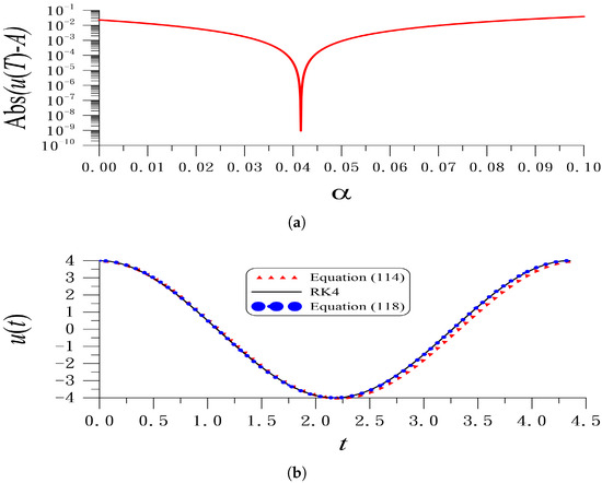
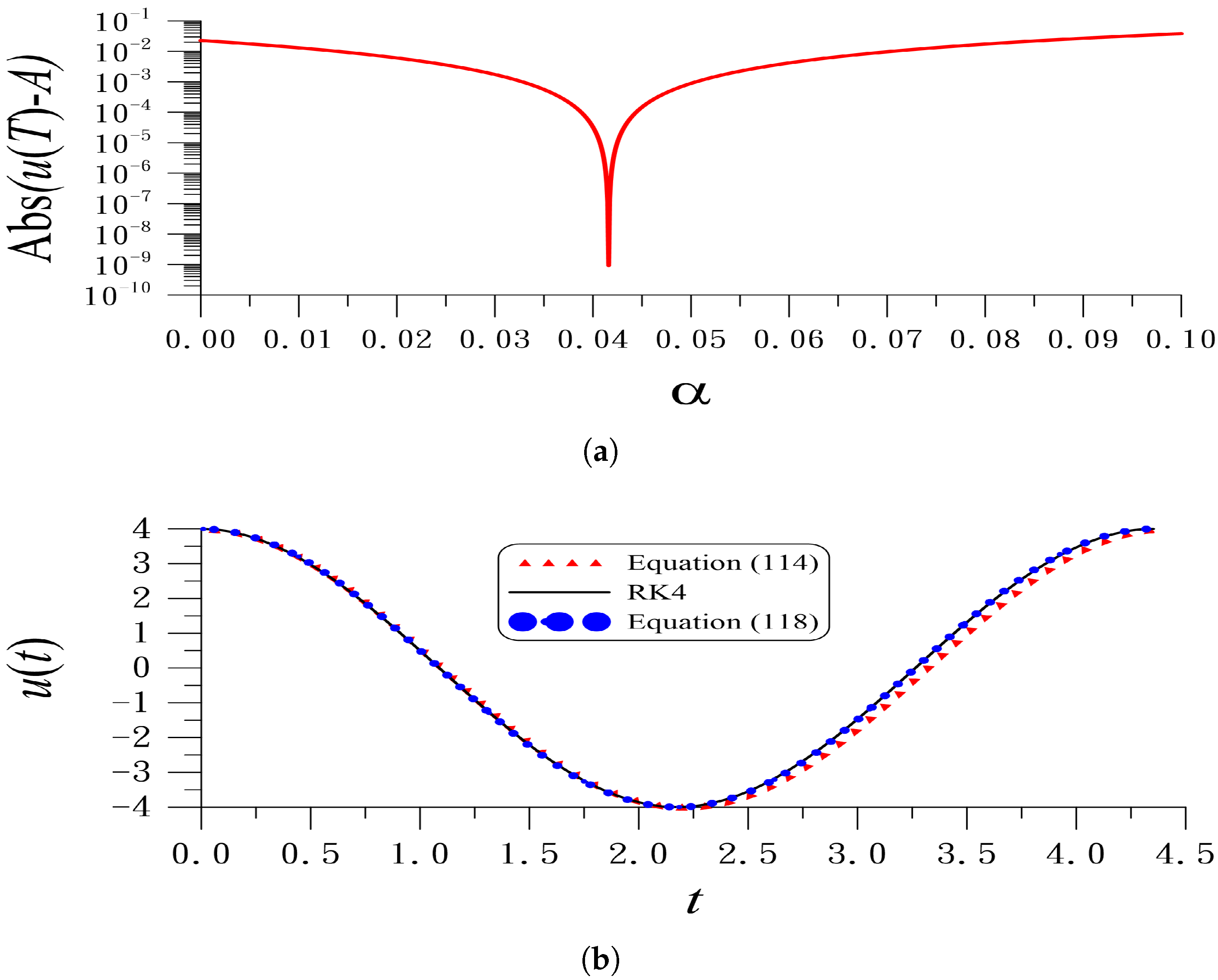
Under the following values of $A=4$, $k=0.5$, $b=2$, and $c=3$, Figure 3a shows the error of Abs($u\left(T\right)-A$) plotted with respect to $\alpha \in [0,0.1]$. When $\alpha =0$, Abs($u\left(T\right)-A$) = 0.02278, which reveals that the accuracy of $\omega$ obtained from Equation (118) is not very good. On the other hand, when $\alpha =0.0416$, the error of Abs($u\left(T\right)-A$) is significantly reduced to Abs($u\left(T\right)-A)=9.2284\times {10}^{-10}$. In Figure 3b, the RK4 solution of Equation (111) is compared to the periodic solution $u\left(t\right)=Acos\omega t$, with $\omega$ obtained from Equations (114) and (118). It is apparent that the periodic solution obtained from Equation (118) is more accurate than that obtained from Equation (114).

Figure 3. For the damped oscillator in Equation (111), (a) shows the error of periodicity condition with respect to $\alpha$, and (b) compares the RK4 solution and the first-order periodic solutions obtained by Equations (114) and (118).

In order to apply the LRGM to find the second-order periodic solution of Equation (111), we linearize it with respect to $u_0=Acos\omega t$:

$$\ddot{u}+(b+k)u+q_{0}c{\dot{u}}_0{\ddot{u}}_0\dot{u}+q_{0}bc{\dot{u}}_0^{2}u=(q_0-1)(c{\dot{u}}_0^2{\ddot{u}}_0+bc{\dot{u}}_0^2{u}_0),$$

(120)

which, after inserting Equation (89), results in a linearized residual:

$$\begin{array}{c}{R}_L\left(t\right)={\omega }^2(B-A)cos\omega t-9{\omega }^{2}Bcos3\omega t+d_4(A-B)cos\omega t+d_{4}Bcos3\omega t\hfill \\ -{\displaystyle \frac{d_1\omega (A+B)}{2}}cos\omega t-{\displaystyle \frac{d_1\omega (B-A)}{2}}cos3\omega t+{\displaystyle \frac{3d_1\omega B}{2}}cos5\omega t\hfill \\ -{\displaystyle \frac{d_{3}A}{2}}cos\omega t+{\displaystyle \frac{d_3(B-A)}{2}}cos3\omega t-d_{2}cos\omega t+d_{2}cos3\omega t,\hfill \end{array}$$

(121)

where

$$d_1={\displaystyle \frac{q_{0}c{A}^2{\omega }^3}{2}},d_2={\displaystyle \frac{(q_0-1)c{A}^3{\omega }^2}{4}}(b-{\omega }^2),d_3={\displaystyle \frac{q_{0}bc{A}^2{\omega }^2}{2}},d_4=b+k+e_3.$$

(122)

It can be seen that $R_L\left(t\right)$ is a nonlinear function of the frequency up to the fourth order. For simplicity, we employ a hybrid method by using Equation (118) to compute $\omega$ and then use the LRGM to determine B.

By using the LRGM and under the following Galerkin condition, we have

$${\int }_0^T{R}_L\left(t\right)cos3\omega tdt=0,$$

(123)

and we can derive

$$B={\displaystyle \frac{d_1\omega A-d_{3}A+2d_2}{18{\omega }^2-2d_4+d_1\omega -d_3}}.$$

(124)

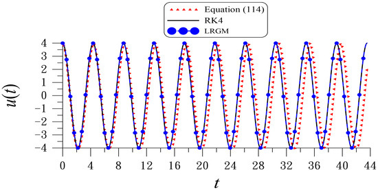
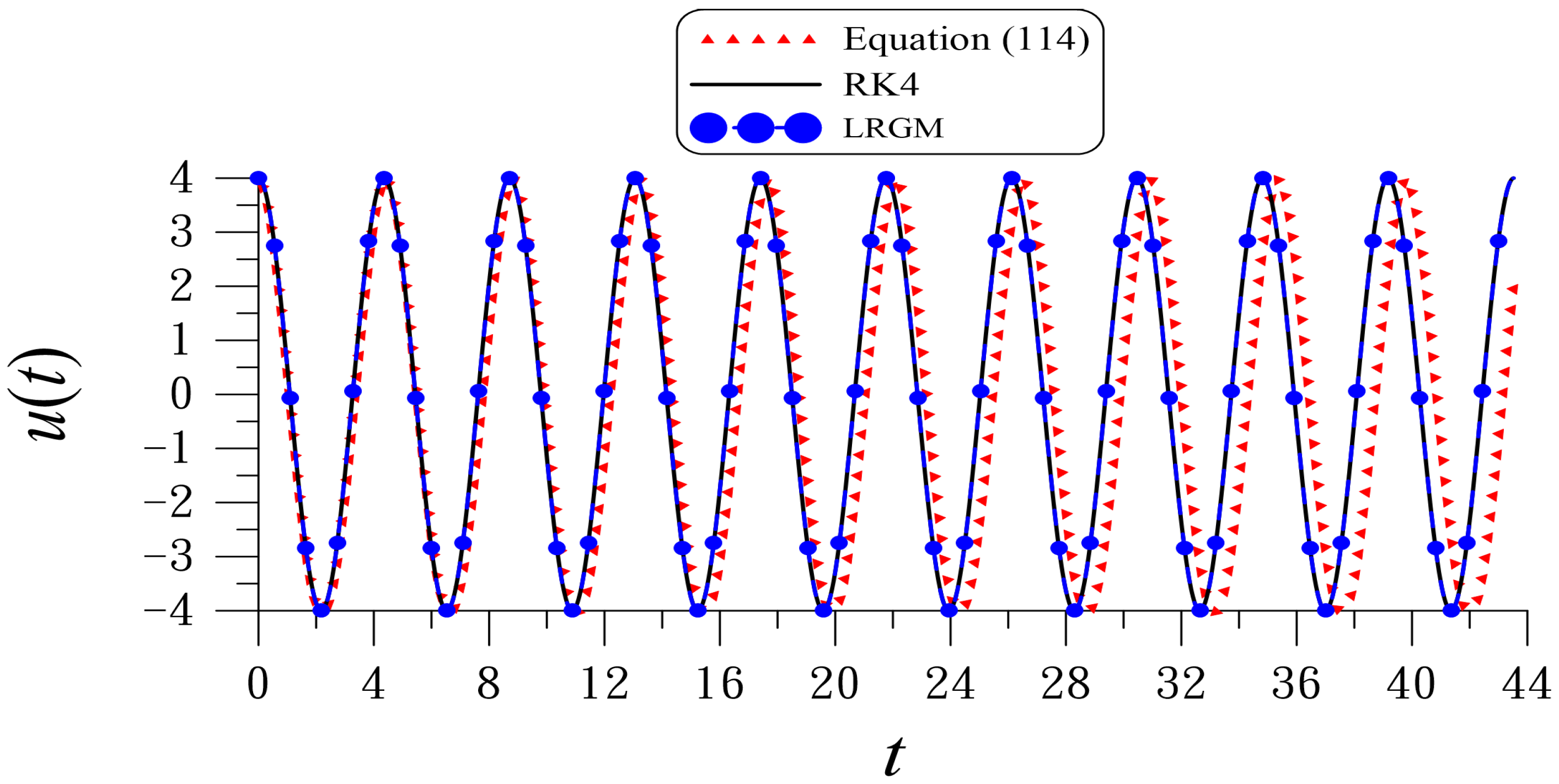
Inserting $\omega$ and B into Equation (89), we can derive the second-order periodic solution of Equation (111). Considering the following values of $A=4$, $k=0.5$, $b=2$, $c=3$, and $q_0=0.0408$, Figure 4 shows the periodic solution up to ten periods compared to that computed by Equation (114). It is apparent that the periodic solution obtained from the second-order periodic solution obtained from the LRGM is much more accurate than that obtained from Equation (114). Even up to the tenth period, the second-order periodic solution obtained from the LRGM is almost coincident to the RK4 solution with the maximal error (ME) = $9.63\times {10}^{-3}$, but the solution $Acos\omega t$ with $\omega$ obtained from Equation (114) is gradually digressed to the RK4 solution with ME = 3.66.

Figure 4. For the damped oscillator in Equation (111), compare the RK4 solution and the periodic solutions obtained by Equation (114) and the second-order periodic solution obtained from a hybrid method of the LRGM.

8.3. A Cubic-Quintic Duffing Nonlinear Oscillator

We consider a cubic-quintic Duffing nonlinear oscillator [41]:

$$\ddot{u}\left(t\right)+u\left(t\right)+{\epsilon }_0{u}^3\left(t\right)+c{u}^5\left(t\right)=0,u\left(0\right)=A,\dot{u}\left(0\right)=0,$$

(125)

where ${\epsilon }_0$ and c are some constants. When $c=0$, it reduces to the Duffing oscillator in Equation (25).

The Hamiltonian-based frequency formulation [42] is a modification of He’s frequency formulation [31]. Because the Hamiltonian-based frequency–amplitude formulation takes account of the energy of the nonlinear vibration system to establish the corresponding Hamilton principle, its approximate solution is valid for the whole solution domain without the limitations such as those in the traditional perturbation method.

Let

$$P\left(u\right)={\displaystyle \frac{1}{2}}{u}^2+{\displaystyle \frac{{\epsilon }_0}{4}}{u}^4+{\displaystyle \frac{c}{6}}{u}^6$$

(126)

be the potential function of the restoring force.

According to [42], Ma [41] derived a simple frequency–amplitude formula:

$${\omega }^2={\displaystyle \frac{4[P\left(A\right)-P(A/\sqrt{2})]}{A^2}}.$$

(127)

Inserting Equation (126) into Equation (127) yields Ma’s frequency–amplitude formula:

$${\omega }^2=1+{\displaystyle \frac{3}{4}}{\epsilon }_0{A}^2+{\displaystyle \frac{7}{12}}c{A}^4.$$

(128)

Let

$$\tilde{R}\left({\omega }^2\right)={\omega }^2-1-{\displaystyle \frac{3}{4}}{\epsilon }_0{A}^2-{\displaystyle \frac{7}{12}}c{A}^4.$$

(129)

According to Equation (81) in Theorem 3, we can generate a new frequency equation:

$${\omega }^2-1-{\displaystyle \frac{3}{4}}{\epsilon }_0{A}^2-{\displaystyle \frac{7}{12}}c{A}^4-\alpha ({\omega }^2-1)\left[{\displaystyle \frac{3}{4}}{\epsilon }_0{A}^2+{\displaystyle \frac{7}{12}}c{A}^4\right]=0.$$

(130)

It follows a new frequency–amplitude formula:

$${\omega }^2=1+{\displaystyle \frac{9{\epsilon }_0{A}^2+7c{A}^4}{12-\alpha (9{\epsilon }_0{A}^2+7c{A}^4)}}.$$

(131)

If $\alpha =0$, Equation (131) recovers to Equation (130). The optimal value of $\alpha$ is obtained to satisfy the periodicity condition $u\left(T\right)-A=0$.

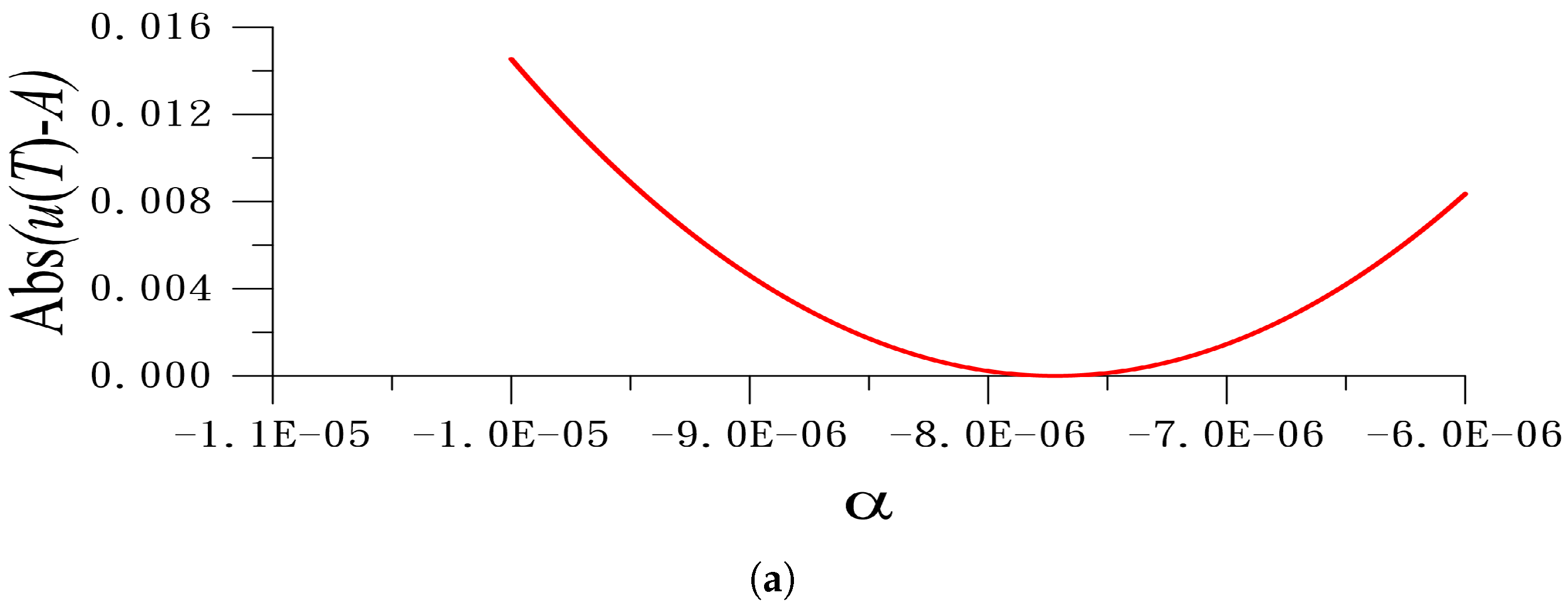
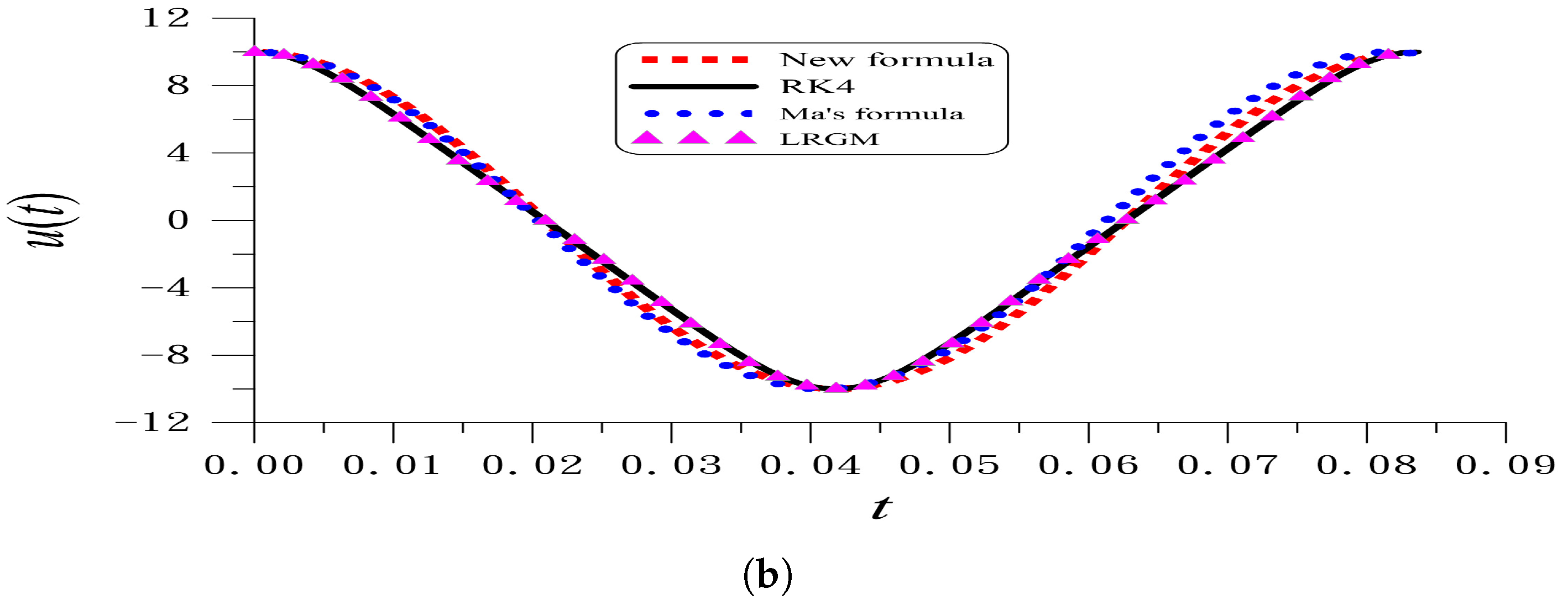
Under the following values of $A=10$ and ${\epsilon }_0=c=1$, Figure 5a shows the error of Abs($u\left(T\right)-A$) plotted with respect to $\alpha \in [-{10}^{-5},-6\times {10}^{-6}]$. There exists a minimal point of the curve. When $\alpha =0$, Abs($u\left(T\right)-A$) = 0.169, which reveals that the value of $\omega =76.872188$ obtained from Equation (130) is not accurate. When $\alpha =-7.72\times {10}^{-6}$, we obtain $\omega =75.177101$, and the error of Abs($u\left(T\right)-A$) is drastically reduced to Abs($u\left(T\right)-A)=5.63\times {10}^{-9}$. Figure 5b shows the RK4 solution of Equation (125) compared to the periodic solution $u\left(t\right)=Acos\omega t$, with $\omega$ obtained from Equations (130) and (131). The accuracy of the first-order periodic solution obtained from Equation (131) is improved compared to that obtained from Equation (130).

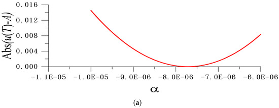
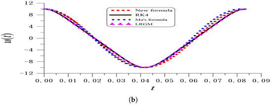
Figure 5. For the cubic-quintic Duffing nonlinear oscillator in Equation (125), (a) shows the error of periodicity condition with respect to $\alpha$, and (b) compares the RK4 solution and the periodic solutions obtained by Ma’s formula, the new formula, and the second-order periodic solution obtained from a hybrid method of the LRGM.

To find the second-order periodic solution from the LRGM, we linearize Equation (125) to

$$\ddot{u}\left(t\right)+u\left(t\right)+q_0{\epsilon }_0{u}_0^2\left(t\right)u\left(t\right)+q_{0}c{u}_0^4\left(t\right)u\left(t\right)=(q_0-1)[{\epsilon }_0{u}_0^3\left(t\right)+c{u}_0^5\left(t\right)].$$

(132)

We can derive $R_L\left(t\right)$ after inserting Equation (89) into Equation (132). Using the LRGM and subjecting to

$${\int }_0^T{R}_L\left(t\right)cos3\omega tdt=0,$$

(133)

we can derive

$$B={\displaystyle \frac{4{\epsilon }_0{A}^3+5c{A}^5}{16+4q_0{\epsilon }_0{A}^2+q_{0}c{A}^4-144{\omega }^2}},$$

(134)

where $\omega$ is computed by Equation (131).

Inserting $\omega$ and B into Equation (89), we can derive the second-order periodic solution of Equation (125). This is a hybrid method to solve Equation (125).

Given $A=10$, ${\epsilon }_0=c=1$, and $q_0=150$, Figure 5b shows the second-order periodic solution compared to the RK4 solution, which is almost coincident with ME = 0.134; it is much smaller than the ME = 1.95 value computed by Ma’s formula (128).

8.4. The Helmholtz–Duffing Nonlinear Oscillator

We consider the Helmholtz–Duffing nonlinear oscillator [43,44,45,46]:

$$\ddot{u}\left(t\right)+a_{1}u\left(t\right)-a_2{u}^2\left(t\right)+a_3{u}^3\left(t\right)=0,u\left(0\right)=A,\dot{u}\left(0\right)=0,$$

(135)

where $a_1$, $a_2$, and $a_3$ are some constants. When $a_2=0$, it reduces to the Duffing oscillator in Equation (25).

Because Equation (135) is not a symmetric oscillator, we consider the following solution:

$$u\left(t\right)=(A+B)cos\omega t-B.$$

(136)

We can derive $R_L\left(t\right)$ after inserting Equation (136) into Equation (135), and using the Galerking method, we can derive a frequency equation:

$$\tilde{R}\left({\omega }^2\right)={\omega }^2-a_1-{\displaystyle \frac{3a_3}{4}}{(A+B)}^2-2a_{2}B=0,$$

(137)

where B can be obtained by applying the Cardan’s formula to the following cubic equation:

$$B^3-{\displaystyle \frac{3a_2}{a_3}}{B}^2-\left[{\displaystyle \frac{2a_1}{a_3}}+3A^2+{\displaystyle \frac{2a_2}{a_3}}A\right]B-{\displaystyle \frac{a_2}{a_3}}{A}^2=0.$$

(138)

Upon taking $x={\omega }^2$, $F\left(x\right)=\tilde{R}\left({\omega }^2\right)$ and $x_1={\omega }_1^2=0$, by means of Equation (82) in Theorem 3, we can derive a new frequency equation:

$${\omega }^2-a_1-{\displaystyle \frac{3a_3}{4}}{(A+B)}^2-2a_{2}B-\alpha {\omega }^2\left[a_1+{\displaystyle \frac{3a_3}{4}}{(A+B)}^2+2a_{2}B\right]=0,$$

(139)

which leads to a new frequency formula:

$${\omega }^2={\displaystyle \frac{a_1+\frac{3a_3}{4}{(A+B)}^2+2a_{2}B}{1-\alpha [a_1+\frac{3a_3}{4}{(A+B)}^2+2a_{2}B]}}.$$

(140)

According to [43], El-Dib’s formulas for ${\omega }^2$ and B are

$${\omega }^2=a_1+{\displaystyle \frac{3a_3}{4}}{A}^2,B={\displaystyle \frac{1}{4{\omega }^2}}{a}_2{A}^2.$$

(141)

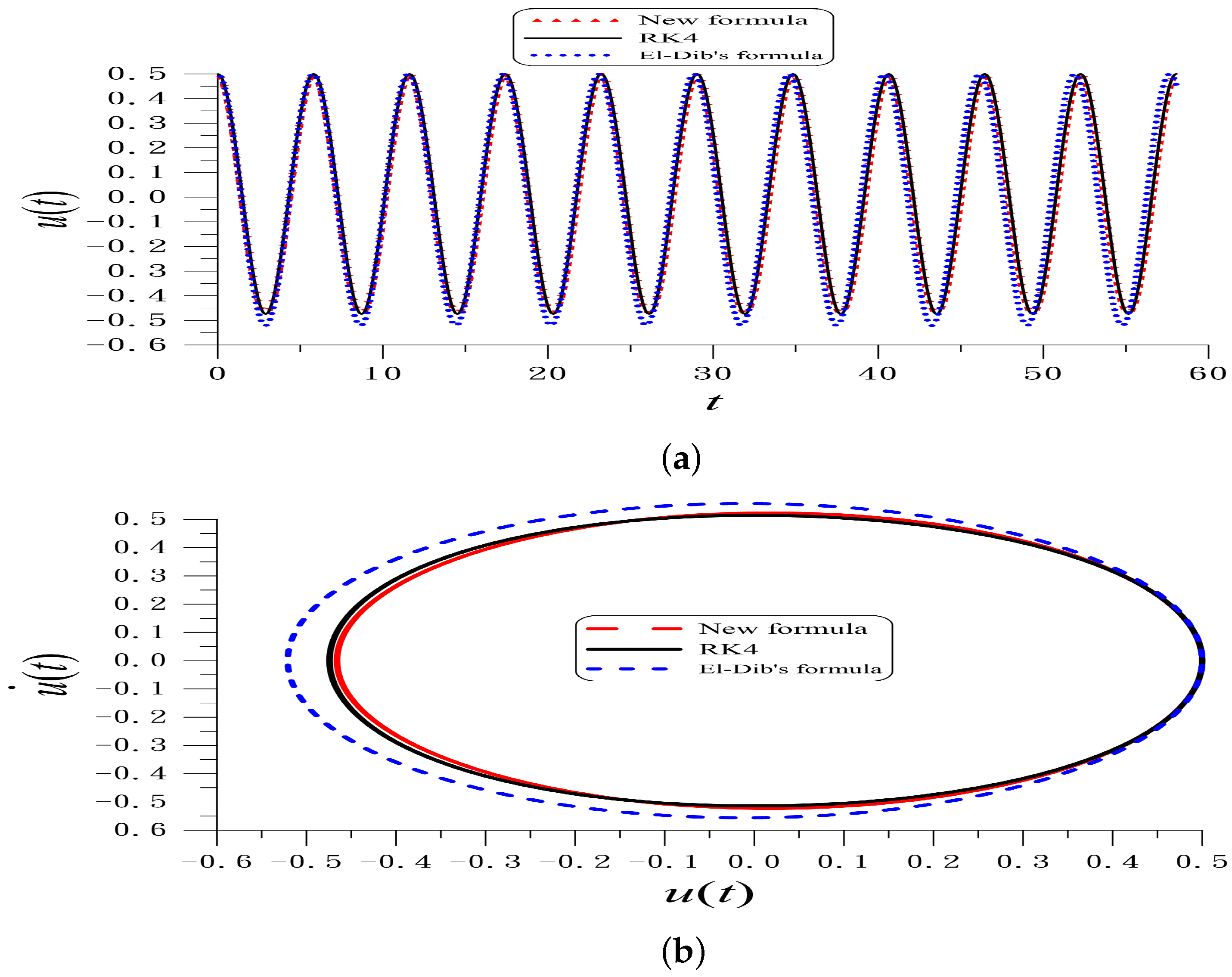
Inserting $\omega$ and B into Equation (136), we can derive the first-order periodic solution of Equation (135). Given $A=0.5$, $a_1=1$, $a_2=0.5$, and $a_3=1$, $\omega =1.08972474$ and $B=0.01052632$ are obtained from Equation (141); $\omega =1.08232452$ and $B=-0.01700967$ are obtained from Equation (140) with $\alpha =0.00239$ and Equation (138). Figure 6a shows the first-order periodic solutions compared to the RK4 solution within ten periods. The first-order periodic solution is obtained from Equations (136), (138) and (140) is almost coincident to the RK4 solution with ME = $8.39\times {10}^{-3}$; it is much smaller than the ME = 0.2313 value obtained by El-Dib’s formula (141). As shown in Figure 6b, the phase portrait obtained from El-Dib’s Formula (141) overestimates the amplitude.

Figure 6. For the Helmholtz–Duffing nonlinear oscillator within ten periods comparing (a) time histories and (b) phase portraits of RK4 solution and the periodic solutions obtained by El-Dib’s formula and new formula.

9. Higher-Order Periodic Solutions of Duffing Oscillator

Notice that when $c=0$, Equation (131) is recovered to Equation (29) for the Duffing oscillator; B in Equation (134) is reduced to

$$B={\displaystyle \frac{{\epsilon }_0{A}^3}{4+q_0{\epsilon }_0{A}^2-36{\omega }^2}}.$$

(142)

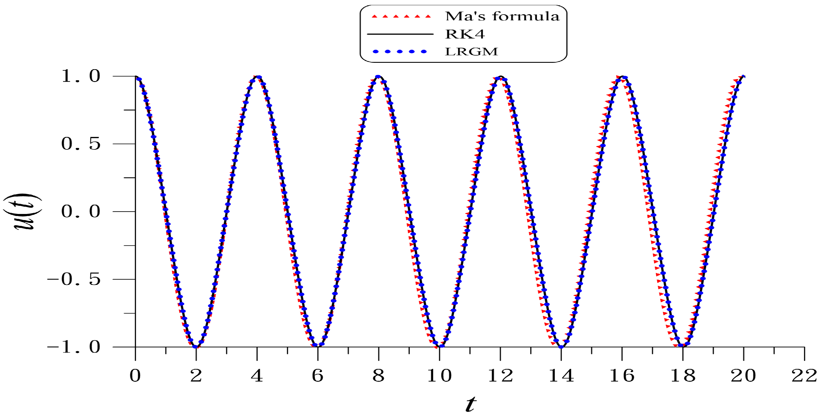
Inserting $\omega$ and B into Equation (89), we can derive the second-order periodic solution of Equation (25) by using the hybrid method. Given $A=1$, ${\epsilon }_0=2$, $\alpha =-0.017284$, and $q_0=81.35$, Figure 7 shows the second-order periodic solution within five periods compared to the RK4 solution, which is almost coincident with ME = $8.57\times {10}^{-4}$; it is much smaller than the ME = 0.238 value computed by Ma’s formula (128). The exact frequency is $\omega =1.5691058$; $\omega =1.5811388$ by Ma’s formula (128); and $\omega =1.569106$ by the new Formula (29). It is apparent that the accuracy of frequency is raised from two orders to seven orders by the new formula.

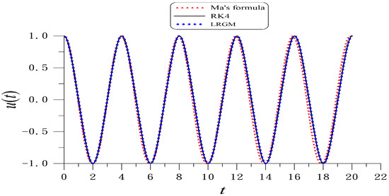
Figure 7. For the Duffing nonlinear oscillator within five periods comparing RK4 solution and the periodic solution obtained by Ma’s formula and the second-order periodic solution obtained from a hybrid method of the LRGM.

Basically, when we extend the second-order periodic solution to the third-order periodic solution by using the LRGM, we can extend Equation (89) to

$$u\left(t\right)=(A-B-C)cos\omega t+Bcos3\omega t+Ccos5\omega t.$$

(143)

The three constants B, C, and $\omega$ are determined by using three Galerkin conditions:

$${\int }_0^T{R}_L\left(t\right)cos\omega tdt=0,{\int }_0^T{R}_L\left(t\right)cos3\omega tdt=0,{\int }_0^T{R}_L\left(t\right)cos5\omega tdt=0,$$

(144)

which, after inserting the linearized residual function $R_L\left(t\right)$, results in three algebraic equations to determine B, C, and $\omega$.

We take the Duffing oscillator as an example to seek the third-order periodic solution. The first step is to linearize the Duffing Equation (25) with respect to $u_0=Acos\omega t$:

$$\ddot{u}\left(t\right)+u\left(t\right)+{\displaystyle \frac{q_0{\epsilon }_0{A}^2}{2}}(1+cos2\omega t)u\left(t\right)={\displaystyle \frac{(q_0-1){\epsilon }_0{A}^3}{4}}(3cos\omega t+cos3\omega t).$$

(145)

After inserting Equation (143), $R_L\left(t\right)$ can be derived as follows:

$$\begin{array}{c}{R}_L\left(t\right)=(B+C-A){\omega }^{2}cos\omega t-9B{\omega }^{2}cos3\omega t-25C{\omega }^{2}cos5\omega t\hfill \\ +(A-B-C)cos\omega t+Bcos3\omega t+Ccos5\omega t\hfill \\ +{\displaystyle \frac{q_0{\epsilon }_0{A}^2}{2}}[(A-B-C)cos\omega t+Bcos3\omega t+Ccos5\omega t]-{\displaystyle \frac{(q_0-1){\epsilon }_0{A}^3}{4}}(3cos\omega t+cos3\omega t)\hfill \\ +{\displaystyle \frac{q_0{\epsilon }_0{A}^2}{4}}[(A-B-C)cos\omega t+(A-B-C)cos3\omega t\hfill \\ +Bcos\omega t+Bcos5\omega t+Ccos3\omega t+Ccos7\omega t].\hfill \end{array}$$

(146)

The second step is inserting $R_L\left(t\right)$ into Equation (144), which results in

$$\begin{array}{c}(B+C-A)({\omega }^2-1)-{\displaystyle \frac{q_0{\epsilon }_0{A}^2}{2}}B-{\displaystyle \frac{3(q_0-1){\epsilon }_0{A}^3}{4}}+{\displaystyle \frac{3q_0{\epsilon }_0{A}^2}{4}}(A-C)=0,\hfill \end{array}$$

(147)

$$\begin{array}{c}-9B{\omega }^2+B+{\displaystyle \frac{q_0{\epsilon }_0{A}^2}{4}}B+{\displaystyle \frac{{\epsilon }_0{A}^3}{4}}=0,\hfill \end{array}$$

(148)

$$\begin{array}{c}-25C{\omega }^2+C+{\displaystyle \frac{q_0{\epsilon }_0{A}^2}{2}}C+{\displaystyle \frac{q_0{\epsilon }_0{A}^2}{4}}B=0.\hfill \end{array}$$

(149)

They are quadratic nonlinear equations for B, C, and ${\omega }^2$. For saving computations, we can determine $\omega$ by using the new frequency formula as that for the second-order periodic solution. The third step is solving B and C from Equations (148) and (149) as follows:

$$B={\displaystyle \frac{{\epsilon }_0{A}^3}{36{\omega }^2-4-q_0{\epsilon }_0{A}^2}},C={\displaystyle \frac{q_0{\epsilon }_0{A}^{2}B}{100{\omega }^2-4-2q_0{\epsilon }_0{A}^2}}.$$

(150)

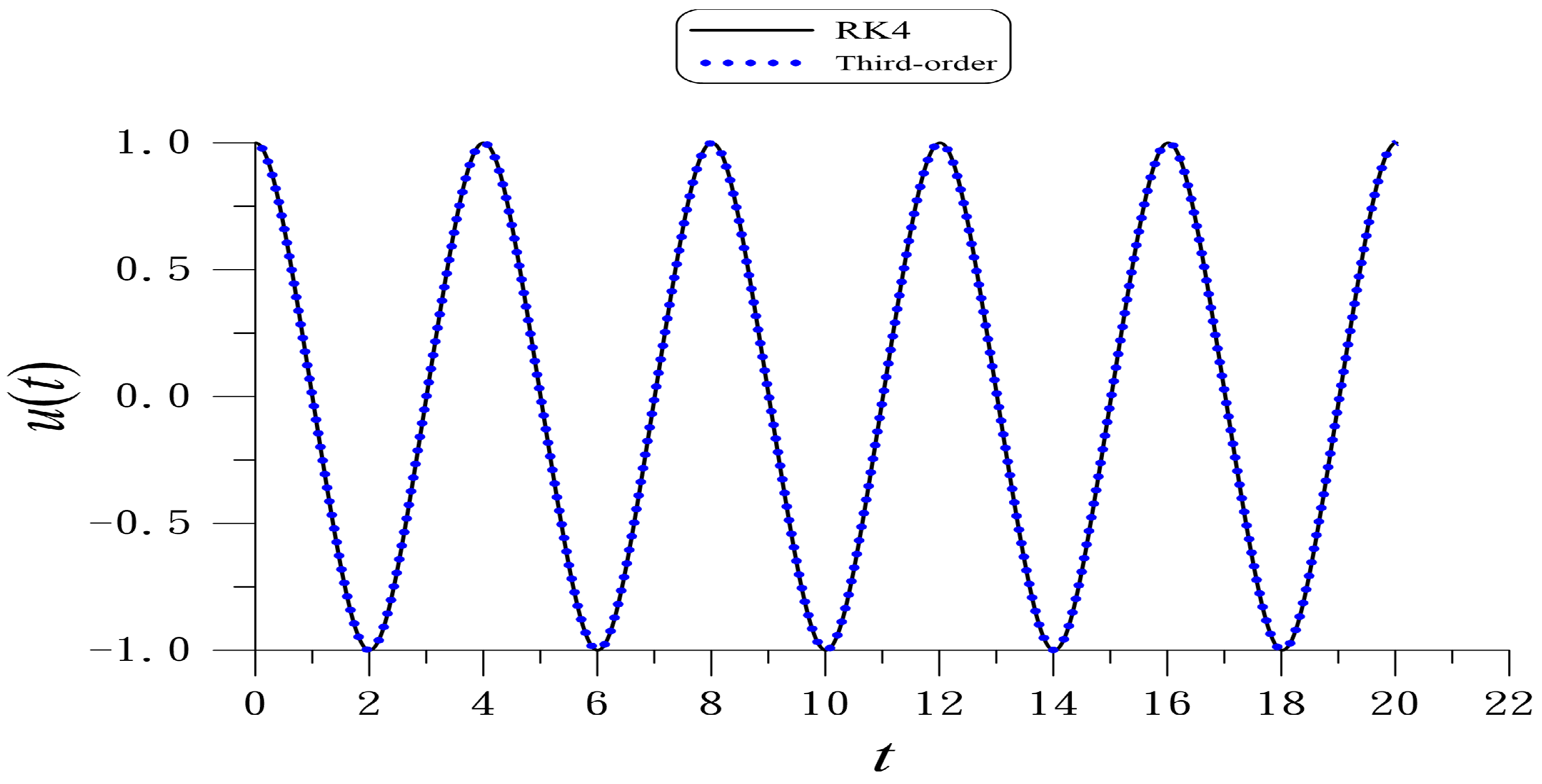
Given $A=1$, ${\epsilon }_0=2$, $\alpha =-0.017284$, and $q_0=3$, Figure 8 shows the third-order periodic solution within five periods compared to the RK4 solution, which is almost coincident with ME = $2.53\times {10}^{-4}$. Upon comparing the second-order periodic solution in Figure 7, a little improvement of the accuracy of the periodic solution from ME = $8.57\times {10}^{-4}$ to ME = $2.53\times {10}^{-4}$ is achieved.

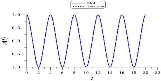
Figure 8. For the Duffing nonlinear oscillator within five periods comparing RK4 solution and the third-order periodic solution obtained from a hybrid method of the LRGM.

Remark 3.

We find that the algebraic manipulations to seek the third-order periodic solution becomes more complicated, but its accuracy upon comparing the second-order periodic solution is increased a little. Therefore, we suggest using the hybrid method together with the second-order periodic solution by using the LRGM to obtain the frequency and the analytic solution of the nonlinear oscillator.

10. Conclusions

This paper shed a new light on the ancient Chinese mathematics method used in He’s frequency–amplitude formula to estimate the frequency of a nonlinear oscillator. For a received new model of a nonlinear oscillator, if there exists no simple method to estimate the vibration frequency, He’s frequency–amplitude formula can produce a suitable approximation of the vibration frequency. Owing to this reason, He’s frequency–amplitude formula was employed by many researchers in their works to study the vibration behavior of the nonlinear oscillator.

The Chinese mathematics method was re-written as a fixed-point Newton form, and the equivalence of the Chinese mathematics method to the original nonlinear frequency equation was proven. We further modified the fixed-point Newton form by adding a term in the denominator to derive a new frequency–amplitude formula. We proposed a linearly perturbed frequency equation by adding a linear term in the original frequency equation. The new frequency formula obtained from the new frequency equation is more accurate than He’s frequency–amplitude formula, wherein the parameter involved in the new formula minimized the absolute error of the periodicity condition. The accuracy of the frequency obtained from the new frequency–amplitude formula and the linearly perturbed frequency equation can be significantly increased by several orders. Additionally, for He’s frequency–amplitude formula, if one attempts to obtain a highly precise value of the frequency for the newly received nonlinear oscillator, the new frequency–amplitude formula is a good candidate. We proposed the very simple linearized residual Galerkin method (LRGM) for seeking the second-order periodic solutions of nonlinear oscillators. A hybrid method was developed by combing the new frequency–amplitude formula to the LRGM to find the second-order analytic periodic solutions. Many examples were conducted to reveal that the proposed frequency–amplitude formula, linearly perturbed frequency equation, the LRGM and the hybrid method are highly efficient and accurate.

References

- Ismail, G.M.; Cveticanin, L. Higher order Hamiltonian approach for solving doubly clamped beam type N/MEMS subjected to the van der Waals attraction. Chin. J. Phys. 2021, 72, 69–77. [Google Scholar]
- Rehman, S.; Hussain, A.; Rahman, J.U.; Anjum, N.; Munir, T. Modified Laplace based variational iteration method for the mechanical vibrations and its applications. Acta Mech. Autom. 2022, 16, 98–102. [Google Scholar]
- Tang, W.; Anjum, N.; He, J.-H. Variational iteration method for the nanobeams-based N/MEMS system. MethodsX 2023, 11, 102465. [Google Scholar]
- Lu, J. Global residue harmonic balance method for strongly nonlinear oscillator with cubic and harmonic restoring force. J. Low Freq. Noise Vib. Active Control 2022, 41, 1402–1410. [Google Scholar]
- Wang, S.; Zhang, Y.; Guo, W.; Pi, T.; Li, X. Vibration analysis of nonlinear damping systems by the discrete incremental harmonic balance method. Nonlinear Dyn. 2023, 111, 2009–2028. [Google Scholar]
- Liu, C.S.; Kuo, C.L.; Chang, C.W. Linearized harmonic balance method for seeking the periodic vibrations of second and third orders nonlinear oscillators. Mathematics 2025, 13, 162. [Google Scholar] [CrossRef]
- Molla, M.; Sharif, N. Energy balance method for solving nonlinear oscillators with non-rational restoring force. Appl. Math. Sci. 2023, 17, 689–700. [Google Scholar]
- He, J.H.; Jiao, M.L.; Gepreel, K.A.; Khan, Y. Homotopy perturbation method for strongly nonlinear oscillators. Math. Comput. Simul. 2023, 204, 243–258. [Google Scholar]
- Ismail, G.M.; Abul-Ez, M.; Zayed, M.; Farea, N.M. Analytical accurate solutions of nonlinear oscillator systems via coupled homotopy-variational approach. Alex. Eng. J. 2022, 61, 5051–5058. [Google Scholar]
- Ismail, G.M.; El-Moshneb, M.M.; Zayed, M. Analytical technique for solving strongly nonlinear oscillator differential equations. Alex. Eng. J. 2023, 74, 547–557. [Google Scholar]
- Roy, Y.; Maiti, D.K. General approach on the best fitted linear operator and basis function for homotopy methods and application to strongly nonlinear oscillators. Math. Comput. Simul. 2024, 220, 44–64. [Google Scholar] [CrossRef]
- Mohammadian, M. Application of He’s new frequency-amplitude formulation for the nonlinear oscillators by introducing a new trend for determining the location points. Chin. J. Phys. 2024, 89, 1024–1040. [Google Scholar] [CrossRef]
- Ismail, G.M.; Kamel, A.; Alsarrani, A. Approximate analytical solutions to nonlinear oscillations via semi-analytical method. Alex. Eng. J. 2024, 98, 97–102. [Google Scholar] [CrossRef]
- He, J.H. Comment on He’s frequency formulation for nonlinear oscillators. Eur. J. Phys. 2008, 29, L19–L22. [Google Scholar] [CrossRef]
- He, J.H.; Garcia, A. The simplest amplitude-period formula for non-conservative oscillators. Rep. Mech. Eng. 2021, 2, 143–148. [Google Scholar] [CrossRef]
- Akbarzade, M.; Khan, Y. Dynamic model of large amplitude non-linear oscillations arising in the structural engineering: Analytical solutions. Math. Comput. Model. 2012, 55, 480–489. [Google Scholar] [CrossRef]
- Cai, X.C.; Liu, J.F. Application of the modified frequency formulation to a nonlinear oscillator. Comput. Math. Appl. 2011, 61, 2237–2240. [Google Scholar] [CrossRef]
- He, J.H. Amplitude-frequency relationship for conservative nonlinear oscillators with odd nonlinearities. Int. J. Appl. Comput. Math. 2017, 3, 1557–1560. [Google Scholar] [CrossRef]
- Ren, Z.F.; Hu, G.F. He’s frequency-amplitude formulation with average residuals for nonlinear oscillators. J. Low Freq. Noise Vib. Active Control 2018, 38, 1050–1059. [Google Scholar] [CrossRef]
- Wu, Y.; Liu, Y.P. Residual calculation in He’s frequency-amplitude formulation. J. Low Freq. Noise Vib. Active Control 2021, 40, 1040–1047. [Google Scholar] [CrossRef]
- Tian, D.; Liu, Z. Period/frequency estimation of a nonlinear oscillator. J. Low Freq. Noise Vib. Active Control 2019, 38, 1629–1634. [Google Scholar]
- He, C.H.; Wang, J.H.; Yao, S. A complement to period/frequency estimation of a nonlinear oscillator. J. Low Freq. Noise Vib. Active Control 2019, 38, 992–995. [Google Scholar]
- El-Dib, Y.O. A review of the frequency-amplitude formula for nonlinear oscillators and its advancements. J. Low Freq. Noise Vib. Active Control 2024, 43, 1032–1064. [Google Scholar]
- He, J.H. Ancient Chinese algorithm: The Ying Buzu Shu (method od surplus and deficiency) vs. Newton iteration method. Appl. Math. Mech. 2002, 23, 1407–1412. [Google Scholar]
- He, C.H. An introduction to an ancient Chinese algorithm and its modification. Int. J. Numer. Meth. Heat Fluid Flow 2016, 26, 2486–2491. [Google Scholar]
- Liu, Y.Q.; He, J.H. On relationship between two ancient Chinese algorithms and their application to flash evaporation. Results Phys. 2017, 7, 320–322. [Google Scholar]
- Liu, C.S.; Chang, C.W. Updating to optimal parametric values by memory-dependent methods: Fractional type iterative schemes for solving nonlinear equations. Mathematics 2024, 12, 1032. [Google Scholar]
- He, C.H.; He, J.H. Double trials method for nonlinear problems arising in heat transfer. Therm. Sci. Suppl. 2011, 15, S153–S155. [Google Scholar]
- Krasnosel’skii, M.A.; Vainikko, G.M.; Zabreiko, P.P.; Rutitcki, J.B.; Stecenko, V.J. Approximated Solutions of Operator Equations; Walters–Noordhoff: Groningen, The Netherlands, 1972. [Google Scholar]
- Fatoorehchi, H.; Abolghasemi, H.; Rach, R. A new parametric algorithm for isothermal flash calculations by the Adomian decomposition of Michaelis-Menten type nonlinearities. Fluid Phase Equilib. 2015, 395, 44–50. [Google Scholar] [CrossRef]
- He, J.H. Some asymptotic methods for strongly nonlinear equations. Int. J. Modern Phy. B 2006, 20, 1141–1199. [Google Scholar] [CrossRef]
- Geng, L.; Cai, X.C. He’s frequency formulation for nonlinear oscillators. Eur. J. Phys. 2007, 28, 923–931. [Google Scholar]
- Ren, Z.F.; Gui, W.K. He’s frequency formulation for nonlinear oscillators using a golden mean location. Comput. Math. Appl. 2011, 61, 1987–1990. [Google Scholar]
- Mickens, R.E. Investigation of the properties of the period for the nonlinear oscillator x¨+(1+x˙2)x=0. J. Sound Vib. 2006, 292, 1031–1035. [Google Scholar]
- Liu, C.S.; Chang, C.W. A novel perturbation method to approximate the solution of nonlinear ordinary differential equation after being linearized to the Mathieu equation. Mech. Syst. Signal Process. 2022, 178, 109261. [Google Scholar]
- He, J.H. Modified Lindstedt-Poincare methods for some strongly nonlinear oscillations Part I: Expansion of a constant. Int. J. Non-Linear Mech. 2002, 37, 309–314. [Google Scholar]
- Shou, D.H. The homotopy perturbation method for nonlinear oscillators. Comput. Math. Appl. 2009, 58, 2456–2459. [Google Scholar]
- Zhao, L. He’s frequency-amplitude formulation for nonlinear oscillators with an irrational force. Comput. Math. Appl. 2009, 58, 2477–2479. [Google Scholar]
- Ren, Z.F.; Wu, J.B. He’s frequency-amplitude formulation for nonlinear oscillator with damping. J. Low Freq. Noise Vib. Active Control 2019, 38, 1045–1049. [Google Scholar]
- Yao, S.W.; Cheng, Z.B. The homotopy perturbation method for a nonlinear oscillator with a damping. J. Low Freq. Noise Vib. Active Control 2019, 38, 1110–1112. [Google Scholar]
- Ma, H. Simplified Hamiltonian-based frequency-amplitude formulation for nonlinear vibration systems. Facta Univ. Ser. Mech. Eng. 2022, 20, 445–455. [Google Scholar]
- He, J.H.; Hou, W.F.; Qie, N.; Gepreel, A.K.; Shirazi, A.H.; Sedighi, H.M. Hamiltonian-based frequency-amplitude formulation for nonlinear oscillators. Facta-Univ.-Ser. Mech. Eng. 2021, 19, 199–208. [Google Scholar] [CrossRef]
- El-Dib, Y.O. Insightful and comprehensive formularization of frequency–amplitude formula for strong or singular nonlinear oscillators. J. Low Freq. Noise Vib. Active Control 2023, 42, 89–109. [Google Scholar] [CrossRef]
- El-Dib, Y.O.; Alyousef, H.A. Successive approximate solutions for nonlinear oscillation and improvement of the solution accuracy with efficient non-perturbative technique. J. Low Freq. Noise Vib. Active Control 2023, 42, 1296–1311. [Google Scholar] [CrossRef]
- Leung, A.Y.T.; Guo, Z. Homotopy perturbation for conservative Helmholtz-Duffing oscillators. J. Sound Vib. 2009, 325, 287–296. [Google Scholar] [CrossRef]
- Askari, H.; Saadatnia, Z.; Younesian, D.; Yildirim, A.; Kalami-Yazdi, M. Approximate periodic solutions for the Helmholtz–Duffing equation. Comput. Math. Appl. 2011, 62, 3894–3901. [Google Scholar] [CrossRef]
Disclaimer/Publisher’s Note: The statements, opinions and data contained in all publications are solely those of the individual author(s) and contributor(s) and not of MDPI and/or the editor(s). MDPI and/or the editor(s) disclaim responsibility for any injury to people or property resulting from any ideas, methods, instructions or products referred to in the content. |
© 2025 by the authors. Licensee MDPI, Basel, Switzerland. This article is an open access article distributed under the terms and conditions of the Creative Commons Attribution (CC BY) license (https://creativecommons.org/licenses/by/4.0/).