1. Introduction
The European Union’s Green Paper specifies the need to substitute 20% of conventional fuel consumption with alternative fuels by the year 2020. An alternative energy source (not considering electricity) is natural gas (NG) that is relatively one of the most environmentally friendly as it has an inherently clean combustion process [
1]. Natural gas is transported from gas fields to distribution-network systems in two main ways, either by pipeline or by ships in the form of liquefied natural gas (LNG).
LNG is produced by cooling natural gas below its boiling point (
°C at ambient pressure) at the liquefaction plant located nearby the gas-production source. LNG is transported from production site to receiving terminals through special ships (LNG tankers) that keep LNG in a liquid phase. After the regasification procedure, the gas is input into a local gas-pipeline network. However, recently, some small-scale LNG (SSLNG) facilities have emerged with regional storage hubs and direct gas supply. LNG is transported from the terminal to satellite terminals by smaller LNG ships or trucks. Such terminals are used for receiving and storing LNG for a limited period of time depending on storage capacity. Their capacity ranges from a couple of hundred of m
to around 20 m
. The SSLNG market is developing rapidly, especially for transportation fuel, and to serve end users in remote areas or those that are not connected to the main pipeline infrastructure [
2]. In the case of Spain, six regasification terminals are in operation, in Barcelona, Sagunto, Cartagena, Huelva, Bilbao, and Mugardos. In 2015, 869 sites received LNG with a fleet of approximately 35,000 trucks. The largest is Barcelona with 232 destinations [
3,
4]. Thus, the supply chain is one of the main problems of SSLNG satellite terminals. In this case, small-scale supply-chain natural gas must be transported from a large import terminal to consumers through a network of smaller satellite terminals with truck transports. LNG carriers used in this type of system have smaller capacities and must perform multistep voyages.
Supply-chain planning consists of designing an optimal and feasible distribution plan for the whole supply chain. In the case of satellite terminals, the supply chain must take into account LNG consumption in order to guarantee its safety storage. Since gas consumption strongly fluctuates and follows the weather changes of different seasons, making a good plan is not easy, and even less so in the case of satellite LNG for domestic users.
Improved information is key for making decisions to guarantee safety operations of LNG regasification satellite plants. Therefore, this paper proposes to predict the remaining time by providing remaining useful life (RUL) to refill the LNG tanks that is very useful for the predictive-maintenance plan of the LNG satellite plants, and for applying the optimal management of a truck service to refill LNG tanks when a company has many plants working simultaneously in the region.
The article is structured as follows: In
Section 2, we present the related work.
Section 3 describes the problem under study.
Section 4 is dedicated to the description of methodologies used for solving the problem.
Section 5 shows detailed experiment results and comparisons. Finally, conclusions are given in
Section 6.
2. Related Work
In the last decade, the number of publications regarding LNG supply chains have increased. Bittante et al. [
5] presented a mixed-integer linear-programming (MILP) model for the optimal design of a supply chain for a problem where NG is distributed from a set of potential suppliers to a set of consumers using a heterogeneous fleet of ships. Jokienen et al. [
6], presented an MILP model for small-scale LNG supply chain optimization for supply along a coastline, minimizing the costs related to fuel procurement and providing optimal supply-chain configuration with regard to satellite-port locations, ship sizes, and customer demand. In the two cases presented above, LNG consumer demands must be known or accurately predicted.
On the other hand, the prediction of natural gas consumption is indispensable for efficient system operation, and required for planning decisions at local distribution companies of natural gas. Researchers attempted to develop models for the prediction of NG consumption on a short-term (from 30 min to a week), medium-term (from a month to two years), and long-term (3–20 years) basis using mathematical and computational techniques. An extended overview of the published papers in the area of forecasting NG consumption can be found in [
7,
8,
9,
10].
It is remarkable that the majority of prediction models were developed considering different types and numbers of input variables. Özmen et al. [
11] used data-driven method multivariate adaptive regression splines (MARS) to determine the optimal combination of basic functions. Their proposed model included sixteen variables, among which maximal and medium temperature, price, and number of users. Soldo et al. [
12] investigated the influence of solar radiation on improving NG consumption forecasting models. Beyca et al. [
13] employed multiple linear regression (MLR), an artificial-neural-network approach (ANN), and support vector regression (SVR) for the forecasting of NG consumption in the province of Istanbul. The study indicated that SVR was far superior to the ANN technique, providing more reliable and accurate results in terms of lower prediction errors for time-series forecasting of natural gas consumption.
The aforementioned methods use multivariate models that include natural gas consumption, meteorological data, seasonal trends, price of natural gas, population, among others, with an increase of data-collection difficulty. To solve this problem, the authors in [
14] proposed a sensor-data-driven model based only on the time series of the NG consumption, presenting a structure-calibrated support-vector-regression (SC-SVR) approach for forecasting daily NG consumption that is correlated with past time series using the SVR model. The calibration of the structural parameters for the next-day forecast is performed by an extended Kalman filter. Laib et al. [
15] described the current state of the art and proposed an adaptive hybrid architecture based on a long short-term memory (LSTM) recurrent model for predicting efficiently the NG consumption, and a multilayered perceptron (MLP) neural network for estimating daily consumption. Akpinar et al. [
16] studied time series decomposition, Holt-Winters exponential smoothing and autoregressive integrated moving average (ARIMA) methods, the models proposed includes seasonal and trends components and are applied for the monthly demand prediction of NG. Bose et al. [
17] reviewed the contribution in the area of Fuzzy time series (FTS) forecasting, these models have proven to be a powerful tool for modelling and forecasting complex systems in different domains including energy, economics, biology, etc. One of this technique is the Fuzzy Inductive Reasoning (FIR), which has used for energy forecasting in residential buildings and smart grid [
18,
19].
The consumption forecast plays an important role in predicting LNG storage evolution. In this regard, predicting the storage level allows to know if a consumer’s demand for a time period can be satisfied while guaranteeing safety levels. The problem of predicting or forecasting the future evolution of the storage level can be solved by using prognosis algorithms. In the prognostics literature, the concept of remaining useful life (RUL) appeared, defined as the time from the current instant to the time of end of life. Reliable RUL predictions provide valuable information for condition-based maintenance, thus improving LNG regasification terminal performance. Prognostics plays an important role in health-management systems and have been used for predicting the RUL for plant equipment, such as compressors [
20], pipelines [
21], and pumps [
22], a reviewed of the main approaches to Prognostics and Health Management (PHM) and to predict RUL can be found in [
23]. The single and double exponential smoothing method are currently one of the most popular time series forecast methods and had been successfully applied in diverse fields such as water quality [
24], air quality index [
25], petroleum demand [
26], among others.
As in the case of consumption prediction, prognosis has been implemented using approaches that are data-driven, physics-based, or hybrid approaches [
27]. During prognosis and health-management (PHM) analysis, historical knowledge carried by data is systematically fed into a decision-making process by sophisticated data modelling techniques [
28]. However, it is frequently observed that collected (raw) data are redundant, incomplete, or inaccurate, as well as heterogeneous and false due to faulty sensors [
29]. For this reason, PHM contains four main components: data processing, feature extraction, fault diagnosis, and failure prognosis [
30].
The methods for consumption prediction or LNG storage prediction may produce satisfactory results depending on data availability. In general, the sensor-data validation process consists of two main steps: faulty-sensor-data detection and correction or data reconciliation. Faulty-sensor-data detection identifies incorrect values in the sensor data, and the correction process provides methods to deal with incoherent sensor data. In each category, a number of different tools and methods exist, a exhaustive review of these techniques can be found in [
31]. There is no perfect or universal tool for this task, and the success of the considered approach depends on a number of factors, such as the type of monitored variable, overall measurement conditions, the used sensor, and the characteristics of the phenomenon being captured. Most of these methods are difficult to perform with asynchronous so it is desirable to convert them to uniform sampled data using resampling algorithms. For example, in [
32], two algorithms were proposed for an asynchronous-to-synchronous resampling scheme. Signal resampling is one of the steps of the data-preprocessing process, used in many applications, such as prognosis and health management (e.g., [
33]) and state identification (e.g., [
34]).
3. Problem Description
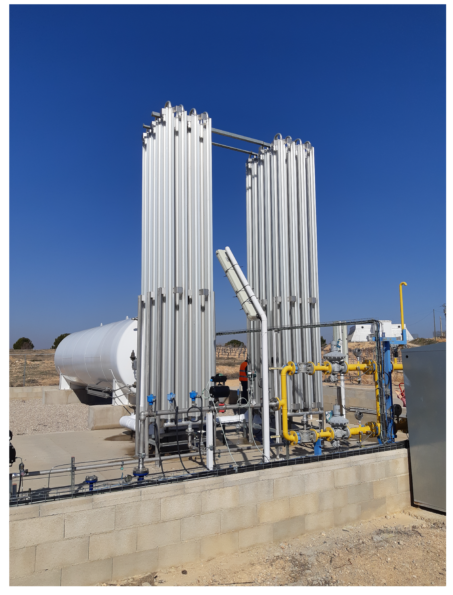
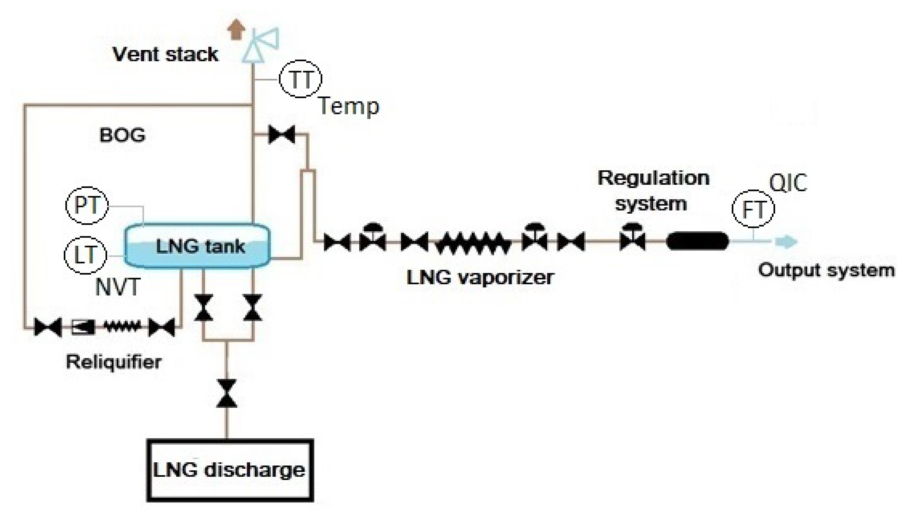
A regasification LNG satellite plant (
Figure 1) is composed of the following systems for its operation (
Figure 2):
- a)
LNG discharge: Allows to carry out LNG transfer between tanker trucks and storage tanks.
- b)
Storage: integrated by one or more double containment tanks, used for storing LNG at cryogenic temperatures.
- c)
LNG vaporizer: An uncomplicated heat exchanger that vaporizes liquefied gas by using heat absorbed from ambient air.
- d)
Regulation system: Reduces and establishes gas pressure for the supply through the distribution network.
- e)
Control system and plant operation: Maintains the control of the system in all its operating parameters, with emergency stops that allow it to immediately cut the supply in case of an emergency.
In LNG storage tanks, gas is generated such that, if not extracted, it accumulates in the tank causing pressure to rise. The main causes of this gas generation are due to:
Vaporizing the LNG contained in the tank due to the exchange of heat with the outside through the walls and roof of the tank. Storage temperature is °C, and, although the tank is cryogenic with two containers and important insulation in the chamber between them, there is a certain level of heat exchange, causing an increase in the tank temperature and moving the equilibrium point towards a higher pressure.
Compressing the gas in equilibrium with the stored LNG during tank filling by trucks.
The gas generated in excess regarding the amount of gas in equilibrium with LNG, known as boil-off gas (BOG), has to be evacuated from the tanks through vent stacks (see
Figure 2) to maintain stable pressure in the tanks.
The BOG is recovered by a reliquifier and is mainly reintroduced in liquid phase into the tank to avoid product loss at the plant exit and unnecessary gas emissions into the atmosphere, avoiding a negative impact to the environment.
The reliquifier is pressurized equipment in which gases coming from the boil-off come in contact with the subcooled LNG coming from the storage tank for its condensation.
The regasification system heats the LNG from the tank. Then, the outflow of liquid from the tank decreases the level inside and increases the volume occupied by the gas phase at the top. Since the tank is thermally insulated, there is no vaporization of liquid to gas, so pressure of the gas phase decreases by increasing the volume it occupies. To maintain gas pressure and prevent its lowering, there is a regulator called rapid pressure setting (PPR) that controls the regasification of the extracted liquid gas from the tank in a closed circuit.
The operation of the system is controlled by a programmable logic controller (PLC) that can acquire sensor values and command actuators. Sensor data are collected in PLCs and transmitted to a SCADA system, and data are stored in a database system based on a mechanism that combines a time-triggered period of one hour with an event-triggered approach. In turn, this means that each stored variable has its own mean sampling time.
Figure 3 shows the time evolution of pressure (PT) and level (NVT) inside the tank, NG consumption, and ambient temperature of one year in one of the analyzed satellite plants. Pressure is controlled around 3–4 bar, and LNG level decreases by regasification consumption and refilling by LNG transfer between tanker trucks and storage tanks. In the middle of the year (mainly summer with a higher temperature), level drops are smoother because of a reduction in consumption.
Two problems are addressed in this paper. First, validating raw sensor data and, in case that the data are not consistent, try to provide estimations that allow to reconstruct the complete database. Therefore, the first objective is to transform raw data into reliable and safe information of the system so that they can be used in fault diagnosis, prognosis, and for the control and optimal management of LNG regasification satellite plants. The second objective is to develop a new methodology for the prognosis of remaining useful life to refill of LNG the tank of the plant and to compare it with one of the popular time series forecasting methods. The new methodology is based on fuzzy inductive reasoning using historical data for model training.
4. Methodology
4.1. Sensor-Data Validation and Reconstruction
Collected data in satellite terminals are sent to a remote central server where they are stored. These data are useful for remote meter reading, monitoring consumption, and controlling. Unfortunately, the stored data suffer from problems such as missing and spurious values, and duplicate records. For decreasing the volume of transmitted data, the monitoring strategy is an event- and time-based method (with a sample time of 1 h), leading to asynchronous and nonuniform sampled signals. Before use, it is necessary to to ensure data quality. Our methodology works offline and, following the method proposed in [
35], it combines signal processing techniques with spatial models allowing to validate and reconstruct missing and false data. It consists of the following steps:
Step 0 (obtain variable values): Data are exported from the plant database as a .txt file. Each text line includes metadata such as event date and time, satellite-plant identification, and variable name and value. The initial step is to obtain the value of the variables, and to convert date–time information to an ISO format. Each variable is stored in a separate file.
Step 1 (duplicated-record detection): duplicated records are detected using time information and removed.
Step 2 (physical-range limits and equipment state): This step checks whether data are within the physical range of the sensor acquiring corresponding measurement. The expected range of the measurements may be obtained from sensor specifications or historical data records. It also allows to check the consistency of the variables in a given equipment unit, i.e., sensor or actuator.
Step 3 (resampling data): As data are asymmetric, resampling allows to construct a periodical series of new samples on the basis of the original dataset. Resampling is performed by using linear interpolation between nearest-neighbor data. Sampling time is selected on the basis of the minimal time between two consecutive events.
Step 4 (trend level): Checks whether data are derivative, i.e., if the magnitude change of the data in consecutive sample times is within their expected rate. This allows detecting unexpected and possibly undesired sudden changes in the data.
Step 5 (spatial model): Checks the consistency of collected data by a certain sensor with its spatial model, i.e., correlation between data coming from spatially related sensors. This spatial model is obtained from the physical relations among the plant variables.
4.2. Sensor-Data-Driven Prognosis Methods
The sensor-data-driven prognosis approach proposes forecasting the RUL on the basis of a predetermined end-of-life or failure threshold (FT). As proposed in [
36,
37], the RUL is given by:
where
is the RUL step-ahead forecast at the sampled
k of a given predictive model.
A sensor-data-driven approach is used to derive the predictive models from the collected data. We propose a new method based on fuzzy-inductive-reasoning model for multistep forecast of the tank-storage level. This new methodology is compared with the Brown’s double exponential smoothing method.
4.2.1. Fuzzy-Inductive-Reasoning Methodology
Fuzzy-inductive-reasoning (FIR) methodology is a sensor-data-driven approach based on general systems theory proposed by [
38]. It is a modelling and qualitative-simulation methodology that allows to obtain qualitative relations between variables that compose a system, and to infer its future behavior. It can also describe systems that cannot easily be described by classical mathematics (e.g., differential equations), that is, systems for which underlying physical laws are not well-understood. FIR consists of four main processes, namely, fuzzification, qualitative model identification, fuzzy forecast, and defuzzification [
39,
40].
The fuzzification process converts quantitative data obtained from the system into fuzzy data that consist of a triplet containing class, membership, and side values.
The qualitative-model identification process is responsible for finding causal and temporal relations between variables, therefore allowing to obtain the best model (or optimal mask) that represents the system. The optimal mask is selected from a candidate matrix using quality criteria.
Once the FIR model is available, a prediction can be performed using the FIR inference engine, called the fuzzy-forecast process, which is a specialization of the k-nearest-neighbor rule commonly used in the pattern-recognition field.
Finally, defuzzification is the inverse process of fuzzification. It allows converting the qualitative predicted output into quantitative values that can then be used as inputs to an external quantitative model.
For better understanding,
Table 1 shows an example of a mask with a depth of 2 (2-depth). Each column corresponds to one variable, and each row corresponds to mask depth or the causal-time relation between variables, where
k is the sample time. The negative elements is called
m-input (mask input) (enumeration of m-inputs in the optimal mask has no relevance). The single positive value denotes the m-output. In this example, the mask is equivalent to the causal relation given by
with
representing the fuzzy-inductive-reasoning function and
the predicted value. The optimal mask is obtained from a candidate mask performing exhaustive research; checking with of them allows to obtain the best quality criteria.
Assuming that n is the mask depth, the causal relation can be represented by , where is a window of known inputs, and is a window of past outputs considering samples from to k.
The FIR model can be used to forecast the RUL only in case the
input is either known in advance or can be estimated (or predicted). Given initial time
, horizon of prediction
h, and function
g that allow to calculate future input values
with
, the RUL can be computed following Algorithm 1. This computes the predicted state using the FIR model in simulation, and the RUL is determined when the predicted state reaches the predefined failure threshold (FT).
| Algorithm 1: Remaining useful life (RUL) forecast with a fuzzy-inductive-reasoning (FIR) model |
 |
4.2.2. Brown’s Double-Exponential-Smoothing Method
Brown’s double exponential smoothing, also known as Brown’s linear exponential smoothing, is a type of double exponential smoothing that uses two different smoothed series that are centered at different points in time [
41]. The method is based on the extrapolation of a line through two centers, as presented below.
where
denotes the single-smoothed series obtained by applying simple exponential smoothing to series
y,
denotes the double-smoothed series obtained by applying simple exponential smoothing to series
, and
is the smoothing parameter.
Then, predicted
on an
horizon is computed by
where
ℓ denotes an estimate of the level of the series at time
k, and
b denotes an estimation of the slope (or growth) of the series at time
k,
In practice, due to noise in the measurements, the predicted values have uncertainty. For considering this uncertainty in
, a confidence interval of 5% was included in Equation (
4).
From Equation (
4), we can also derive the estimated time for reaching a particular position. For instance, considering value
, estimated time
to reach this value is computed by:
5. Application to Predictive Maintenance of LNG Tank Refilling by Means of Trucks
The problem formulated in
Section 3 is solved in two phases: The first deals with data processing, and the second phase builds a prognostic model for determining the remaining time for refilling in the LNG tank. The second phase is solved by using the two methodologies explained below. The FIR methodology uses annual mean temperature to predict the tank-emptying time, while the Brown method uses tank-level evolution.
5.1. Sensor-Data-Processing Task
Raw data stored in the database are analyzed following the data validation and reconstruction procedure described in
Section 4.1. This procedure ensures data reliability for further decision-making. In this section, we explain the procedure for deriving one of the spatial models.
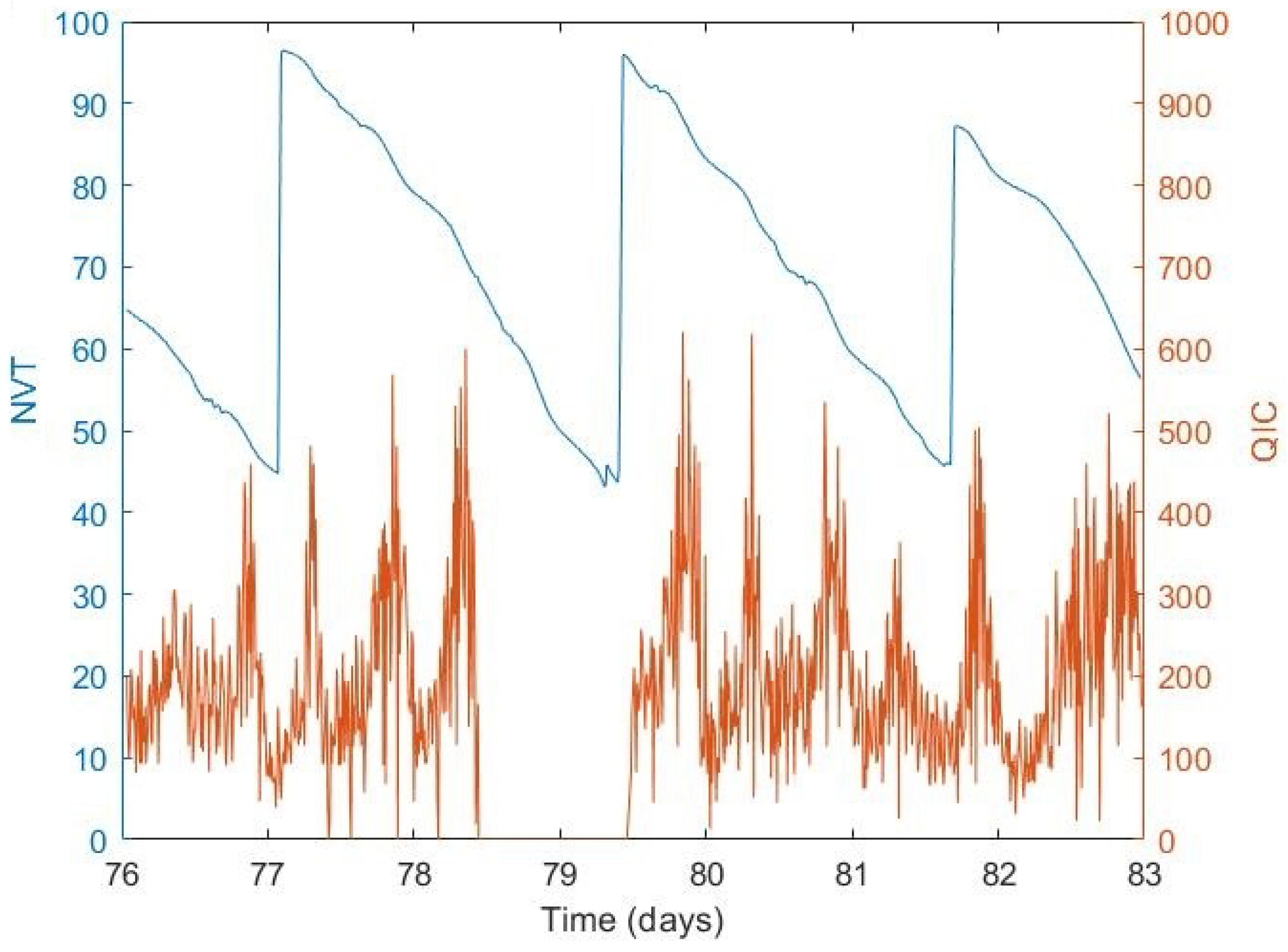
Figure 4 shows the time evolution of gas consumption (measured by flowmeter, QIC) and the level of LNG (NVT) in the storage tank of a satellite plant during several days of March 2018 after resampling with a sampled time of 10 min. There was discrepancy between the QIC flow sensor and the tank level in interval days 78 to 80, while the flow sensor indicated a zero value when tank level decreased. This anomalous behavior could not be detected by using Steps 2 to 4 presented in
Section 4.1 because, in summer, gas consumption could be zero and remains in this state for several hours. This figure also shows that the tank level had cyclical behavior; after finishing the truck discharge, the tank level was at its maximum, and it decreased with consumption.
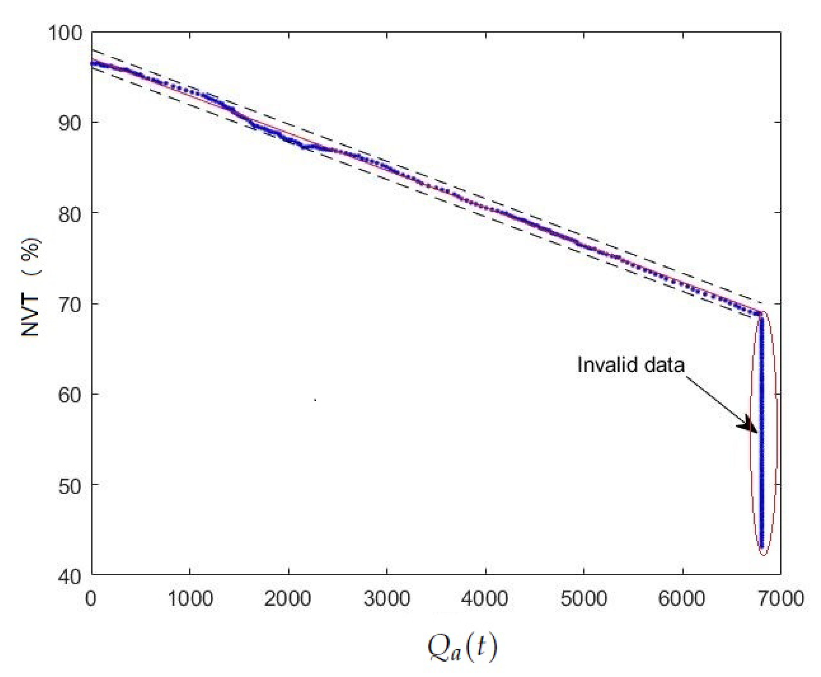
Using Step 5 (spatial-model test) of the methodology presented in
Section 4.1, when correlating the integral of gas-flow consumption between two refilling operations with the LNG tank level, ia relationship was observed given by the constant of liquid-to-gas conversion (
K = 244). This is shown in the XY plot of
Figure 5, where the blue continuous line corresponds to the correlation between the integral of gas-flow consumption and LNG tank level in 19–20 March 2018, and the red continuous line is calculated by
where
is the estimated level,
the initial tank value,
K the liquid-to natural gas conversion constant in normal conditions,
is the time between two refilling operations,
q the natural gas consumption, and
the accumulated natural gas consumption. Finally, the black discontinuous bands show the estimated uncertainties. This spatial model is also useful to reconstruct the wrong data provided by the flowmeter sensor. This spatial model could be useful if faulty data appear in the LNG level in the tank. In this case, gas consumption could be used to reconstruct level data.
5.2. Prognosis of Remaining Time to Refill Tank Using FIR Methodology
Weather (mainly temperature) is one of the most important factors that influences daily urban gas consumption. Using the FIR methodology described in
Section 4.2.1, we obtained a model for simulating gas consumption per operation-tank cycle using mean annual temperature.
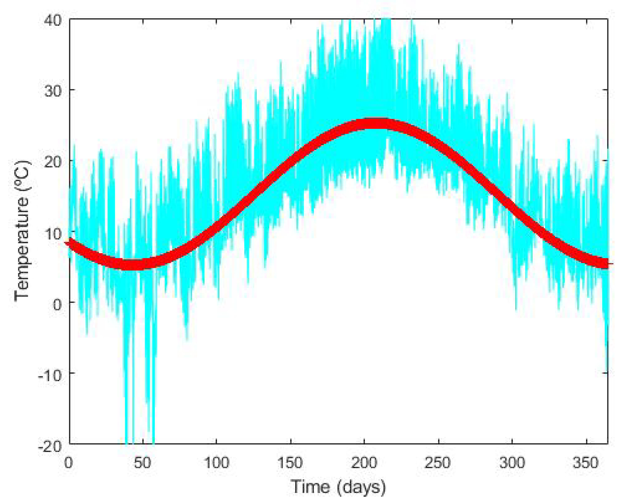
In a satellite plant, temperature is an important parameter related with its safety. For this purpose, the plant is equipped with several temperature sensors. There is a temperature sensor for detecting tank depressurization (or venting emissions); in normal operation, this sensor measures ambient temperature.
Figure 6 shows in the cyan line the data of this sensor during 2018.
Mean ambient temperature (
) of the whole period is approximated by Fourier series representation
in which the parameters are fitted to the data using a nonlinear least-squares algorithm.
Figure 6 shows the values of
in red line, with estimate parameters
= 15.26,
= −6.789,
= −7.321, and
w = 0.019.
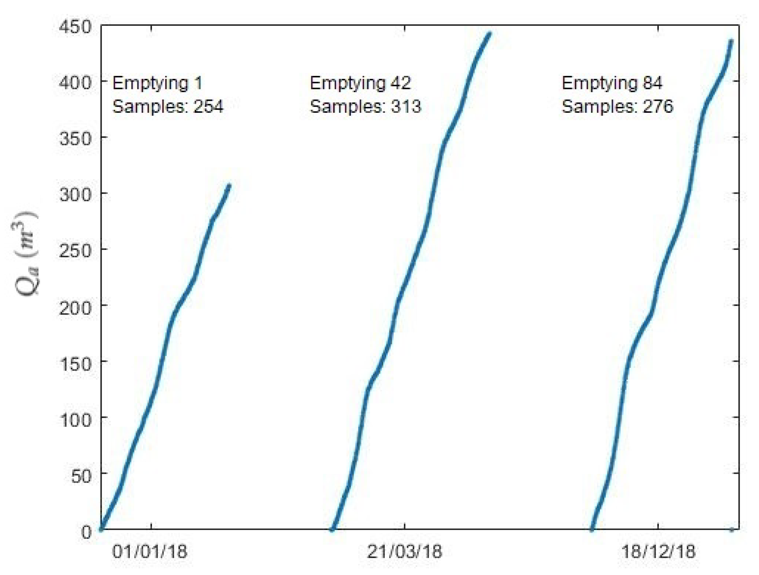
In order to obtain FIR models, it is necessary to define two parameters: The first is related to the fuzzification process of the variables (number of classes per variable) and the membership function, as was described in
Section 4.2.1. In our case, there were two variables,
is the temporal series given by Equation (
10), and
is the accumulated consumption given by Equation (
8). Data were divided into 84 datasets corresponding with the time intervals between refilling;
Figure 7 shows three of them. In this application, variables were discretized into three classes, and the equal-frequency-partition method was used to determine the membership function of the classes.
The proposed candidate mask is displayed in
Table 2. The two columns are associated with variables,
and
, and the rows with their samples. The proposed mask had a depth of one day, resulting a candidate mask of depth-144, since the variable sequences were sampled every 10 min. In order to reduce the computation complexity and enable fast convergence to an optimal mask, in the
input of the candidate mask, only one sample per hour was considered. It can be observed in
Table 2, where
is equal to −1 for
; otherwise, it is zero. The candidate mask assumed a causal relation between the two variables each hour during one day.
The found optimal mask had causal relation , which means that the consumption prediction at instant k, depends on the consumption of samples 6, 78, and 114 before, which is equivalent to 1, 13, and 19 h, and the temperature of 144 samples (or 24 h) before.
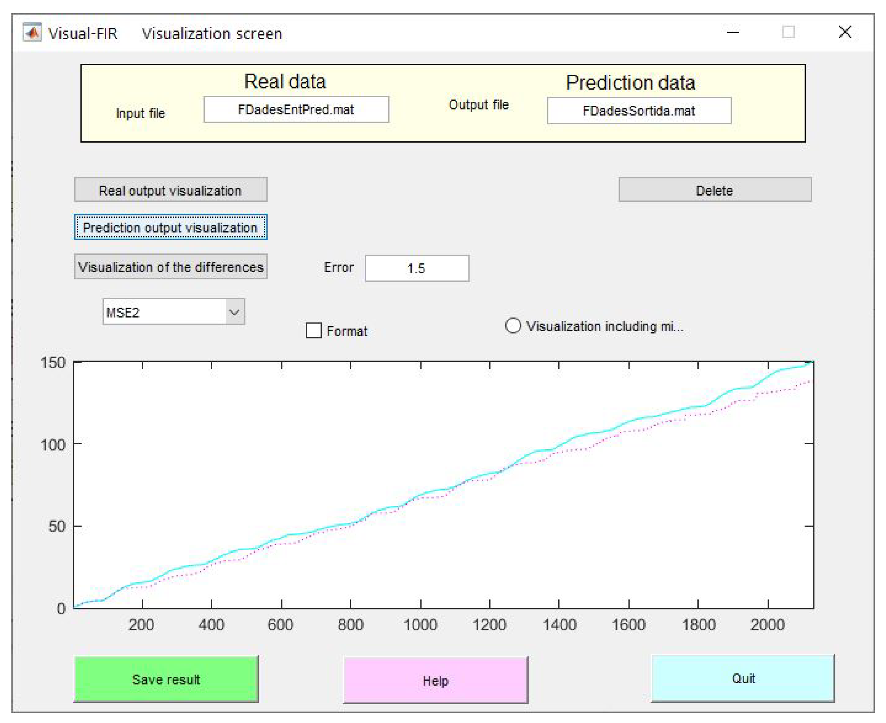
The whole available datasets were divided into training and evaluating sets. First, 68 datasets were used for training the model, and the remaining 16 datasets for evaluating the performance of the prediction model.
Figure 8 shows the Visual FIR main screen where we can visualize the real output signal (blue), the predicted signal (red dashed line), and the mean square error (MSE2).
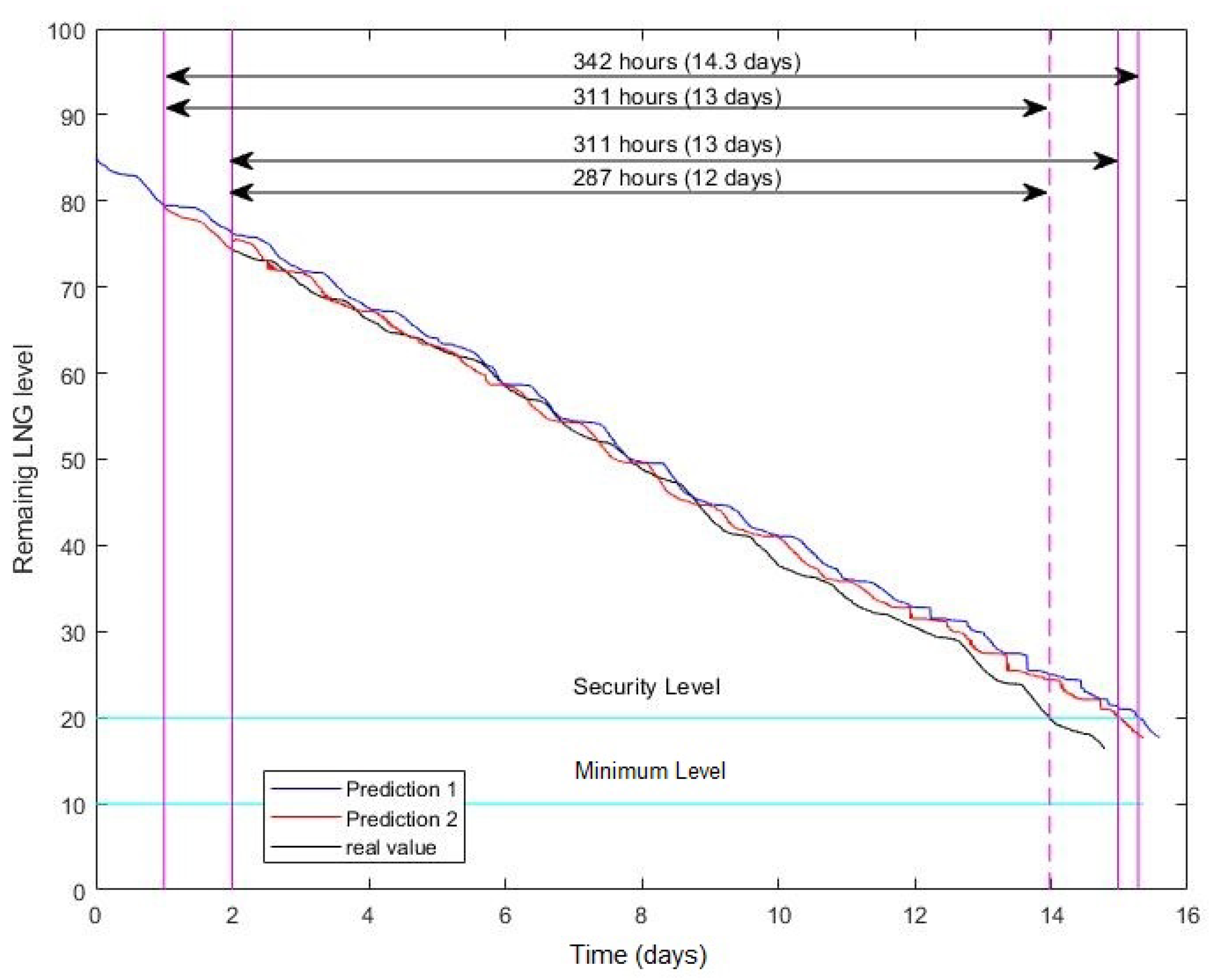
The estimated model was used recursively for predicting the tank-emptying time. The tank level was computed as
where
is the estimation of the accumulated consumption computed by the FIR model.
Figure 9 presents the decreasing tank level (black line), and the prediction level on the
day (24 h; blue line) and on
days (48 h; red line). In this study, we were interested in computing the RUL until the tank level reached its safety threshold, which meant an NVT of 20%. To this aim, we used Algorithm 1 with the following data:
days,
,
, which is a set given by
, and
= 20. The first prediction gave an RUL of 342 h, while the second provided an RUL value of 311 h. Comparing with the real data, the prediction errors in the first and second prediction were 31 and 24 h, respectively. The RUL was calculated dynamically using the new observations obtained from the online monitoring system. It is possible to consider other safety indicators, for example, remaining time until the tank level reaches its minimal threshold.
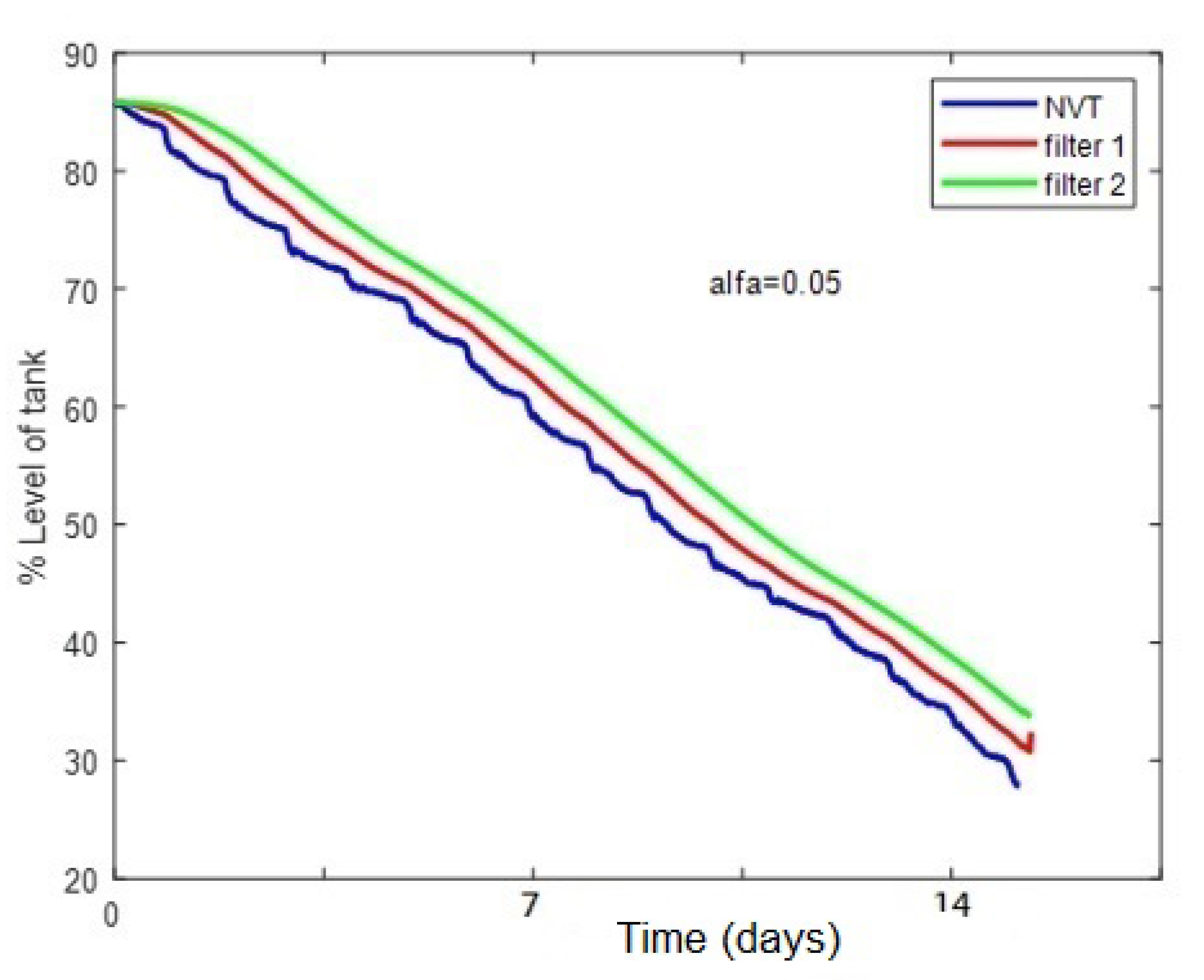
5.3. Prognosis of Remaining Time to Refill Tank Using Brown’S Double-Filter Method
The double aliasing of Brown, explained in
Section 4.2.2, is very useful for the prognosis of the remaining time to refill the tank.
Figure 10 shows the temporal pattern of the decreasing level in the blue line, and the two filtered signals,
in red and
in green, with a prefixed parameter
= 0.05.
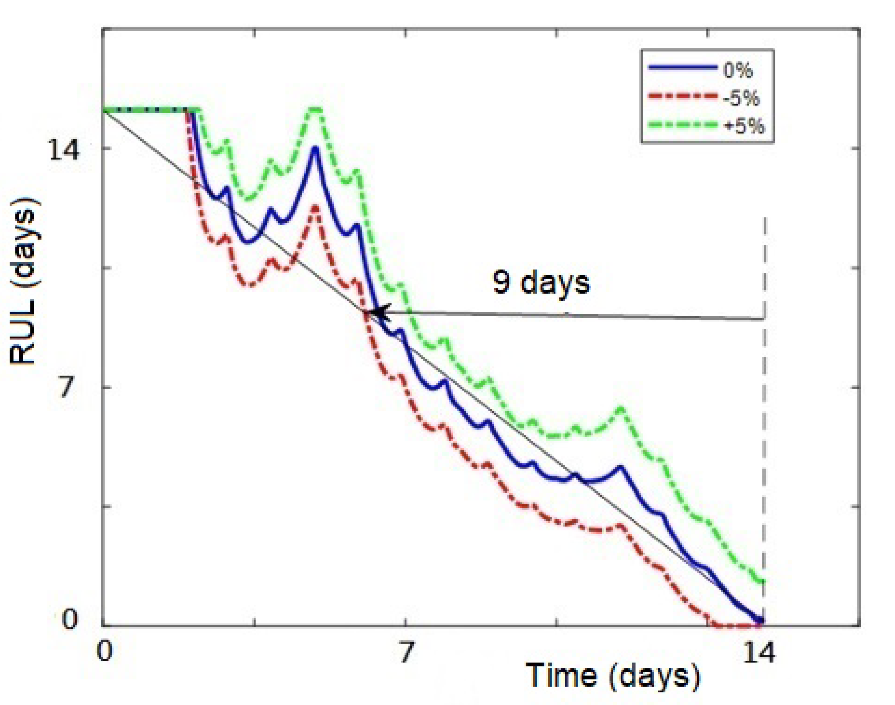
Figure 11 shows remaining useful time
to achieve the minimal level in the tank in the blue line, with a confidence interval of +/−5%, in the red and green line, respectively. The results showed that Brown’s algorithm can predict the situation of achieving the minimal tank level in 9 days. Reliable remaining useful time obtained in this scenario is 9 days, practically 50% of the time needed to empty the tank. This result is useful information to outline the process for. managing a request for a new tank refill. Comparing the Brown double-aliasing method of prognosis with the FIR method for the same scenario, both were both quite good, with 9 and 14 days of anticipation time, respectively, but the FIR method gave better anticipation of days. The same results were obtained for other scenarios, and this better performance of FIR is quite reasonable because it is a nonlinear method, uses other variables such as tank temperature, and it needs a learning period of data to produce good results. Brown double aliasing is a linear method but it does not need any extra information (e.g., temperature) or any learning period of data. Similar results were obtained in any period of the year, but time anticipation was always around 50% of the cycle, which allows to predict with a minimum of days to achieve the minimal tank level, this being useful information for a predictive-maintenance plan to refill the tank by means of trucks.
6. Conclusions
The objective of LNG satellite plants is to continuously supply gas to remote geographical areas. Due to the small size of the tanks in these plants, usually 20, 30, or 60 m, emptying frequency is between two and four days in winter. For this reason, a key strategy for continuously maintaining the level of the plant is to implement predictive plans to refill tanks with LNG via trucks.
First, this work addressed the problem of transforming aperiodic raw data based on events into periodic and validated/reconstructed data. For this, a data-validation methodology was proposed on the basis of a set of tests that analyze various temporal and spatial features of the data on the basis of time series and correlated models that, in turn, reconstruct the invalid data. This methodology was successfully applied to raw data on the LNG level in a tank (NVT) and gas consumption (integral of QIC) during 2018. As a result, tank-level data in a period of 78.5 to 79.5 days were invalidated. Using gas-consumption data, the invalidated data period was reconstructed to have 10 min of a full database.
The second part of this work was devoted to applying two complementary methods for tank-state prognosis to generate predictive maintenance of truck refuelling of a company’s LNG tanks. Both methods are data-driven, but one of them requires a plant model. The new algorithm developed is a nonlinear approach based on fuzzy inductive reasoning using historical data for model training. This method has been compared with a linear approach which is based on a double-aliasing filter. While the FIR method needs a qualitative model for each LNG satellite plant, the second method only one parameter must be tuned for each one. The advantage of the FIR method is that the RUL prediction is always monotonically decreasing differing from the second method in which RUL is not.
Results illustrated that using both methods is possible to anticipate the emptying of the tank at more than 50% of cycle time, 10 days or more in summer, and 2 days or more in winter, which is enough time to refill the tanks. In the future, we aim to improve this methodology by integrating the proposed FIR method and the double-filter-aliasing method in one implemented algorithm, selecting one of the two proposed methods depending on available information (e.g., extra variables and data for learning) and finally, to apply it in real time to several company LNG tanks. The ultimate goal is to provide to the NEDGIA company a RUL prediction of all the LNG satellite plants which allows them to plan the loading of the numerous tanks available in different sites.
In conclusion, the work presented here shows that diagnosis and prognostic techniques can contribute efficiently in planing, with more than four days in advance, the loading of tanks with LNG trucks. According to the literature review, these techniques had not been used in this kind of problems so far. In short, this is an industrial application success that will soon integrated into the supervision system of the LNG satellite plants.
Author Contributions
Conceptualization, J.Q., and A.M.; methodology, A.E. and T.E.; software, A.E. and J.Q.; validation, A.E., T.E. and J.Q.; formal analysis, J.Q. and A.M.; investigation, A.E.; resources, A.M.; data curation, A.E.; writing–original draft preparation, T.E.; writing–review and editing, A.E., T.E. and J.Q.; visualization, A.E.; supervision, J.Q.; project administration, J.Q. and A.M. All authors have read and agreed to the published version of the manuscript.
Funding
This work was funded by the Spanish Ministry of Economy and Competitiveness (MINECO) and FEDER through projects SCAV (ref. DPI2017-88403-R), and by AGAUR ACCIO RIS3CAT UTILITIES 4.0–P1 ACTIV 4.0. ref. COMRDI-16-1-0054-03 and SMART Project (ref no EFA153/16 Interreg Cooperation Program POCTEFA 2014- 2020).
Acknowledgments
The authors thank the academic editor and reviewers for the valuable feedback and insightful comments.
Conflicts of Interest
The authors declare no conflict of interest.
Abbreviations
The following abbreviations are used in this manuscript:
| ARIMA | Autoregressive Integrated Moving Average |
| ARR | Artificial Neural Network |
| BOG | Boil-Off Gas |
| FIR | Fuzzy Inductive Reasoning |
| FT | Failure Threshold |
| LNG | Liquefied Natural Gas |
| LSTM | Long Short-Term Memory |
| MARS | Multivariate Adaptive Regression Splines |
| MILP | Mixed-Integer Linear Programming |
| MLP | Multilayered Perceptron |
| MLR | Multiple Linear Regression |
| NG | Natural Gas |
| NVT | Tank level |
| PHM | Prognosis and Health Management |
| PLC | Programmable Logic Controller |
| PPR | Rapid Pressure Setting |
| PT | Tank pressure |
| QIC | NG consumption |
| RUL | Remaining Useful Life |
| SC-SVR | Structure-Calibrated Support Vector Regression |
| SSLNG | Small-Scale LNG |
References
- Hönig, V.; Prochazka, P.; Obergruber, M.; Smutka, L.; Kučerová, V. Economic and Technological Analysis of Commercial LNG Production in the EU. Energies 2019, 12, 1565. [Google Scholar] [CrossRef]
- Strantzali, E.; Aravossis, K.; Livanos, G.; Chrysanthopoulos, N. A Novel Multicriteria Evaluation of Small-Scale LNG Supply Alternatives: The Case of Greece. Energies 2018, 11, 903. [Google Scholar] [CrossRef]
- Prieto, R. General Overview of Spanish LNG Sector. 2018. Available online: https://ec.europa.eu/energy/sites/ener/files/documents/prieto_-_lng_experience_spain.pdf (accessed on 1 August 2020).
- Díaz Ibarra, R. LNG Marked in Spain. 2015. Available online: https://www.kaasuyhdistys.fi/wp-content/uploads/2018/12/LNG-market-in-SpainReganosa-Rodrigo-Diaz-Ibarra.pdf (accessed on 1 August 2020).
- Bittante, A.; Pettersson, F.; Saxén, H. Optimization of a small-scale LNG supply chain. Energy 2018, 148, 79–89. [Google Scholar] [CrossRef]
- Jokinen, R.; Pettersson, F.; Saxén, H. An MILP model for optimization of a small-scale LNG supply chain along a coastline. Appl. Energy 2015, 138, 423–431. [Google Scholar] [CrossRef]
- Soldo, B. Forecasting natural gas consumption. Appl. Energy 2012, 92, 26–37. [Google Scholar] [CrossRef]
- Tamba, J.G.; Essiane, N.; Sapnken, E.F.; Koffi, F.D.; Nsouand, J.L.; Soldo, B.; Njomo, D. Forecasting natural gas: A literature survey. Int. J. Energy Econ. Policy 2018, 8, 216. [Google Scholar]
- Dhal, S.K.; Pradhan, P. A Meta Analysis of Natural Gas Consumption. Glob. J. Res. Eng. 2018, 18, 2018. [Google Scholar]
- Šebalj, D.; Mesarić, J.; Dujak, D. Analysis of Methods and Techniques for Prediction of Natural Gas Consumption: A Literature Review. J. Inf. Organ. Sci. 2019, 43, 99–117. [Google Scholar] [CrossRef]
- Özmen, A.; Yılmaz, Y.; Weber, G.W. Natural gas consumption forecast with MARS and CMARS models for residential users. Energy Econ. 2018, 70, 357–381. [Google Scholar] [CrossRef]
- Soldo, B.; Potočnik, P.; Šimunović, G.; Šarić, T.; Govekar, E. Improving the residential natural gas consumption forecasting models by using solar radiation. Energy Build. 2014, 69, 498–506. [Google Scholar] [CrossRef]
- Beyca, O.F.; Ervural, B.C.; Tatoglu, E.; Ozuyar, P.G.; Zaim, S. Using machine learning tools for forecasting natural gas consumption in the province of Istanbul. Energy Econ. 2019, 80, 937–949. [Google Scholar] [CrossRef]
- Bai, Y.; Li, C. Daily natural gas consumption forecasting based on a structure-calibrated support vector regression approach. Energy Build. 2016, 127, 571–579. [Google Scholar] [CrossRef]
- Laib, O.; Khadir, M.T.; Mihaylova, L. Toward efficient energy systems based on natural gas consumption prediction with LSTM Recurrent Neural Networks. Energy 2019, 177, 530–542. [Google Scholar] [CrossRef]
- Akpinar, M.; Yumusak, N. Year ahead demand forecast of city natural gas using seasonal time series methods. Energies 2016, 9, 727. [Google Scholar] [CrossRef]
- Bose, M.; Mali, K. Designing fuzzy time series forecasting models: A survey. Int. J. Approx. Reason. 2019, 111, 78–99. [Google Scholar] [CrossRef]
- Jurado, S.; Nebot, À.; Mugica, F.; Mihaylov, M. Fuzzy inductive reasoning forecasting strategies able to cope with missing data: A smart grid application. Appl. Soft Comput. 2017, 51, 225–238. [Google Scholar] [CrossRef]
- Nebot, À.; Mugica, F. Energy performance forecasting of residential buildings using fuzzy approaches. Appl. Sci. 2020, 10, 720. [Google Scholar] [CrossRef]
- Helge Nystad, B.; Rasmussen, M. Remaining useful life of natural gas export compressors. J. Qual. Maint. Eng. 2010, 16, 129–143. [Google Scholar] [CrossRef]
- Cai, B.; Shao, X.; Liu, Y.; Kong, X.; Wang, H.; Xu, H.; Ge, W. Remaining useful life estimation of structure systems under the influence of multiple causes: Subsea pipelines as a case study. IEEE Trans. Ind. Electron. 2019, 67, 5737–5747. [Google Scholar] [CrossRef]
- Kim, H.E.; Tan, A.C.; Mathew, J.; Kim, E.Y.; Choi, B.K. Integrated diagnosis and prognosis model for high pressure LNG pump. In Proceedings of the 13th Asia Pacific Vibration Conference, Christchurch, New Zealand, 22–25 November 2009. [Google Scholar]
- Ramezani, S.; Moini, A.; Riahi, M. Prognostics and Health Management in Machinery: A Review of Methodologies for RUL prediction and Roadmap. Int. J. Ind. Eng. Manag. Sci. 2019, 6, 38–61. [Google Scholar]
- Garcia, D.; Puig, V.; Quevedo, J. Prognosis of Water Quality Sensors Using Advanced Data Analytics: Application to the Barcelona Drinking Water Network. Sensors 2020, 20, 1342. [Google Scholar] [CrossRef] [PubMed]
- Bose, R.; Dey, R.K.; Roy, S.; Sarddar, D. Time Series Forecasting Using Double Exponential Smoothing for Predicting the Major Ambient Air Pollutants. In Information and Communication Technology for Sustainable Development; Springer: Berlin/Heidelberg, Germany, 2020; pp. 603–613. [Google Scholar]
- Khedmati, M.; Ghalebsaz-Jeddi, B. Three Approaches to Time Series Forecasting of Petroleum Demand in OECD Countries. J. Optim. Ind. Eng. 2018, 11, 17–24. [Google Scholar]
- Bregon, A.; Daigle, M.J. Fundamentals of Prognostics. In Fault Diagnosis of Dynamic Systems; Springer: Berlin/Heidelberg, Germany, 2019; pp. 409–432. [Google Scholar]
- Chen, Y.; Zhu, F.; Lee, J. Data quality evaluation and improvement for prognostic modeling using visual assessment based data partitioning method. Comput. Ind. 2013, 64, 214–225. [Google Scholar] [CrossRef]
- Mattera, C.; Quevedo, J.; Escobet, T.; Shaker, H.; Jradi, M. A method for fault detection and diagnostics in ventilation units using virtual sensors. Sensors 2018, 18, 3931. [Google Scholar] [CrossRef] [PubMed]
- Chen, C.; Brown, D.; Sconyers, C.; Zhang, B.; Vachtsevanos, G.; Orchard, M.E. An integrated architecture for fault diagnosis and failure prognosis of complex engineering systems. Expert Syst. Appl. 2012, 39, 9031–9040. [Google Scholar] [CrossRef]
- Teh, H.Y.; Kempa-Liehr, A.W.; Kevin, I.; Wang, K. Sensor data quality: A systematic review. J. Big Data 2020, 7, 11. [Google Scholar] [CrossRef]
- Patki, A.; Thiagarajan, G. Low complexity, low latency resampling of asynchronously sampled signals. In Proceedings of the 2016 International Conference on Signal Processing and Communications (SPCOM), Bangalore, India, 12–15 June 2016; pp. 1–5. [Google Scholar]
- Wang, Y.; Gogu, C.; Kim, N.H.; Haftka, R.T.; Binaud, N.; Bes, C. Noise-dependent ranking of prognostics algorithms based on discrepancy without true damage information. Reliab. Eng. Syst. Saf. 2019, 184, 86–100. [Google Scholar] [CrossRef]
- He, H.; Lin, X.; Xiao, Y.; Qian, B.; Zhou, H. Optimal Strategy to Select Load Identification Features by Using a Particle Resampling Algorithm. Appl. Sci. 2019, 9, 2622. [Google Scholar] [CrossRef]
- Quevedo, J.; Pascual, J.; Puig, V.; Saludes, J.; Sarrate, R.; Espin, S.; Roquet, J. Flowmeter data validation and reconstruction methodology to provide the annual efficiency of a water transport network: The ATLL case study in Catalonia. Drink. Water Eng. Sci. Discuss. 2013, 6, 79–95. [Google Scholar] [CrossRef]
- Escobet, T.; Quevedo, J.; Puig, V. A fault/anomaly system prognosis using a data-driven approach considering uncertainty. In Proceedings of the 2012 International Joint Conference on Neural Networks (IJCNN), Brisbane, Australia, 11–15 June 2012; pp. 1–7. [Google Scholar]
- García, D.; Creus, R.; Minoves, M.; Pardo, X.; Quevedo, J.; Puig, V. Prognosis of quality sensors in the Barcelona drinking water network. In Proceedings of the 2016 3rd Conference on Control and Fault-Tolerant Systems (SysTol), Barcelona, Spain, 7–9 September 2016; pp. 446–451. [Google Scholar]
- Klir, G.J.; Marin, M.A. New considerations in teaching switching theory. IEEE Trans. Educ. 1969, 12, 257–261. [Google Scholar] [CrossRef]
- Escobet, A.; Nebot, A.; Cellier, F.E. Visual-FIR: A tool for model identification and prediction of dynamical complex systems. Simul. Model. Pract. Theory 2008, 16, 76–92. [Google Scholar] [CrossRef]
- Nebot, À.; Mugica, F. Fuzzy Inductive Reasoning: A consolidated approach to data-driven construction of complex dynamical systems. Int. J. Gen. Syst. 2012, 41, 645–665. [Google Scholar] [CrossRef]
- Hansun, S. A new approach of brown’s double exponential smoothing method in time series analysis. Balk. J. Electr. Comput. Eng. 2016, 4, 75–78. [Google Scholar] [CrossRef]
© 2020 by the authors. Licensee MDPI, Basel, Switzerland. This article is an open access article distributed under the terms and conditions of the Creative Commons Attribution (CC BY) license (http://creativecommons.org/licenses/by/4.0/).


