Computational Analysis of Local Fractional LWR Model Occurring in a Fractal Vehicular Traffic Flow

Abstract

In this paper, we implement computational methods, namely the local fractional natural homotopy analysis method (LFNHAM) and local fractional natural decomposition method (LFNDM), to examine the solution for the local fractional Lighthill–Whitham–Richards (LFLWR) model occurring in a fractal vehicular traffic flow. The LWR approach preferably models the traffic flow and represents the traffic patterns via the supposition of speed–density equilibrium relationship and continuity equation. This model is mostly preferred for modeling of traffic flow because of its simple approach and interpretive ability to examine the qualitative patterns of traffic flow. The methods applied here incorporate the local fractional natural transform (LFNT) and derive the solutions for the LFLWR model in a closed form. Two examples are provided to demonstrate the accuracy and efficiency of the suggested methods. Furthermore, the numerical simulations have also been presented for each of the examples in the fractal domain. Additionally, the explored solutions for both examples have also been compared and are in good match with already existing solutions in literature. The methods applied in this work make the computational process easier as compared to other iterative methods and still provide precise solutions.

1. Introduction

The modeling of traffic flow is an inductive process in which traffic observations explore the behavior of vehicles and drivers or the general nature of traffic flow. The traffic flow is efficiently described by utilizing the continuum model along with the continuous functions. A better representation of traffic flow requires relationships among the three main variables: flow, density, and velocity. In past decades, extensive work has been published on the relationship between the traffic flow parameters which further devised a number of traffic flow models. Traffic flow models usually explore the propagation of traffic on transportation routes. There are three types of traffic flow models: microscopic, mesoscopic and macroscopic [1]. The macroscopic approach models the traffic flow in the form of a fluid stream followed by a density and flow function which is defined on all points of a road network [1]. These kinds of models transform the traffic propagation as well as the splitting and merging of vehicle flows at junctions. Macroscopic models constitute the first-order or higher-order continuum representation of traffic flow in resemblance with the continuous fluid flow, hence also known as kinematic models [2].

Some decades ago, Lighthill, Whitham, and Richards (LWR) [3,4] constituted the most famous macroscopic traffic flow model, namely the Lighthill–Whitham–Richards (LWR) model, which was investigated later in several works found in refs. [2,5,6,7,8,9,10]. This model investigates the dynamic features of traffic on a unidirectional highway with homogeneity characteristics and needs two significant assumptions [3,4]: the existence of a univocal flow–density relationship and the conservation of vehicles. The LWR model is mostly preferred for modeling of traffic flow, because of its simple approach and interpretive ability to examine the qualitative patterns of traffic flow [11]. The LWR approach preferably models the traffic flow and represents the traffic patterns via the supposition of speed-density equilibrium relationship and continuity equation. In this model, three basic variables are as follows: flow rate at which vehicles pass a point, density, which denotes the spatial concentration of vehicles, and speed, which specifies the average rate of travel. The LWR kinematic model of traffic flow is a hyperbolic partial differential equation (PDE) of first order which models the evolution of the local density of vehicles with nonlinear scalar conservation law. The propagation of queues and shockwaves is modeled via PDE form of LWR. The LWR model establishes an additional static traffic stream relation between density and flow. Moreover, this model is also utilized for large scale simulations because it relies on a smaller number of model parameters. Recently, the LWR model with discontinuous velocity was investigated by a numerical scheme proposed in [12]. In this sequence, Bürger et al. [13] studied a multiclass LWR model with a discontinuous velocity function more recently.

The LWR model was derived from the conservation laws [2,3,4,5,6,7,8,9,10] and is described in the form of PDE as

$$\frac{\partial \xi \left(\beta ,\tau \right)}{\partial \tau }+\lambda \frac{\partial \xi \left(\beta ,\tau \right)}{\partial \beta }=0, 0<\sigma \le 1,$$

(1)

subject to the initial and boundary conditions

$$\xi \hspace{0.17em}\left(\beta ,\hspace{0.17em}0\right)=f_1\left(\beta \right), \xi \hspace{0.17em}\left(0,\hspace{0.17em}\tau \right)=f_2\left(\tau \right),$$

(2)

where $\xi \left(\beta ,\tau \right)$ is the density function of time $\tau$ and space $\beta$ and $\lambda \xi$ is the vehicle flux as a function of density $\xi$ and speed $\lambda$.

At present, the local fractional calculus appears as a very useful branch of applied mathematics to explore the properties of physical models occurring in a fractal environment. The local fractional derivative was deeply studied in the works of Babakhani and Gejji [14] and further developed and extended by Yang [15,16]. It is an excellent tool to describe a lot of natural phenomena in fractal space. It has been widely used in various fields of science and engineering. Some notable recent works can be seen in refs. [17,18,19,20,21,22,23,24,25]. Some recent works on solutions of various local fractional equations arising in physical sciences via local fractional Sumudu transform and local fractional natural transform (LFNT) can also be seen in refs. [26,27,28,29,30]. More recently, Gao and Baskonus [31] investigated the modified fractional epidemiological computer virus propagation model. Veeresha et al. [32] presented the numerical investigation of the fractional SIR epidemic model of childhood disease. Ciancio et al. [33] explored the complex mixed dark-bright wave distributions to conformable nonlinear integrable models. Chen et al. [34] applied the rational sine-Gordon expansion method to Ivancevic option pricing model to explore the modulation instability analysis. Sabir et al. [35] implemented the stochastic numerical computing method to nonlinear singular models.

When physical quantities like density or speed in the LWR model for vehicular traffic flow are a nondifferentiable function of space and time considered on Cantorian sets, the classical conservation law becomes invalid and hence the classic LWR model does not work in this case. Hence, to handle this situation, Wang et al. [36] proposed a fractal modification of dynamical LWR model of vehicular traffic flow with local fractional derivatives (LFDs) within the local fractional conservation laws in view of local fractional calculus [16,37,38,39,40] as described below

$$\frac{{\partial }^{\sigma }\xi \left(\beta ,\tau \right)}{\partial {\tau }^{\sigma }}+\lambda \frac{{\partial }^{\sigma }\xi \left(\beta ,\tau \right)}{\partial {\beta }^{\sigma }}=0, 0<\sigma \le 1, \tau >0$$

(3)

subject to the initial and boundary conditions

$$\xi \hspace{0.17em}\left(\beta ,\hspace{0.17em}0\right)=f_1\left(\beta \right), \xi \hspace{0.17em}\left(0,\hspace{0.17em}\tau \right)=f_2\left(\tau \right),$$

(4)

where $\xi \left(\beta ,\tau \right)$ is the density function of time $\tau$ and space $\beta$ and $\lambda \xi$ is the vehicle flux as a function of density $\xi$ and speed $\lambda$. Here, $\xi \left(\beta ,\tau \right)$ is a local fractional continuous nondifferentiable function.

Fractals are such kind of inconsistent geometrical structures which remain unchanged when their shapes are amplified, and also unaffected with amount of magnification. The applications of fractal theory can be noticed in distinct streams along with relevant potential applications in traffic flow problems, traffic flow strategies. The fractal modification in traffic flow strategies such as crash analysis, travel time reliability, and ramp metering can provide insights to the future scope of research. In comparison to classical derivatives, fractal theory delivers more precise estimates of performance measures. Therefore, a fractal theory can be a better tool for estimating the traffic flow of short-term durations. For the first time, Wang et al. [36] discussed the dynamics of Cauchy form of linear & nonlinear LWR models of fractal vehicular traffic flow model inside the limits of fractal conservation laws. Further, Guo et al. [41] constructed the entropy criterion for the fractal LWR model and implemented the local fractional variational iteration method (LFVIM) to it. Moreover, various local fractional methods have been utilized to solve and analyze the local fractional LWR (LFLWR) model with finite-length highway and that can be seen in refs. [42,43,44]. In 2018, Kumar et al. [45] investigated the LFLWR model for local fractional series solution with local fractional homotopy perturbation Sumudu transform method (LFHPSTM) [46,47,48] and the local fractional reduced differential transform technique [49,50].

In this work, the LFLWR model having a finite-length highway occurring in a vehicular traffic flow medium within the local fractional conservation laws is being investigated with the help of local fractional natural homotopy analysis method (LFNHAM) and local fractional natural decomposition method (LFNDM). The LFNHAM was recently proposed in works of Dubey et al. [29]. The LFNHAM and the LFNDM are joint forms of LFHAM [51,52] and LFDM [53,54,55] with the LFNT [56], respectively. The prime target of the paper is to demonstrate the application of LFNHAM and LFNDM for LFLWR models and further illustrations of graphical presentations. This paper presents implementation of new methods to obtain the solution of different forms of LFLWR models. The originality and novelty of the paper lie in the fact that the LFLWR model has never been solved by utilizing the LFNHAM which was introduced more recently in [29] and the newly proposed LFNDM in this work. The implemented methods are less time-consuming, more reliable and efficient as compared to other methods. Moreover, the applied methods provide more general solution with fast convergence in comparison to other methods utilized in past years. The most attractive feature of the LFNHAM is the auxiliary parameter $\hslash \ne 0$ which ensures convergence of the obtained series solution. Uniqueness and convergence analyses of LFNHAM solution have been discussed in [29]. One of the important features of the LFNHAM is that it provides an extended degree of freedom for analysis. Further, this method makes available a proper initial guess and deformation equations, which are the cornerstones of this method. The LFNHAM constructs a general series solution with fast convergence. Moreover, the numerical simulations have also been presented for the obtained solutions of LFLWR model for the fractal order $\sigma =\ln 2/\ln 3$ of a local fractional derivative by using MATLAB.

The remainder of the paper is organized in this way. Section 2 provides a glimpse of basic concepts and formulae of LFDs, local fractional integral (LFI) and LFNT. Section 3 presents the fundamental approach of the LFNHAM. In Section 4, the computational framework of LFNDM is illustrated. In Section 5 and Section 6, we deal with the application of LFNHAM and LFNDM to the LFLWR model having finite-length highway, respectively. Section 7 presents the computer simulations for the acquired solutions regarding the fractal dimension $\sigma =\ln 2/\ln 3$. Finally, Section 8 provides the points of conclusion.

2. Preliminaries

2.1. Local Fractional Calculus

Definition 1

[14,15,16]. The function $\xi \left(\beta \right)$ is referred to as local fractional continuous (LFC) at $\beta ={\beta }_0$ and is displayed by $\underset{\beta \to {\beta }_0}{\lim }\xi \hspace{0.17em}\left(\beta \right)=\xi \hspace{0.17em}\left({\beta }_0\right)$ if $\exists$ a relation $\left|\xi \left(\beta \right)-\xi \left({\beta }_0\right)\hspace{0.17em}\right|<{\delta }^{\sigma },\hspace{0.17em}0<\sigma \le 1$ with $\left|\beta -{\beta }_0\right|<\epsilon$, for $\epsilon ,\delta >0$ $\epsilon ,\delta \in R$. In a similar way, $\xi \left(\beta \right)$ is LFC on $\left(l_1,l_2\right)$ and is denoted by $\xi \left(\beta \right)\in C_{\sigma }\left(l_1,l_2\right)$, provided $\left|\xi \left(\beta \right)-\xi \left({\beta }_0\right)\hspace{0.17em}\right|<{\delta }^{\sigma }$ holds for $\xi \in \left(l_1,l_2\right)$.

Definition 2

[57]. A LFC function $\xi :\left[{\alpha }_1,{\alpha }_2\right]\times R^{\sigma }\to R^{\sigma }$ is said to be Lipschitz continuous if ∃ $0<\mathsf{\Theta }<1$ such that $\forall \hspace{0.17em}\beta \in \left[{\alpha }_1,{\alpha }_2\right]$, $\left|\xi \left(\beta ,{\tau }_1\right)-\xi \left(\beta ,{\tau }_2\right)\right|\le {\mathsf{\Theta }}^{\sigma }\left|{\tau }_1-{\tau }_2\right|,\hspace{0.17em}0<\sigma \le 1$.

Definition 3

[15,16]. Let $\left(l_1,l_2\right)$ be an interval and $\Delta \lambda =\max \left\{\Delta {\lambda }_0,\Delta {\lambda }_1,\hspace{0.17em}\Delta {\lambda }_2,\hspace{0.17em}\Delta {\lambda }_3,\dots \hspace{0.17em}\right\}$ be a partition of $\left(l_1,l_2\right)$ with $\left({\lambda }_{\aleph },\hspace{0.17em}{\lambda }_{\aleph +1}\right)$, $\aleph =0,\dots ,N-1$, ${\lambda }_0=l_1$, ${\lambda }_N=l_2$ with $\Delta \hspace{0.17em}{\lambda }_{\aleph }={\lambda }_{\aleph +1}-{\lambda }_{\aleph }$. The LFI of $\xi \left(\beta \right)\in C_{\sigma }\left(l_1,l_2\right)$ is given by.

$${}_{l_1}I_{l_2}^{\sigma }\xi \left(\beta \right)=\frac{1}{\mathsf{\Gamma }\left(1+\sigma \right)}{\displaystyle {\int }_{l_1}^{l_2}\xi \left(\lambda \right)}{\left(d\lambda \right)}^{\sigma }=\frac{1}{\mathsf{\Gamma }\left(1+\sigma \right)}\underset{\Delta \lambda \to 0}{\lim }{\displaystyle \sum _{\aleph =0}^{N-1}\hspace{0.17em}\xi \left({\lambda }_{\aleph }\right)\hspace{0.17em}}{\left(\Delta {\lambda }_{\aleph }\right)}^{\sigma }.$$

(5)

Definition 4

[15,16]. The Mittag-Leffler function in fractal space is given by

$$E_{\sigma }\left({\beta }^{\sigma }\right)={\displaystyle \sum _{q=0}^{\infty }\frac{{\beta }^{q\sigma }}{\mathsf{\Gamma }\left(1+q\sigma \right)}}, 0<\sigma \le 1.$$

(6)

Definition 5

[15,16]. The sine and cosine functions in fractal media are stated as

$$Si{n}_{\sigma }\left({\beta }^{\sigma }\right)={\displaystyle \sum _{q=0}^{\infty }{\left(-1\right)}^q\frac{{\beta }^{\left(2q+1\right)\sigma }}{\mathsf{\Gamma }\left(1+\left(2q+1\right)\sigma \right)}}, 0<\sigma \le 1,$$

$$Co{s}_{\sigma }\left({\beta }^{\sigma }\right)={\displaystyle \sum _{q=0}^{\infty }{\left(-1\right)}^q\frac{{\beta }^{2q\sigma }}{\mathsf{\Gamma }\left(1+2q\sigma \right)}}, 0<\sigma \le 1,$$

(7)

$$Sin{h}_{\sigma }\left({\beta }^{\sigma }\right)={\displaystyle \sum _{q=0}^{\infty }\frac{{\beta }^{\left(2q+1\right)\sigma }}{\mathsf{\Gamma }\left(1+\left(2q+1\right)\sigma \right)}}, 0<\sigma \le 1,$$

$$Cos{h}_{\sigma }\left({\beta }^{\sigma }\right)={\displaystyle \sum _{q=0}^{\infty }\frac{{\beta }^{2q\sigma }}{\mathsf{\Gamma }\left(1+2q\sigma \right)}}, 0<\sigma \le 1.$$

Definition 6

[15,16]. Let $\xi \left(\beta \right)$ fulfills the criterion stated in Definition 1, then the inverse formula of Equation (5) given in Definition 3 is formulated as

$$\begin{gathered} D_{\beta }^{\sigma }\xi \left({\beta }_0\right)={\left[\frac{d^{\sigma }\xi \hspace{0.17em}\left(\beta \right)}{d{\beta }^{\sigma }}\right]}_{\beta ={\beta }_0}={\xi }^{\sigma }\left({\beta }_0\right)=\underset{\beta \to {\beta }_0}{\lim }\frac{{\Delta }^{\sigma }\left(\xi \hspace{0.17em}\left(\beta \right)-\xi \hspace{0.17em}\left({\beta }_0\right)\right)}{{\left(\beta -{\beta }_0\right)}^{\sigma }}, \\ \beta \in \left(l_1,l_2\right) \end{gathered}$$

(8)

where ${\Delta }^{\sigma }\left(\xi \hspace{0.17em}\left(\beta \right)-\xi \left({\beta }_0\right)\right)\cong \mathsf{\Gamma }\left(\sigma +1\right)\hspace{0.17em}\left(\xi \hspace{0.17em}\left(\beta \right)-\xi \hspace{0.17em}\left({\beta }_0\right)\right)$.

Here, $D_{\beta }^{\sigma }\xi \left({\beta }_0\right)$ is the LFD of $\xi \left(\beta \right)\in C_{\sigma }\left(l_1,l_2\right)$ of order $\sigma$ at $\beta ={\beta }_0$.

The partial LFD of $\xi \left(\beta ,\hspace{0.17em}\tau \right)\in C_{\sigma }\left(l_1,l_2\right)$ of order $\sigma$ was described in [15,16] as

$$\begin{gathered} \frac{{\partial }^{\sigma }}{\partial {\tau }^{\sigma }}\xi \left(\beta ,\hspace{0.17em}{\tau }_0\right)={\left[\frac{{\partial }^{\sigma }}{\partial {\tau }^{\sigma }}\xi \left(\beta ,\hspace{0.17em}\tau \right)\right]}_{\tau ={\tau }_0}=\underset{\tau \to {\tau }_0}{\lim }\frac{{\Delta }^{\sigma }\left(\xi \left(\beta ,\hspace{0.17em}\tau \right)-\xi \left(\beta ,\hspace{0.17em}{\tau }_0\right)\right)}{{\left(\tau -{\tau }_0\right)}^{\sigma }}, \\ \beta \in \left(l_1,l_2\right), \end{gathered}$$

(9)

where ${\Delta }^{\sigma }\left(\xi \left(\beta ,\hspace{0.17em}\tau \right)-\xi \left(\beta ,\hspace{0.17em}{\tau }_0\right)\right)\cong \mathsf{\Gamma }\left(\sigma +1\right)\hspace{0.17em}\left(\xi \left(\beta ,\hspace{0.17em}\tau \right)-\xi \left(\beta ,\hspace{0.17em}{\tau }_0\right)\right)$.

The LFDs and LFIs of some special functions can be found in [15,16].

2.2. LFNT

For the first time, Khan and Khan [58] propounded the N-transform. Belgacem and Silambarasan [59,60,61] further proposed its new name and endowed its wide-ranging applications.

Definition 7

[56]. The LFNT of a function $\xi \left(\beta ,\hspace{0.17em}\tau \right)$ of order $\sigma$ is defined by the following integral

$${}^{LF}N_{\sigma }\left[\xi \hspace{0.17em}\left(\beta ,\hspace{0.17em}\tau \right)\right]={\overline{\xi }}_{\sigma }\left(\beta ,\hspace{0.17em}s,\hspace{0.17em}u\right)=\frac{1}{\mathsf{\Gamma }\left(1+\sigma \right)}{\displaystyle {\int }_0^{\infty }{E}_{\sigma }}\left(-\frac{s^{\sigma }{\tau }^{\sigma }}{u^{\sigma }}\right)\frac{\xi \hspace{0.17em}\left(\beta ,\hspace{0.17em}\tau \right)}{u^{\sigma }}{\left(d\tau \right)}^{\sigma }, 0<\sigma \le 1,$$

(10)

and the inverse LFNT ${}^{LF}N_{\sigma }^{-1}$ in accordance of the above definition is stated as

$${}^{LF}N_{\sigma }^{-1}\left({\overline{\xi }}_{\sigma }\hspace{0.17em}\left(\beta ,\hspace{0.17em}s,\hspace{0.17em}u\right)\right)=\xi \hspace{0.17em}\left(\beta ,\hspace{0.17em}\tau \right)=\frac{1}{{\left(2\pi \hspace{0.17em}i\right)}^{\sigma }}{\displaystyle {\int }_{\rho -i\infty }^{\rho +i\infty }{E}_{\sigma }}\left(\frac{s^{\sigma }}{u^{\sigma }}{\tau }^{\sigma }\right)\hspace{0.17em}{\overline{\xi }}_{\sigma }\left(\beta ,\hspace{0.17em}s,\hspace{0.17em}u\right)\hspace{0.17em}{\left(ds\right)}^{\sigma }, 0<\sigma \le 1,$$

(11)

where $u^{\sigma }$ and $s^{\sigma }$ specify the LFNT variables and $\rho$ denotes a real fixed quantity.

Some salient features of the LFNT are given below:

Proposition 1

[56]. The LFNT of the LFD is given by

$${}^{LF}N_{\sigma }\left[{\xi }^{\left(q\sigma \right)}\left(\beta ,\hspace{0.17em}\tau \right)\right]=\frac{s^{q\sigma }}{u^{q\sigma }}{\overline{\xi }}_{\sigma }\left(\beta ,\hspace{0.17em}s,u\right)-{\displaystyle \sum _{k=0}^{q-1}\frac{s^{\left(q-k-1\right)\sigma }}{u^{\left(q-k\right)\sigma }}}{\xi }^{\left(k\sigma \right)}\left(\beta ,\hspace{0.17em}0\right).$$

(12)

For$q=1,\hspace{0.17em}2,\hspace{0.17em}3$, we obtain the following formulae

$${}^{LF}N_{\sigma }\left[{\xi }^{\left(\sigma \right)}\left(\beta ,\hspace{0.17em}\tau \right)\right]=\frac{s^{\sigma }}{u^{\sigma }}{\overline{\xi }}_{\sigma }\left(\beta ,\hspace{0.17em}s,u\right)-\frac{1}{u^{\sigma }}\xi \left(\beta ,\hspace{0.17em}0\right),$$

$${}^{LF}N_{\sigma }\left[{\xi }^{\left(2\sigma \right)}\left(\beta ,\hspace{0.17em}\tau \right)\right]=\frac{s^{2\sigma }}{u^{2\sigma }}{\overline{\xi }}_{\sigma }\left(\beta ,\hspace{0.17em}s,u\right)-\frac{s^{\sigma }}{u^{2\sigma }}\xi \left(\beta ,\hspace{0.17em}0\right)-\frac{1}{u^{\sigma }}{\xi }^{\left(\sigma \right)}\left(\beta ,\hspace{0.17em}0\right),$$

$${}^{LF}N_{\sigma }\left[{\xi }^{\left(3\sigma \right)}\left(\beta ,\hspace{0.17em}\tau \right)\right]=\frac{s^{3\sigma }}{u^{3\sigma }}{\overline{\xi }}_{\sigma }\left(\beta ,\hspace{0.17em}s,u\right)-\frac{s^{2\sigma }}{u^{3\sigma }}\xi \left(\beta ,\hspace{0.17em}0\right)-\frac{s^{\sigma }}{u^{2\sigma }}{\xi }^{\left(\sigma \right)}\left(\beta ,\hspace{0.17em}0\right)-\frac{1}{u^{\sigma }}{\xi }^{\left(2\sigma \right)}\left(\beta ,\hspace{0.17em}0\right)$$

Proposition 2

[56]. The linearity feature of the LFNT is expressed as

$$\begin{array}{c}{}^{LF}N_{\sigma }\left[{\alpha }_1{\xi }_1\left(\beta ,\hspace{0.17em}\tau \right)+{\alpha }_2{\xi }_2\left(\beta ,\hspace{0.17em}\tau \right)\right]={\alpha }_1{}^{LF}N_{\sigma }\left[{\xi }_1\left(\beta ,\hspace{0.17em}\tau \right)\right]+{\alpha }_2{}^{LF}N_{\sigma }\left[{\xi }_2\left(\beta ,\hspace{0.17em}\tau \right)\right]\\ ={\alpha }_1{\overline{\xi }}_{1,\sigma }\left(\beta ,\hspace{0.17em}s,u\right)+{\alpha }_2{\overline{\xi }}_{2,\sigma }\left(\beta ,\hspace{0.17em}s,u\right), \hfill \end{array}$$

(13)

where ${\overline{\xi }}_{1,\sigma }\left(\beta ,\hspace{0.17em}s,u\right)$ and ${\overline{\xi }}_{2,\sigma }\left(\beta ,\hspace{0.17em}s,u\right)$ denote the LFNTs of ${\xi }_1\left(\beta ,\hspace{0.17em}\tau \right)$ and ${\xi }_2\left(\beta ,\hspace{0.17em}\tau \right)$, respectively.

Some useful formulae are listed in Table 1 [56].

Table 1. LFNT of some functions.

${}^{LF}N_{\sigma }\left(1\right)=\frac{1}{s^{\sigma }}$	${}^{LF}N_{\sigma }\left(Co{s}_{\sigma }\left({\tau }^{\sigma }\right)\right)=\frac{s^{\sigma }}{s^{2\sigma }+u^{2\sigma }}$
${}^{LF}N_{\sigma }\left(\frac{{\tau }^{\sigma }}{\mathsf{\Gamma }\left(1+\sigma \right)}\right)=\frac{u^{\sigma }}{s^{2\sigma }}$	${}^{LF}N_{\sigma }\left(Si{n}_{\sigma }\left({\tau }^{\sigma }\right)\right)=\frac{u^{\sigma }}{s^{2\sigma }+u^{2\sigma }}$
${}^{LF}N_{\sigma }\left(\frac{{\tau }^{q\sigma }}{\mathsf{\Gamma }\left(1+q\sigma \right)}\right)=\frac{u^{q\sigma }}{s^{(q+1)\sigma }}$	${}^{LF}N_{\sigma }\left(Cos{h}_{\sigma }\left({\tau }^{\sigma }\right)\right)=\frac{s^{\sigma }}{s^{2\sigma }-u^{2\sigma }}$

3. LFNHAM: Basic Approach

To illustrate the fundamental procedure of the LFNHAM, the LFPDE is being considered here as follows:

$$L_{\sigma }\hspace{0.17em}\xi \hspace{0.17em}\left(\beta ,\tau \right)+P_{\sigma }\hspace{0.17em}\xi \hspace{0.17em}\left(\beta ,\tau \right)+Q_{\sigma }\hspace{0.17em}\xi \hspace{0.17em}\left(\beta ,\tau \right)=\omega \hspace{0.17em}\left(\beta ,\tau \right), 0<\beta <1,0<\tau <1,$$

(14)

where $L_{\sigma }\equiv \frac{{\partial }^{q\sigma }}{\partial {\tau }^{q\sigma }}$ symbolizes the linear local fractional differential operator (LFDO) of order $q\sigma$ i.e., $\exists$ a number $\delta >0$ s.t. $\Vert L_{\sigma }\xi \hspace{0.17em}\Vert \le \delta \hspace{0.17em}\Vert \hspace{0.17em}\xi \hspace{0.17em}\Vert \hspace{0.17em}$, $P_{\sigma }$ stands for the linear LFDO of order less than $L_{\sigma }$ in $\beta$ & $\tau$. Here, there is one more assumption that $P_{\sigma }$ is bounded i.e., $\left|P_{\sigma }\left(\xi \hspace{0.17em}-{\xi }^{\ast }\right)\hspace{0.17em}\right|\le \lambda \left|\xi \hspace{0.17em}-{\xi }^{\ast }\right|$. $Q_{\sigma }$ signifies the nonlinear local fractional differential operator which is assumed to be Lipschitz continuous with $\eta >0$ fulfilling the criterion $\left|Q_{\sigma }\left(\xi -{\xi }^{\ast }\right)\hspace{0.17em}\right|\le \eta \hspace{0.17em}\left|\xi -{\xi }^{\ast }\hspace{0.17em}\right|$, $\beta$ and $\tau$ specify the distinct variables, $\xi \hspace{0.17em}\left(\beta ,\tau \right)$ stands for the local fractional continuous unknown function, and $\omega \hspace{0.17em}\left(\beta ,\tau \right)$ denotes the nowhere differentiable term.

Now, the basic approach of LFNHAM suggests the exertion of LFNT operator ${}^{LF}N_{\sigma }$ on Equation (14)

$${}^{LF}N_{\sigma }\left[L_{\sigma }\hspace{0.17em}\xi \hspace{0.17em}\left(\beta ,\tau \right)\right]+{}^{LF}N_{\sigma }\left[P_{\sigma }\hspace{0.17em}\xi \hspace{0.17em}\left(\beta ,\tau \right)\right]+{}^{LF}N_{\sigma }\left[Q_{\sigma }\hspace{0.17em}\xi \hspace{0.17em}\left(\beta ,\tau \right)\right]={}^{LF}N_{\sigma }\left[\omega \hspace{0.17em}\left(\beta ,\tau \right)\right].$$

(15)

Employing the formula of LFNT for LFDs, we obtain

$$\begin{array}{c}{\overline{\xi }}_{\sigma }\left(\beta ,\hspace{0.17em}s,u\right)=\frac{u^{q\sigma }}{s^{q\sigma }}{\displaystyle \sum _{k=0}^{q-1}\frac{s^{\left(q-k-1\right)\sigma }}{u^{\left(q-k\right)\sigma }}}{\xi }^{\left(k\sigma \right)}\left(\beta ,\hspace{0.17em}0\right)+\frac{u^{q\sigma }}{s^{q\sigma }}\left({}^{LF}N_{\sigma }\left[\omega \hspace{0.17em}\left(\beta ,\tau \right)\right]\hspace{0.17em}\right)\hfill \\ -\frac{u^{q\sigma }}{s^{q\sigma }}\left({}^{LF}N_{\sigma }\left[P_{\sigma }\hspace{0.17em}\xi \hspace{0.17em}\left(\beta ,\tau \right)\right]+{}^{LF}N_{\sigma }\left[Q_{\sigma }\hspace{0.17em}\xi \hspace{0.17em}\left(\beta ,\tau \right)\right]\hspace{0.17em}\right),\hfill \end{array}$$

(16)

where ${\overline{\xi }}_{\sigma }\left(\beta ,\hspace{0.17em}s,u\right)={}^{LF}N_{\sigma }\left[\xi \left(\beta ,\hspace{0.17em}\tau \right)\right]$.

After simplification, we get

$$\begin{array}{c}{\overline{\xi }}_{\sigma }\left(\beta ,\hspace{0.17em}s,u\right)-\frac{u^{q\sigma }}{s^{q\sigma }}{\displaystyle \sum _{k=0}^{q-1}\frac{s^{\left(q-k-1\right)\sigma }}{u^{\left(q-k\right)\sigma }}}{\xi }^{\left(k\sigma \right)}\left(\beta ,\hspace{0.17em}0\right)-\frac{u^{q\sigma }}{s^{q\sigma }}\left({}^{LF}N_{\sigma }\left[\omega \hspace{0.17em}\left(\beta ,\tau \right)\right]\hspace{0.17em}\right)\hfill \\ +\frac{u^{q\sigma }}{s^{q\sigma }}\left({}^{LF}N_{\sigma }\left[P_{\sigma }\hspace{0.17em}\xi \hspace{0.17em}\left(\beta ,\tau \right)\right]+{}^{LF}N_{\sigma }\left[Q_{\sigma }\hspace{0.17em}\xi \hspace{0.17em}\left(\beta ,\tau \right)\right]\hspace{0.17em}\right)=0.\hfill \end{array}$$

(17)

By means of Equation (17), the nonlinear operator is composed as

$$\begin{array}{c}\mathsf{\Phi }\left[\varphi \left(\beta ,\hspace{0.17em}\tau ;\kappa \right)\right]={}^{LF}N_{\sigma }\left[\varphi \left(\beta ,\hspace{0.17em}\tau ;\kappa \right)\right]-\frac{u^{q\sigma }}{s^{q\sigma }}{\displaystyle \sum _{k=0}^{q-1}\frac{s^{\left(q-k-1\right)\sigma }}{u^{\left(q-k\right)\sigma }}}{\varphi }^{\left(k\sigma \right)}\left(\beta ,\hspace{0.17em}0\hspace{0.17em};\hspace{0.17em}\kappa \right)-\frac{u^{q\sigma }}{s^{q\sigma }}\left({}^{LF}N_{\sigma }\left[\omega \hspace{0.17em}\left(\beta ,\tau \right)\right]\hspace{0.17em}\right)\hfill \\ +\frac{u^{q\sigma }}{s^{q\sigma }}\left({}^{LF}N_{\sigma }\left[P_{\sigma }\hspace{0.17em}\varphi \left(\beta ,\hspace{0.17em}\tau ;\kappa \right)\right]+{}^{LF}N_{\sigma }\left[Q_{\sigma }\hspace{0.17em}\varphi \left(\beta ,\hspace{0.17em}\tau ;\kappa \right)\right]\hspace{0.17em}\right)=0,\hfill \end{array}$$

(18)

where $\kappa \in \left[0,\hspace{0.17em}\hspace{0.17em}1\right]$ is an embedding parameter, $\varphi \left(\beta ,\hspace{0.17em}\tau ;\kappa \right)$ is the local fractional continuous unknown function of $\beta ,\hspace{0.17em}\hspace{0.17em}\tau$ and $\kappa$, and the symbol ${}^{LF}N_{\sigma }$ stands for the LFNT operator.

Now using the traditional algorithm of LFHAM [51,52], the zeroth-order deformation equation is formed in this way:

$$\left(1-\kappa \right)\hspace{0.17em}{}^{LF}N_{\sigma }\left[\varphi \left(\beta ,\hspace{0.17em}\tau ;\kappa \right)-{\xi }_0\left(\beta ,\hspace{0.17em}\tau \right)\right]=\kappa \hspace{0.17em}\hslash \hspace{0.17em}\hspace{0.17em}\mathsf{\Phi }\hspace{0.17em}\left[\varphi \hspace{0.17em}\left(\beta ,\hspace{0.17em}\tau ;\kappa \right)\right],$$

(19)

where $\hslash \ne 0$ denotes the convergence parameter and ${\xi }_0\left(\beta ,\hspace{0.17em}\tau \right)$ indicates an initial guess of the function $\xi \left(\beta ,\hspace{0.17em}\tau \right)$.

The salient feature of the LFNHAM is that it smoothly arranges the proper pick of auxiliary parameters. In addition, this hybrid approach offers great liberty in choosing a linear operator and initial guess. Furthermore, the below given equations nicely fulfill for $\kappa =0$ & $\kappa =1$ in such a way

$$\varphi \hspace{0.17em}\left(\beta ,\hspace{0.17em}\tau ;0\right)={\xi }_0\left(\beta ,\hspace{0.17em}\tau \right), \varphi \hspace{0.17em}\left(\beta ,\hspace{0.17em}\tau ;1\right)=\xi \left(\beta ,\hspace{0.17em}\tau \right).$$

(20)

Hence, when $\kappa$ takes values from 0 to 1, $\varphi \hspace{0.17em}\left(\beta ,\hspace{0.17em}\tau ;\hspace{0.17em}\kappa \right)$ deviates from ${\xi }_0\left(\beta ,\hspace{0.17em}\tau \right)$ to $\xi \left(\beta ,\hspace{0.17em}\tau \right)$. Now, the Taylor’s expansion of $\varphi \hspace{0.17em}\left(\beta ,\hspace{0.17em}\tau ;\hspace{0.17em}q\right)$ about the point $\kappa$ supplies the series in such a way

$$\varphi \hspace{0.17em}\left(\beta ,\hspace{0.17em}\tau ;\hspace{0.17em}\kappa \right)={\xi }_0\left(\beta ,\hspace{0.17em}\tau \right)+{\displaystyle {\sum }_{\mu =1}^{\infty }{\kappa }^{\mu }}{\xi }_{\mu }\left(\beta ,\hspace{0.17em}\tau \right),$$

(21)

where

$${\xi }_{\mu }\left(\beta ,\hspace{0.17em}\tau \right),={\left[\frac{1}{\mathsf{\Gamma }\left(\mu +1\right)}\frac{{\partial }^{\mu }\left[\varphi \hspace{0.17em}\left(\beta ,\hspace{0.17em}\tau ;\hspace{0.17em}\kappa \right)\right]}{\partial \hspace{0.17em}{\kappa }^{\mu }}\right]}_{\kappa =0}.$$

(22)

The convergence-control parameter $\hslash \ne 0$ manages the convergence domain for the series solution (21). Hence, the series (21) converges at $\kappa =1$ on account of proper choice of ${\xi }_0\left(\beta ,\hspace{0.17em}\tau \right)$ and $\hslash$. Thus

$$\xi \hspace{0.17em}\left(\beta ,\hspace{0.17em}\tau \right)={\xi }_0\left(\beta ,\hspace{0.17em}\tau \right)+{\displaystyle {\sum }_{\mu =1}^{\infty }{\kappa }^{\mu }}{\xi }_{\mu }\left(\beta ,\hspace{0.17em}\tau \right).$$

(23)

Equation (23) provides a relationship between ${\xi }_0\left(\beta ,\hspace{0.17em}\tau \right)$ and the exact solution $\xi \left(\beta ,\hspace{0.17em}\tau \right)$ through the term ${\xi }_{\mu }\left(\beta ,\hspace{0.17em}\tau \right),\hspace{0.17em}\hspace{0.17em}\left(\mu =1,\hspace{0.17em}2,\hspace{0.17em}3,\dots \right)$, which will be evaluated in upcoming phases. Equation (23) delivers the series solution of Equation (14).

Now, the vectors are constituted as

$${\overrightarrow{\xi }}_{\mu }=\left\{\hspace{0.17em}{\xi }_0\left(\beta ,\hspace{0.17em}\tau \right),\hspace{0.17em}{\xi }_1\left(\beta ,\hspace{0.17em}\tau \right),{\xi }_2\left(\beta ,\hspace{0.17em}\tau \right),\hspace{0.17em}{\xi }_3\left(\beta ,\hspace{0.17em}\tau \right),\dots \dots {\xi }_{\mu }\left(\beta ,\hspace{0.17em}\tau \right)\right\}\hspace{0.17em}.$$

(24)

Now, the $\mu \mathrm{th}$-order deformation equation is appeared in this manner

$${}^{LF}N_{\sigma }\left[{\xi }_{\mu }\left(\beta ,\hspace{0.17em}\tau \right)-{\overline{\chi }}_{\mu }{\xi }_{\mu -1}\left(\beta ,\hspace{0.17em}\tau \right)\right]=\hslash \hspace{0.17em}\hspace{0.17em}{\Re }_{\mu }\hspace{0.17em}\left[{\xi }_{\mu -1}\left(\beta ,\hspace{0.17em}\tau \right)\right].$$

(25)

Employing the inverse LFNT on Equation (25), we acquire

$${\xi }_{\mu }\left(\beta ,\hspace{0.17em}\tau \right)={\chi }_{\mu }{\xi }_{\mu -1}\left(\beta ,\hspace{0.17em}\tau \right)+\hslash \hspace{0.17em}{}^{LF}N_{\sigma }^{-1}\left({\Re }_{\mu }\left({\xi }_{\mu -1}\left(\beta ,\hspace{0.17em}\tau \right)\right)\right)\hspace{0.17em}.$$

(26)

In Equation (26), the value of ${\Re }_{\mu }\left({\xi }_{\mu -1}\left(\beta ,\hspace{0.17em}\tau \right)\right)$ is reported in a new shape as

$$\begin{gathered} {\Re }_{\mu }\left({\xi }_{\mu -1}\left(\beta ,\hspace{0.17em}\tau \right)\right)={}^{LF}N_{\sigma }\left[{\xi }_{\mu -1}\left(\beta ,\hspace{0.17em}\tau \right)\right]-\left(1-{\chi }_{\mu }\right)\hspace{0.17em}\left(\frac{u^{q\sigma }}{s^{q\sigma }}{\displaystyle \sum _{k=0}^{q-1}\frac{s^{\left(q-k-1\right)\sigma }}{u^{\left(q-k\right)\sigma }}}{\xi }^{\left(k\sigma \right)}\left(\beta ,\hspace{0.17em}0\right)+\frac{u^{q\sigma }}{s^{q\sigma }}\left({}^{LF}N_{\sigma }\left[\omega \hspace{0.17em}\left(\beta ,\tau \right)\right]\hspace{0.17em}\right)\right) \\ +\frac{u^{q\sigma }}{s^{q\sigma }}{}^{LF}N_{\sigma }\left(P_{\sigma }\hspace{0.17em}{\xi }_{\mu -1}\hspace{0.17em}\left(\beta ,\tau \right)+{P^{\prime }}_{\mu -1}\hspace{0.17em}\right), \end{gathered}$$

(27)

where the value of ${\chi }_{\mu }$ is presented as

$${\chi }_{\mu }=\{\begin{array}{l}0,\hspace{0.17em}\hspace{0.17em}\hspace{0.17em}\hspace{0.17em}\mu \le 1\\ 1,\hspace{0.17em}\hspace{0.17em}\hspace{0.17em}\hspace{0.17em}\mu >1\hspace{0.17em}\hspace{0.17em}\hspace{0.17em}.\end{array}$$

(28)

In Equation (27), ${P^{\prime }}_{\mu }$ appears for homotopy polynomial proposed in [62] and is expressed as follows:

$${P^{\prime }}_{\mu }=\frac{1}{\mathsf{\Gamma }\left(\mu \right)}{\left[\frac{{\partial }^{\mu }}{\partial {\kappa }^{\mu }}{Q}_{\sigma }\hspace{0.17em}\left(\varphi \hspace{0.17em}\left(\beta ,\tau ;\kappa \right)\right)\right]}_{\kappa =0},$$

(29)

where

$$\varphi ={\varphi }_0+\kappa \hspace{0.17em}{\varphi }_1+\hspace{0.17em}{\kappa }^2{\varphi }_2+{\kappa }^3{\varphi }_3\cdots .$$

(30)

Placing the value of ${\Re }_{\mu }\left({\xi }_{\mu -1}\right)$ from Equation (27) in Equation (26) provides the equation as

$$\begin{array}{c}{\xi }_{\mu }\left(\beta ,\hspace{0.17em}\tau \right)=\left(\hslash +{\chi }_{\mu }\right)\hspace{0.17em}{\xi }_{\mu -1}\left(\beta ,\hspace{0.17em}\tau \right)\hfill \\ -\hslash \hspace{0.17em}\left(1-{\chi }_{\mu }\right)\hspace{0.17em}{}^{LF}N_{\sigma }^{-1}\hspace{0.17em}\left(\frac{u^{q\sigma }}{s^{q\sigma }}{\displaystyle \sum _{k=0}^{q-1}\frac{s^{\left(q-k-1\right)\sigma }}{u^{\left(q-k\right)\sigma }}}{\xi }^{\left(k\sigma \right)}\left(\beta ,\hspace{0.17em}0\right)+\frac{u^{q\sigma }}{s^{q\sigma }}\left({}^{LF}N_{\sigma }\left[\omega \hspace{0.17em}\left(\beta ,\tau \right)\right]\hspace{0.17em}\right)\right)\hfill \\ +\hslash \hspace{0.17em}{}^{LF}N_{\sigma }^{-1}\left(\frac{u^{q\sigma }}{s^{q\sigma }}{}^{LF}N_{\sigma }\left(P_{\sigma }\hspace{0.17em}{\xi }_{\mu -1}\hspace{0.17em}\left(\beta ,\tau \right)+{P^{\prime }}_{\mu -1}\hspace{0.17em}\right)\hspace{0.17em}\right).\hfill \end{array}$$

(31)

From Equation (31), the components ${\xi }_{\mu }\left(\beta ,\hspace{0.17em}\tau \right)$ can be evaluated for $\mu \ge 1$ and the LFNHAM solution is written in the following form

$$\xi \left(\beta ,\hspace{0.17em}\tau \right)=\underset{N\to \infty }{\lim }{\displaystyle \sum _{\mu =0}^N{\xi }_{\mu }\left(\beta ,\hspace{0.17em}\tau \right)}.$$

(32)

The beneficial attribute of LFNHAM is the parameter $\hslash \ne 0$ which ensures the convergence feature of the solution for Equation (14).

4. LFNDM: Fundamental Approach

This segment elucidates the basic strategy of LFNDM.

For the elucidation of the fundamental methodology of LFNDM, the following LFPDE is considered

$$L_{\sigma }\hspace{0.17em}\xi \hspace{0.17em}\left(\beta ,\tau \right)+P_{\sigma }\hspace{0.17em}\xi \hspace{0.17em}\left(\beta ,\tau \right)+Q_{\sigma }\hspace{0.17em}\xi \hspace{0.17em}\left(\beta ,\tau \right)=\omega \hspace{0.17em}\left(\beta ,\tau \right), 0<\beta <1, 0<\tau <1,$$

(33)

where $L_{\sigma }\equiv \frac{{\partial }^{q\sigma }}{\partial {\tau }^{q\sigma }}$ specifies the linear LFDO of order $q\sigma$, $P_{\sigma }$ signifies the linear LFDO of order less than $L_{\sigma }$ in $\beta$ & $\tau$, $Q_{\alpha }$ signifies the nonlinear LFDO, $\beta$ and $\tau$ are unrelated variables, $\xi \hspace{0.17em}\left(\beta ,\tau \right)$ stands for the local fractional continuous function of unknown nature, and $\omega \hspace{0.17em}\left(\beta ,\tau \right)$ denotes the nowhere differentiable term.

Now, the LFNDM procedure recommends the operation of LFNT operator ${}^{LF}N_{\alpha }$ on Equation (33)

$${}^{LF}N_{\sigma }\left[L_{\sigma }\hspace{0.17em}\xi \hspace{0.17em}\left(\beta ,\tau \right)\right]+{}^{LF}N_{\sigma }\left[P_{\sigma }\hspace{0.17em}\xi \hspace{0.17em}\left(\beta ,\tau \right)\right]+{}^{LF}N_{\sigma }\left[Q_{\sigma }\hspace{0.17em}\xi \hspace{0.17em}\left(\beta ,\tau \right)\right]={}^{LF}N_{\sigma }\left[\omega \hspace{0.17em}\left(\beta ,\tau \right)\right].$$

(34)

Employing the property of LFNT for LFDs, it follows

$$\begin{array}{c}{\overline{\xi }}_{\sigma }\left(\beta ,\hspace{0.17em}s,u\right)=\frac{u^{q\sigma }}{s^{q\sigma }}{\displaystyle \sum _{k=0}^{q-1}\frac{s^{\left(q-k-1\right)\sigma }}{u^{\left(q-k\right)\sigma }}}{\xi }^{\left(k\sigma \right)}\left(\beta ,\hspace{0.17em}0\right)+\frac{u^{q\sigma }}{s^{q\sigma }}\left({}^{LF}N_{\sigma }\left[\omega \hspace{0.17em}\left(\beta ,\tau \right)\right]\hspace{0.17em}\right)\hfill \\ -\frac{u^{q\sigma }}{s^{q\sigma }}\left({}^{LF}N_{\sigma }\left[P_{\sigma }\hspace{0.17em}\xi \hspace{0.17em}\left(\beta ,\tau \right)\right]+{}^{LF}N_{\sigma }\left[Q_{\sigma }\hspace{0.17em}\xi \hspace{0.17em}\left(\beta ,\tau \right)\right]\hspace{0.17em}\right), \hfill \end{array}$$

(35)

where ${\overline{\xi }}_{\sigma }\left(\beta ,\hspace{0.17em}s,u\right)={}^{LF}N_{\sigma }\left[\xi \left(\beta ,\hspace{0.17em}\tau \right)\right]$.

Taking the inverse LFNT ${}^{LF}N_{\alpha }^{-1}$ on Equation (35), we have the following mathematical expression

$$\begin{array}{c}\xi \left(\beta ,\hspace{0.17em}\tau \right)={}^{LF}N_{\sigma }^{-1}\left(\frac{u^{q\sigma }}{s^{q\sigma }}{\displaystyle \sum _{k=0}^{q-1}\frac{s^{\left(q-k-1\right)\sigma }}{u^{\left(q-k\right)\sigma }}}{\xi }^{\left(k\sigma \right)}\left(\beta ,\hspace{0.17em}0\right)\right)+{}^{LF}N_{\alpha }^{-1}\left(\frac{u^{q\sigma }}{s^{q\sigma }}\left({}^{LF}N_{\sigma }\left[\omega \hspace{0.17em}\left(\beta ,\tau \right)\right]\hspace{0.17em}\right)\right)\hfill \\ -{}^{LF}N_{\sigma }^{-1}\left(\frac{u^{q\sigma }}{s^{q\sigma }}\left({}^{LF}N_{\sigma }\left[P_{\sigma }\hspace{0.17em}\xi \hspace{0.17em}\left(\beta ,\tau \right)\right]+{}^{LF}N_{\sigma }\left[Q_{\sigma }\hspace{0.17em}\xi \hspace{0.17em}\left(\beta ,\tau \right)\right]\hspace{0.17em}\right)\right). \hfill \end{array}$$

Or

$$\begin{array}{c}\xi \left(\beta ,\hspace{0.17em}\tau \right)=\frac{u^{q\sigma }}{s^{q\sigma }}{\displaystyle \sum _{k=0}^{q-1}\frac{s^{\left(q-k-1\right)\sigma }}{u^{\left(q-k\right)\sigma }}}{\xi }^{\left(k\sigma \right)}\left(\beta ,\hspace{0.17em}0\right)+{}^{LF}N_{\sigma }^{-1}\left(\frac{u^{q\sigma }}{s^{q\sigma }}\left({}^{LF}N_{\sigma }\left[\omega \hspace{0.17em}\left(\beta ,\tau \right)\right]\hspace{0.17em}\right)\right)\hfill \\ -{}^{LF}N_{\sigma }^{-1}\left(\frac{u^{q\sigma }}{s^{q\sigma }}\left({}^{LF}N_{\sigma }\left[P_{\sigma }\hspace{0.17em}\xi \hspace{0.17em}\left(\beta ,\tau \right)\right]+{}^{LF}N_{\sigma }\left[Q_{\sigma }\hspace{0.17em}\xi \hspace{0.17em}\left(\beta ,\tau \right)\right]\hspace{0.17em}\right)\right). \hfill \end{array}$$

(36)

As suggested by LFDM [53,54,55], the unknown function $\xi \hspace{0.17em}\left(\beta ,\tau \right)$ is decomposed in the form of an infinite series as $\xi \hspace{0.17em}\left(\beta ,\tau \right)={\displaystyle \sum _{\aleph =0}^{\infty }{\xi }_{\aleph }\hspace{0.17em}\left(\beta ,\tau \right)}$ and the nonlinear operator $Q_{\sigma }\xi \hspace{0.17em}\left(\beta ,\tau \right)$ can be expressed as an infinite series of Adomian polynomials $Q_{\sigma }\xi \hspace{0.17em}\left(\beta ,\tau \right)={\displaystyle \sum _{\aleph =0}^{\infty }{A}_{\aleph }}$, where Adomian polynomials are defined by

$$A_{\aleph }=\hspace{0.17em}{\frac{1}{\mathsf{\Gamma }\left(\aleph \sigma +1\right)}\frac{d^{\aleph \sigma }}{d{\lambda }^{\aleph \sigma }}\left[Q_{\alpha }\hspace{0.17em}\left({\displaystyle \sum _{i=0}^{\infty }{\lambda }^{\sigma i}{\omega }_i}\right)\right]|}_{\lambda =0}\mathrm{for} \aleph \ge 0.$$

(37)

Substituting the values of $\xi \hspace{0.17em}\left(\beta ,\tau \right)$ and $Q_{\sigma }\xi \hspace{0.17em}\left(\beta ,\tau \right)$ into Equation (34), we get the resulting equation as follows:

$$\begin{array}{c}{\displaystyle \sum _{\aleph =0}^{\infty }{\xi }_{\aleph }\hspace{0.17em}\left(\beta ,\tau \right)}=\frac{u^{q\sigma }}{s^{q\sigma }}{\displaystyle \sum _{k=0}^{q-1}\frac{s^{\left(q-k-1\right)\sigma }}{u^{\left(q-k\right)\sigma }}}{\xi }^{\left(k\sigma \right)}\left(\beta ,\hspace{0.17em}0\right)+{}^{LF}N_{\sigma }^{-1}\left(\frac{u^{q\sigma }}{s^{q\sigma }}\left({}^{LF}N_{\sigma }\left[\omega \hspace{0.17em}\left(\beta ,\tau \right)\right]\hspace{0.17em}\right)\right)\hfill \\ -{}^{LF}N_{\sigma }^{-1}\left(\frac{u^{q\sigma }}{s^{q\sigma }}\left({}^{LF}N_{\sigma }\left[P_{\sigma }\hspace{0.17em}\left({\displaystyle \sum _{\aleph =0}^{\infty }{\xi }_{\aleph }\hspace{0.17em}\left(\beta ,\tau \right)}\right)\right]+{}^{LF}N_{\sigma }\left[{\displaystyle \sum _{\aleph =0}^{\infty }{A}_{\aleph }}\right]\hspace{0.17em}\right)\right),\hfill \end{array}$$

(38)

which is a mixture of LFDM and the LFNT.

Now comparing both the sides of Equation (38), we get

$$\begin{array}{c}{\xi }_0\hspace{0.17em}\left(\beta ,\tau \right)=\frac{u^{q\sigma }}{s^{q\sigma }}{\displaystyle \sum _{k=0}^{q-1}\frac{s^{\left(q-k-1\right)\sigma }}{u^{\left(q-k\right)\sigma }}}{\xi }^{\left(k\sigma \right)}\left(\beta ,\hspace{0.17em}0\right)+{}^{LF}N_{\sigma }^{-1}\left(\frac{u^{q\sigma }}{s^{q\sigma }}\left({}^{LF}N_{\sigma }\left[\omega \hspace{0.17em}\left(\beta ,\tau \right)\right]\hspace{0.17em}\right)\right), \hfill \\ {\xi }_1\hspace{0.17em}\left(\beta ,\tau \right)=-{}^{LF}N_{\alpha }^{-1}\left(\frac{u^{q\sigma }}{s^{q\sigma }}\left({}^{LF}N_{\sigma }\left[P_{\sigma }\hspace{0.17em}{\xi }_0\hspace{0.17em}\left(\beta ,\tau \right)\right]+{}^{LF}N_{\sigma }\left(A_0\right)\hspace{0.17em}\right)\right),\hfill \\ {\xi }_2\hspace{0.17em}\left(\beta ,\tau \right)=-{}^{LF}N_{\sigma }^{-1}\left(\frac{u^{q\sigma }}{s^{q\sigma }}\left({}^{LF}N_{\sigma }\left[P_{\sigma }\hspace{0.17em}{\xi }_1\hspace{0.17em}\left(\beta ,\tau \right)\right]+{}^{LF}N_{\sigma }\left(A_1\right)\hspace{0.17em}\right)\right),\hfill \end{array}$$

(39)

$⋮$

and so on.

Finally, the solution of Equation (33) is given by

$$\xi \hspace{0.17em}\left(\beta ,\tau \right)=\underset{N\to \infty }{\lim }{\displaystyle \sum _{\aleph =0}^N{\xi }_{\aleph }\hspace{0.17em}\left(\beta ,\tau \right)}.$$

(40)

5. Application of LFNHAM for LFLWR Model

This segment presents the application of LFNHAM for deriving the solution of LFLWR model.

Example 1.

The following LFLWR model is investigated

$$\frac{{\partial }^{\sigma }\xi \left(\beta ,\tau \right)}{\partial {\tau }^{\sigma }}+\lambda \frac{{\partial }^{\sigma }\xi \left(\beta ,\tau \right)}{\partial {\beta }^{\sigma }}=0, 0<\sigma \le 1$$

(41)

subject to initial and boundary conditions

$$\xi \hspace{0.17em}\left(\beta ,\hspace{0.17em}0\right)=E_{\sigma }\left({\beta }^{\sigma }\right), \xi \hspace{0.17em}\left(0,\hspace{0.17em}\tau \right)={\cos h}_{\sigma }\left(\lambda {\tau }^{\sigma }\right)-{\sin h}_{\sigma }\left(\lambda {\tau }^{\sigma }\right),$$

(42)

where$\lambda$is a constant and$\xi \left(\beta ,\tau \right)$symbolizes a the local fractional continuous function.

On account of initial-boundary conditions (42) and the methodology of LFNHAM, the initial guess is chosen as

$${\xi }_0\hspace{0.17em}\left(\beta ,\hspace{0.17em}\tau \right)=\xi \hspace{0.17em}\left(\beta ,\hspace{0.17em}0\right)=E_{\sigma }\left({\beta }^{\sigma }\right).$$

(43)

Employing the LFNT operator ${}^{LF}N_{\sigma }$ on Equation (41), we get

$${}^{LF}N_{\sigma }\left[\frac{{\partial }^{\sigma }\xi \left(\beta ,\tau \right)}{\partial {\tau }^{\sigma }}\right]+\lambda {}^{LF}N_{\sigma }\left[\frac{{\partial }^{\sigma }\xi \left(\beta ,\tau \right)}{\partial {\beta }^{\sigma }}\right]=0.$$

(44)

Now, the execution of formula of LFNT for LFDs and further simplification yields

$$\frac{s^{\sigma }}{u^{\sigma }}{\overline{\xi }}_{\sigma }\left(\beta ,\hspace{0.17em}s,u\right)-\frac{1}{u^{\sigma }}\xi \left(\beta ,\hspace{0.17em}0\right)+\lambda {}^{LF}N_{\sigma }\left[\frac{{\partial }^{\sigma }\xi \left(\beta ,\tau \right)}{\partial {\beta }^{\sigma }}\right]=0.$$

(45)

After rearranging the terms, we get

$${\overline{\xi }}_{\sigma }\left(\beta ,\hspace{0.17em}s,u\right)=\frac{1}{s^{\sigma }}\xi \left(\beta ,\hspace{0.17em}0\right)-\lambda \frac{u^{\sigma }}{s^{\sigma }}{}^{LF}N_{\sigma }\left[\frac{{\partial }^{\sigma }\xi \left(\beta ,\tau \right)}{\partial {\beta }^{\sigma }}\right].$$

(46)

Now, more simplification on account of initial conditions (42) reduces Equation (46) as follows:

$${\overline{\xi }}_{\sigma }\left(\beta ,\hspace{0.17em}s,u\right)-\frac{1}{s^{\sigma }}{E}_{\sigma }\left({\beta }^{\sigma }\right)+\lambda \frac{u^{\sigma }}{s^{\sigma }}{}^{LF}N_{\sigma }\left[\frac{{\partial }^{\sigma }\xi \left(\beta ,\tau \right)}{\partial {\beta }^{\sigma }}\right]=0.$$

(47)

With the assistance of Equation (47), the nonlinear operator is composed as

$$\mathsf{\Phi }\left[\varphi \left(\beta ,\tau ;\kappa \right)\right]={}^{LF}N_{\sigma }\left(\varphi \left(\beta ,\tau ;\kappa \right)\right)-\frac{1}{s^{\sigma }}{E}_{\sigma }\left({\beta }^{\sigma }\right)+\lambda \frac{u^{\sigma }}{s^{\sigma }}{}^{LF}N_{\sigma }\left[\frac{{\partial }^{\sigma }\varphi \left(\beta ,\tau ;\kappa \right)}{\partial {\beta }^{\sigma }}\right],$$

(48)

where $\kappa$ is an embedding parameter and $\varphi \left(\beta ,\tau ;\kappa \right)$ signifies the real valued function of $\beta ,\tau$, and $\kappa$.

Now, the LFHAM [51,52] recommends the formation of $\mu \mathrm{th}$-order deformation equations as

$${\xi }_{\mu }\left(\gamma ,\hspace{0.17em}\tau \right)={\chi }_{\mu }{\xi }_{\mu -1}\left(\beta ,\hspace{0.17em}\tau \right)+\hslash {}^{LF}N_{\sigma }^{-1}\left({\Re }_{\mu }\left({\xi }_{\mu -1}\left(\beta ,\hspace{0.17em}\tau \right)\right)\right)\hspace{0.17em}.$$

(49)

In Equation (49), the terms ${\Re }_{\mu }\left({\xi }_{\mu -1}\left(\beta ,\hspace{0.17em}\tau \right)\right)$ are computed as

$${\Re }_{\mu }\left({\xi }_{\mu -1}\left(\beta ,\hspace{0.17em}\tau \right)\right)={}^{LF}N_{\sigma }\left[{\xi }_{\mu -1}\left(\beta ,\hspace{0.17em}\tau \right)\right]-\left(1-{\chi }_{\mu }\right)\hspace{0.17em}\frac{1}{s^{\sigma }}{E}_{\sigma }\left({\beta }^{\sigma }\right)+\lambda \frac{u^{\sigma }}{s^{\sigma }}{}^{LF}N_{\sigma }\left[\frac{{\partial }^{\sigma }{\xi }_{\mu -1}\left(\beta ,\tau \right)}{\partial {\beta }^{\sigma }}\right].$$

(50)

Now in view of Equations (49) and (50), we have

$$\begin{array}{c}{\xi }_{\mu }\left(\beta ,\hspace{0.17em}\tau \right)=\left({\chi }_{\mu }+\hslash \right)\hspace{0.17em}{\xi }_{\mu -1}\left(\beta ,\hspace{0.17em}\tau \right)-\hslash \hspace{0.17em}\left(1-{\chi }_{\mu }\right)\hspace{0.17em}{E}_{\sigma }\left({\beta }^{\sigma }\right)\hfill \\ +\hslash \hspace{0.17em}{}^{LF}N_{\sigma }^{-1}\left(\lambda \frac{u^{\sigma }}{s^{\sigma }}{}^{LF}N_{\sigma }\left[\frac{{\partial }^{\sigma }{\xi }_{\mu -1}\left(\beta ,\tau \right)}{\partial {\beta }^{\sigma }}\right]\right), \mu \ge 1. \hfill \end{array}$$

(51)

Utilizing Equation (51) for various values of $\mu \ge 1$ along with initial condition, we have

$$\begin{array}{c}{\xi }_1\left(\beta ,\hspace{0.17em}\tau \right)=\hslash \hspace{0.17em}\lambda \hspace{0.17em}{E}_{\sigma }\left({\beta }^{\sigma }\right)\frac{{\tau }^{\sigma }}{\mathsf{\Gamma }\left(1+\sigma \right)},\hfill \\ {\xi }_2\left(\beta ,\hspace{0.17em}\tau \right)=\hslash \hspace{0.17em}\left(1+\hslash \right)\hspace{0.17em}\lambda \hspace{0.17em}{E}_{\sigma }\left({\beta }^{\sigma }\right)\frac{{\tau }^{\sigma }}{\mathsf{\Gamma }\left(1+\sigma \right)}+\hspace{0.17em}{\lambda }^2\hspace{0.17em}{\hslash }^2{E}_{\sigma }\left({\beta }^{\sigma }\right)\frac{{\tau }^{2\sigma }}{\mathsf{\Gamma }\left(1+2\sigma \right)}, \hfill \\ {\xi }_3\left(\beta ,\hspace{0.17em}\tau \right)=\hslash \hspace{0.17em}{\left(1+\hslash \right)}^2\hspace{0.17em}\lambda \hspace{0.17em}{E}_{\sigma }\left({\beta }^{\sigma }\right)\frac{{\tau }^{\sigma }}{\mathsf{\Gamma }\left(1+\sigma \right)}+\left(1+\hslash \right){\hslash }^2\hspace{0.17em}{\lambda }^2\hspace{0.17em}{E}_{\sigma }\left({\beta }^{\sigma }\right)\frac{{\tau }^{2\sigma }}{\mathsf{\Gamma }\left(1+2\sigma \right)}\hfill \\ +\hslash \lambda \hspace{0.17em}\left\{\hspace{0.17em}\hslash \hspace{0.17em}(1+\hslash )\lambda +{\hslash }^2{\lambda }^2\right\}{E}_{\sigma }\left({\beta }^{\sigma }\right)\hspace{0.17em}\frac{{\tau }^{3\sigma }}{\mathsf{\Gamma }\left(1+3\sigma \right)}.\hfill \end{array}$$

(52)

Adopting the same process, the remaining values of ${\xi }_{\mu }\left(\beta ,\hspace{0.17em}\tau \right)$ for $\mu \ge 4$ are acquired.

Setting $\hslash =-1$, we get

$$\begin{array}{c}{\xi }_1\left(\beta ,\hspace{0.17em}\tau \right)=-\hspace{0.17em}{E}_{\sigma }\left({\beta }^{\sigma }\right)\frac{\lambda {\tau }^{\sigma }}{\Gamma \left(1+\sigma \right)},\hfill \\ {\xi }_2\left(\beta ,\hspace{0.17em}\tau \right)=\hspace{0.17em}\hspace{0.17em}{E}_{\sigma }\left({\beta }^{\sigma }\right)\frac{{\lambda }^2{\tau }^{2\sigma }}{\mathsf{\Gamma }\left(1+2\sigma \right)}, \hfill \\ {\xi }_3\left(\beta ,\hspace{0.17em}\tau \right)=-E_{\sigma }\left({\beta }^{\sigma }\right)\hspace{0.17em}\frac{{\lambda }^3{\tau }^{3\sigma }}{\mathsf{\Gamma }\left(1+3\sigma \right)}, \hfill \\ ⋮\hfill \\ {\xi }_n\left(\beta ,\hspace{0.17em}\tau \right)={\left(-1\right)}^n{E}_{\sigma }\left({\beta }^{\sigma }\right)\hspace{0.17em}\frac{{\lambda }^n{\tau }^{n\sigma }}{\mathsf{\Gamma }\left(1+n\sigma \right)}, \hfill \end{array}$$

(53)

$⋮$

and so on.

Hence, the solution of the LFLWR model (41) is obtained as

$$\begin{array}{c}\xi \hspace{0.17em}\left(\beta ,\tau \right)={\displaystyle \sum _{n=0}^{\infty }{\xi }_n\hspace{0.17em}\left(\beta ,\tau \right)}\hfill \\ =E_{\sigma }\left({\beta }^{\sigma }\right)\hspace{0.17em}\left(1-\hspace{0.17em}\frac{\lambda {\tau }^{\sigma }}{\mathsf{\Gamma }\left(1+\sigma \right)}\hspace{0.17em}+\hspace{0.17em}\frac{{\lambda }^2{\tau }^{2\sigma }}{\mathsf{\Gamma }\left(1+2\sigma \right)}-\hspace{0.17em}\frac{{\lambda }^3{\tau }^{3\sigma }}{\mathsf{\Gamma }\left(1+3\sigma \right)}+\cdots +{\left(-1\right)}^n{E}_{\sigma }\left({\beta }^{\sigma }\right)\hspace{0.17em}\frac{{\lambda }^n{\tau }^{3\sigma }}{\mathsf{\Gamma }\left(1+3\sigma \right)}+\cdots \right)\hfill \\ =E_{\sigma }\left({\beta }^{\sigma }\right)\hspace{0.17em}\left(1+\hspace{0.17em}\frac{{\lambda }^2{\tau }^{2\sigma }}{\mathsf{\Gamma }\left(1+2\sigma \right)}+\frac{{\lambda }^4{\tau }^{4\sigma }}{\mathsf{\Gamma }\left(1+4\sigma \right)}+\cdots \right)-E_{\sigma }\left({\beta }^{\sigma }\right)\hspace{0.17em}\left(\frac{\lambda {\tau }^{\sigma }}{\mathsf{\Gamma }\left(1+\sigma \right)}+\frac{{\lambda }^3{\tau }^{3\sigma }}{\mathsf{\Gamma }\left(1+3\sigma \right)}+\cdots \right)\hfill \\ =E_{\sigma }\left({\beta }^{\sigma }\right)\hspace{0.17em}\left({\cos h}_{\sigma }\left(\lambda {\tau }^{\sigma }\right)-{\sin h}_{\sigma }\left(\lambda {\tau }^{\sigma }\right)\right). \hfill \end{array}$$

(54)

The above obtained solution agrees with the solution acquired by Jassim [44] and Kumar et al. [45].

Example 2.

Now, the following LFLWR model is examined

$$\frac{{\partial }^{\sigma }\xi \left(\beta ,\tau \right)}{\partial {\tau }^{\sigma }}+\frac{{\partial }^{\sigma }\xi \left(\beta ,\tau \right)}{\partial {\beta }^{\sigma }}=0, 0<\sigma \le 1$$

(55)

subject to initial-boundary conditions

$$\xi \hspace{0.17em}\left(\beta ,\hspace{0.17em}0\right)={\sin h}_{\sigma }\left({\beta }^{\sigma }\right), \xi \hspace{0.17em}\left(0,\hspace{0.17em}\tau \right)=-{\sin h}_{\sigma }\left({\tau }^{\sigma }\right),$$

(56)

where$\xi \left(\beta ,\tau \right)$denotes the local fractional continuous function.

On account of initial-boundary conditions (56) and the LFNHAM, the initial guess is picked as

$${\xi }_0\hspace{0.17em}\left(\beta ,\hspace{0.17em}\tau \right)=\xi \hspace{0.17em}\left(\beta ,\hspace{0.17em}0\right)={\sin h}_{\sigma }\left({\beta }^{\sigma }\right).$$

(57)

Employing the LFNT operator ${}^{LF}N_{\sigma }$ on Equation (55), we get

$${}^{LF}N_{\sigma }\left[\frac{{\partial }^{\sigma }\xi \left(\beta ,\tau \right)}{\partial {\tau }^{\sigma }}\right]+{}^{LF}N_{\sigma }\left[\frac{{\partial }^{\sigma }\xi \left(\beta ,\tau \right)}{\partial {\beta }^{\sigma }}\right]=0.$$

(58)

Now, employing the formula of LFNT for LFD and further simplification yields

$$\frac{s^{\sigma }}{u^{\sigma }}{\overline{\xi }}_{\sigma }\left(\beta ,\hspace{0.17em}s,u\right)-\frac{1}{u^{\sigma }}\xi \left(\beta ,\hspace{0.17em}0\right)+{}^{LF}N_{\sigma }\left[\frac{{\partial }^{\sigma }\xi \left(\beta ,\tau \right)}{\partial {\beta }^{\sigma }}\right]=0.$$

(59)

After rearranging the terms, we get

$${\overline{\xi }}_{\sigma }\left(\beta ,\hspace{0.17em}s,u\right)=\frac{1}{s^{\sigma }}\xi \left(\beta ,\hspace{0.17em}0\right)-\frac{u^{\sigma }}{s^{\sigma }}{}^{LF}N_{\sigma }\left[\frac{{\partial }^{\sigma }\xi \left(\beta ,\tau \right)}{\partial {\beta }^{\sigma }}\right].$$

(60)

Now, more simplification with the help of initial conditions (56) reduces Equation (60) as follows:

$${\overline{\xi }}_{\sigma }\left(\beta ,\hspace{0.17em}s,u\right)-\frac{1}{s^{\sigma }}{\sin h}_{\sigma }\left({\beta }^{\sigma }\right)+\frac{u^{\sigma }}{s^{\sigma }}{}^{LF}N_{\sigma }\left[\frac{{\partial }^{\sigma }\xi \left(\beta ,\tau \right)}{\partial {\beta }^{\sigma }}\right]=0.$$

(61)

Now by means of Equation (61), the nonlinear operator is constituted in this way

$$\mathsf{\Phi }\left[\varphi \left(\beta ,\tau ;\kappa \right)\right]={}^{LF}N_{\sigma }\left(\varphi \left(\beta ,\tau ;\kappa \right)\right)-\frac{1}{s^{\sigma }}{\sin h}_{\sigma }\left({\beta }^{\sigma }\right)+\frac{u^{\sigma }}{s^{\sigma }}{}^{LF}N_{\sigma }\left[\frac{{\partial }^{\sigma }\varphi \left(\beta ,\tau ;\kappa \right)}{\partial {\beta }^{\sigma }}\right],$$

(62)

where $\kappa$ is an embedding element and $\varphi \left(\beta ,\tau ;\kappa \right)$ denotes the real valued function of $\beta ,\tau$ & $\kappa$.

Now the LFHAM [51,52] composes the $\mu \mathrm{th}$-order deformation equations as

$${\xi }_{\mu }\left(\gamma ,\hspace{0.17em}\tau \right)={\chi }_{\mu }{\xi }_{\mu -1}\left(\beta ,\hspace{0.17em}\tau \right)+\hslash {}^{LF}N_{\sigma }^{-1}\left({\Re }_{\mu }\left({\xi }_{\mu -1}\left(\beta ,\hspace{0.17em}\tau \right)\right)\right)\hspace{0.17em}.$$

(63)

In Equation (63), the term ${\Re }_{\mu }\left({\xi }_{\mu -1}\left(\beta ,\hspace{0.17em}\tau \right)\right)$ is computed as

$${\Re }_{\mu }\left({\xi }_{\mu -1}\left(\beta ,\hspace{0.17em}\tau \right)\right)={}^{LF}N_{\sigma }\left[{\xi }_{\mu -1}\left(\beta ,\hspace{0.17em}\tau \right)\right]-\left(1-{\chi }_{\mu }\right)\hspace{0.17em}\frac{1}{s^{\sigma }}{\sin h}_{\sigma }\left({\beta }^{\sigma }\right)+\frac{u^{\sigma }}{s^{\sigma }}{}^{LF}N_{\sigma }\left[\frac{{\partial }^{\sigma }{\xi }_{\mu -1}\left(\beta ,\tau \right)}{\partial {\beta }^{\sigma }}\right].$$

(64)

Now, in view of Equations (63) and (64), we have

$$\begin{array}{c}{\xi }_{\mu }\left(\beta ,\hspace{0.17em}\tau \right)=\left({\chi }_{\mu }+\hslash \right)\hspace{0.17em}{\xi }_{\mu -1}\left(\beta ,\hspace{0.17em}\tau \right)-\hslash \hspace{0.17em}\left(1-{\chi }_{\mu }\right)\hspace{0.17em}{\sin h}_{\sigma }\left({\beta }^{\sigma }\right)\hfill \\ +\hslash \hspace{0.17em}{}^{LF}N_{\sigma }^{-1}\left(\frac{u^{\sigma }}{s^{\sigma }}{}^{LF}N_{\sigma }\left[\frac{{\partial }^{\sigma }{\xi }_{\mu -1}\left(\beta ,\tau \right)}{\partial {\beta }^{\sigma }}\right]\right), \mu \ge 1.\hfill \end{array}$$

(65)

Utilizing Equation (65) for various values of $\mu \ge 1$ along with initial condition, we have

$$\begin{array}{c}{\xi }_1\left(\beta ,\hspace{0.17em}\tau \right)=\hslash \hspace{0.17em}\hspace{0.17em}{\cos h}_{\sigma }\left({\beta }^{\sigma }\right)\hspace{0.17em}\frac{{\tau }^{\sigma }}{\mathsf{\Gamma }\left(1+\sigma \right)}, \hfill \\ {\xi }_2\left(\beta ,\hspace{0.17em}\tau \right)=\left(1+\hslash \right)\hspace{0.17em}\hslash \hspace{0.17em}\hspace{0.17em}{\cos h}_{\sigma }\left({\beta }^{\sigma }\right)\hspace{0.17em}\frac{{\tau }^{\sigma }}{\mathsf{\Gamma }\left(1+\sigma \right)}+{\hslash }^2{\sin h}_{\sigma }\left({\beta }^{\sigma }\right)\hspace{0.17em}\frac{{\tau }^{2\sigma }}{\mathsf{\Gamma }\left(1+2\sigma \right)}, \hfill \\ {\xi }_3\left(\beta ,\hspace{0.17em}\tau \right)=\hslash \hspace{0.17em}{\left(1+\hslash \right)}^2\hspace{0.17em}\hspace{0.17em}{\cos h}_{\sigma }\left({\beta }^{\sigma }\right)\frac{{\tau }^{\sigma }}{\mathsf{\Gamma }\left(1+\sigma \right)}+\left(1+\hslash \right){\hslash }^2\hspace{0.17em}\hspace{0.17em}{\sin h}_{\sigma }\left({\beta }^{\sigma }\right)\frac{{\tau }^{2\sigma }}{\mathsf{\Gamma }\left(1+2\sigma \right)}\hfill \\ +{\hslash }^2\hspace{0.17em}(1+\hslash )\hspace{0.17em}{\sin h}_{\sigma }\left({\beta }^{\sigma }\right)\frac{{\tau }^{2\sigma }}{\mathsf{\Gamma }\left(1+2\sigma \right)}+{\hslash }^3{\cos h}_{\sigma }\left({\beta }^{\sigma }\right)\frac{{\tau }^{3\sigma }}{\mathsf{\Gamma }\left(1+3\sigma \right)}\hspace{0.17em}. \hfill \end{array}$$

(66)

Following in a similar way, we obtain the remaining values of ${\xi }_{\mu }\left(\beta ,\hspace{0.17em}\tau \right)$ for $\mu \ge 4$.

Setting $\hslash =-1$, we attain the values as follows

$$\begin{array}{c}{\xi }_1\left(\beta ,\hspace{0.17em}\tau \right)=-\hspace{0.17em}{\cos h}_{\sigma }\left({\beta }^{\sigma }\right)\hspace{0.17em}\frac{{\tau }^{\sigma }}{\mathsf{\Gamma }\left(1+\sigma \right)}, \hfill \\ {\xi }_2\left(\beta ,\hspace{0.17em}\tau \right)={\sin h}_{\sigma }\left({\beta }^{\sigma }\right)\hspace{0.17em}\frac{{\tau }^{2\sigma }}{\mathsf{\Gamma }\left(1+2\sigma \right)}, \hfill \\ {\xi }_3\left(\beta ,\hspace{0.17em}\tau \right)=-{\cos h}_{\sigma }\left({\beta }^{\sigma }\right)\frac{{\tau }^{3\sigma }}{\mathsf{\Gamma }\left(1+3\sigma \right)}\hspace{0.17em}, \hfill \end{array}$$

(67)

$⋮$

and so on.

Hence, the solution of the LFLWR model (55) is obtained as

$$\begin{array}{c}\xi \hspace{0.17em}\left(\beta ,\tau \right)={\displaystyle \sum _{n=0}^{\infty }{\xi }_n\hspace{0.17em}\left(\beta ,\tau \right)}\hfill \\ =\left({\sin h}_{\sigma }\left({\beta }^{\sigma }\right)\hspace{0.17em}-\hspace{0.17em}{\cos h}_{\sigma }\left({\beta }^{\sigma }\right)\hspace{0.17em}\frac{{\tau }^{\sigma }}{\mathsf{\Gamma }\left(1+\sigma \right)}\hspace{0.17em}+{\sin h}_{\sigma }\left({\beta }^{\sigma }\right)\hspace{0.17em}\frac{{\tau }^{2\sigma }}{\mathsf{\Gamma }\left(1+2\sigma \right)}-{\cos h}_{\sigma }\left({\beta }^{\sigma }\right)\frac{{\tau }^{3\sigma }}{\mathsf{\Gamma }\left(1+3\sigma \right)}\hspace{0.17em}+\cdots \right)\hfill \\ ={\sin h}_{\sigma }\left({\beta }^{\sigma }\right)\hspace{0.17em}\left(1+\hspace{0.17em}\frac{{\tau }^{2\sigma }}{\mathsf{\Gamma }\left(1+2\sigma \right)}+\hspace{0.17em}\frac{{\tau }^{4\sigma }}{\mathsf{\Gamma }\left(1+4\sigma \right)}+\cdots \right)-{\cos h}_{\sigma }\left({\beta }^{\sigma }\right)\hspace{0.17em}\left(\frac{{\tau }^{\sigma }}{\mathsf{\Gamma }\left(1+\sigma \right)}+\hspace{0.17em}\frac{{\tau }^{3\sigma }}{\mathsf{\Gamma }\left(1+3\sigma \right)}+\cdots \right)\hfill \\ ={\sin h}_{\sigma }\left({\beta }^{\sigma }\right)\hspace{0.17em}{\cos h}_{\sigma }\left({\tau }^{\sigma }\right)-{\cos h}_{\sigma }\left({\beta }^{\sigma }\right)\hspace{0.17em}{\sin h}_{\sigma }\left({\tau }^{\sigma }\right).\hfill \end{array}$$

(68)

The above obtained solution exactly matches with the solution obtained by Jassim [44] and Kumar et al. [45].

6. Application of LFNDM for LFLWR Model

In this section, LFNDM is applied to the LFLWR model.

Example 1.

The following LFLWR model is taken here

$$\frac{{\partial }^{\sigma }\xi \left(\beta ,\tau \right)}{\partial {\tau }^{\sigma }}+\lambda \frac{{\partial }^{\sigma }\xi \left(\beta ,\tau \right)}{\partial {\beta }^{\sigma }}=0, 0<\sigma \le 1,$$

(69)

subject to initial and boundary conditions

$$\xi \hspace{0.17em}\left(\beta ,\hspace{0.17em}0\right)=E_{\sigma }\left({\beta }^{\sigma }\right), \xi \hspace{0.17em}\left(0,\hspace{0.17em}\tau \right)={\cos h}_{\sigma }\left(\lambda {\tau }^{\sigma }\right)-{\sin h}_{\sigma }\left(\lambda {\tau }^{\sigma }\right),$$

(70)

where$\lambda$is a constant and $\xi \left(\beta ,\tau \right)$is a local fractional continuous function.

Employing the LFNT operator ${}^{LF}N_{\sigma }$ on Equation (69), we get

$${}^{LF}N_{\sigma }\left[\frac{{\partial }^{\sigma }\xi \left(\beta ,\tau \right)}{\partial {\tau }^{\sigma }}\right]+\lambda {}^{LF}N_{\sigma }\left[\frac{{\partial }^{\sigma }\xi \left(\beta ,\tau \right)}{\partial {\beta }^{\sigma }}\right]=0.$$

(71)

Now, the formula of LFNT for LFDs yields

$$\frac{s^{\sigma }}{u^{\sigma }}{\overline{\xi }}_{\sigma }\left(\beta ,\hspace{0.17em}s,u\right)-\frac{1}{u^{\sigma }}\xi \left(\beta ,\hspace{0.17em}0\right)+\lambda {}^{LF}N_{\sigma }\left[\frac{{\partial }^{\sigma }\xi \left(\beta ,\tau \right)}{\partial {\beta }^{\sigma }}\right]=0.$$

(72)

After rearranging the terms, we get

$${\overline{\xi }}_{\sigma }\left(\beta ,\hspace{0.17em}s,u\right)=\frac{1}{s^{\sigma }}\xi \left(\beta ,\hspace{0.17em}0\right)-\lambda \frac{u^{\sigma }}{s^{\sigma }}{}^{LF}N_{\sigma }\left[\frac{{\partial }^{\sigma }\xi \left(\beta ,\tau \right)}{\partial {\beta }^{\sigma }}\right].$$

(73)

Now, initial condition (70) simplifies Equation (73) as follows

$${\overline{\xi }}_{\sigma }\left(\beta ,\hspace{0.17em}s,u\right)=\frac{1}{s^{\sigma }}{E}_{\sigma }\left({\beta }^{\sigma }\right)-\lambda \frac{u^{\sigma }}{s^{\sigma }}{}^{LF}N_{\sigma }\left[\frac{{\partial }^{\sigma }\xi \left(\beta ,\tau \right)}{\partial {\beta }^{\sigma }}\right].$$

(74)

Taking the inverse LFNT $LF{N}_{\sigma }^{-1}$ of Equation (74) provides

$$\xi \left(\beta ,\tau \right)=E_{\sigma }\left({\beta }^{\sigma }\right)-\lambda \hspace{0.17em}LF{N}_{\sigma }^{-1}\left(\frac{u^{\sigma }}{s^{\sigma }}{}^{LF}N_{\sigma }\left[\frac{{\partial }^{\sigma }\xi \left(\beta ,\tau \right)}{\partial {\beta }^{\sigma }}\right]\right).$$

(75)

Now utilizing the LFDM [53,54,55], the unknown function $\xi \left(\beta ,\tau \right)$ is decomposed as an infinite series in such a way

$$\xi \left(\beta ,\tau \right)={\displaystyle \sum _{n=0}^{\infty }{\xi }_n\left(\beta ,\tau \right)}.$$

(76)

Substituting Equation (76) in Equation (75), we get

$${\displaystyle \sum _{n=0}^{\infty }{\xi }_n\left(\beta ,\tau \right)}=E_{\sigma }\left({\beta }^{\sigma }\right)-\lambda \hspace{0.17em}LF{N}_{\sigma }^{-1}\left(\frac{u^{\sigma }}{s^{\sigma }}{}^{LF}N_{\sigma }\left[\frac{{\partial }^{\sigma }\left\{{\displaystyle \sum _{n=0}^{\infty }{\xi }_n\left(\beta ,\tau \right)}\right\}}{\partial {\beta }^{\sigma }}\right]\right).$$

(77)

On comparing both sides of Equation (77), the following components are obtained as follows:

$$\begin{array}{c}{\xi }_0\left(\beta ,\tau \right)=E_{\sigma }\left({\beta }^{\sigma }\right), \hfill \\ {\xi }_1\left(\beta ,\tau \right)=-\lambda \hspace{0.17em}\hspace{0.17em}LF{N}_{\sigma }^{-1}\left(\frac{u^{\sigma }}{s^{\sigma }}{}^{LF}N_{\sigma }\left[\frac{{\partial }^{\sigma }{\xi }_0\left(\beta ,\tau \right)}{\partial {\beta }^{\sigma }}\right]\right),\hfill \\ {\xi }_2\left(\beta ,\tau \right)=-\lambda \hspace{0.17em}\hspace{0.17em}LF{N}_{\sigma }^{-1}\left(\frac{u^{\sigma }}{s^{\sigma }}{}^{LF}N_{\sigma }\left[\frac{{\partial }^{\sigma }{\xi }_1\left(\beta ,\tau \right)}{\partial {\beta }^{\sigma }}\right]\right),\hfill \\ {\xi }_3\left(\beta ,\tau \right)=-\lambda \hspace{0.17em}\hspace{0.17em}LF{N}_{\sigma }^{-1}\left(\frac{u^{\sigma }}{s^{\sigma }}{}^{LF}N_{\sigma }\left[\frac{{\partial }^{\sigma }{\xi }_2\left(\beta ,\tau \right)}{\partial {\beta }^{\sigma }}\right]\right),\hfill \\ ⋮\hfill \\ {\xi }_n\left(\beta ,\tau \right)=-\lambda \hspace{0.17em}\hspace{0.17em}LF{N}_{\sigma }^{-1}\left(\frac{u^{\sigma }}{s^{\sigma }}{}^{LF}N_{\sigma }\left[\frac{{\partial }^{\sigma }{\xi }_{n-1}\left(\beta ,\tau \right)}{\partial {\beta }^{\sigma }}\right]\right), \hfill \end{array}$$

(78)

$⋮$

and so on.

After simplification, we obtain

$$\begin{array}{c}{\xi }_1\left(\beta ,\hspace{0.17em}\tau \right)=-\hspace{0.17em}{E}_{\sigma }\left({\beta }^{\sigma }\right)\frac{\lambda {\tau }^{\sigma }}{\mathsf{\Gamma }\left(1+\sigma \right)},\hfill \\ {\xi }_2\left(\beta ,\hspace{0.17em}\tau \right)=\hspace{0.17em}\hspace{0.17em}{E}_{\sigma }\left({\beta }^{\sigma }\right)\frac{{\lambda }^2{\tau }^{2\sigma }}{\mathsf{\Gamma }\left(1+2\sigma \right)}, \hfill \\ {\xi }_3\left(\beta ,\hspace{0.17em}\tau \right)=-E_{\sigma }\left({\beta }^{\sigma }\right)\hspace{0.17em}\frac{{\lambda }^3{\tau }^{3\sigma }}{\mathsf{\Gamma }\left(1+3\sigma \right)}, \hfill \\ ⋮\hfill \\ {\xi }_n\left(\beta ,\hspace{0.17em}\tau \right)={\left(-1\right)}^n{E}_{\sigma }\left({\beta }^{\sigma }\right)\hspace{0.17em}\frac{{\lambda }^n{\tau }^{n\sigma }}{\mathsf{\Gamma }\left(1+n\sigma \right)}, \hfill \end{array}$$

(79)

$⋮$

and so on.

Hence, the local fractional series solution of the LFLWR model (69) is obtained as

$$\begin{array}{c}\xi \hspace{0.17em}\left(\beta ,\tau \right)={\displaystyle \sum _{n=0}^{\infty }{\xi }_n\hspace{0.17em}\left(\beta ,\tau \right)}\hfill \\ =E_{\sigma }\left({\beta }^{\sigma }\right)\hspace{0.17em}\left(1+\hspace{0.17em}\frac{{\lambda }^2{\tau }^{2\sigma }}{\mathsf{\Gamma }\left(1+2\sigma \right)}+\frac{{\lambda }^4{\tau }^{4\sigma }}{\mathsf{\Gamma }\left(1+4\sigma \right)}+\cdots \right)-E_{\sigma }\left({\beta }^{\sigma }\right)\hspace{0.17em}\left(\frac{\lambda {\tau }^{\sigma }}{\mathsf{\Gamma }\left(1+\sigma \right)}+\frac{{\lambda }^3{\tau }^{3\sigma }}{\mathsf{\Gamma }\left(1+3\sigma \right)}+\cdots \right)\hfill \\ =E_{\sigma }\left({\beta }^{\sigma }\right)\hspace{0.17em}\left({\cos h}_{\sigma }\left(\lambda {\tau }^{\sigma }\right)-{\sin h}_{\sigma }\left(\lambda {\tau }^{\sigma }\right)\right). \hfill \end{array}$$

(80)

The above obtained solution exactly matches with the solution obtained by Jassim [44] and Kumar et al. [45].

Example 2.

Finally, the following LFLWR model is investigated

$$\frac{{\partial }^{\sigma }\xi \left(\beta ,\tau \right)}{\partial {\tau }^{\sigma }}+\frac{{\partial }^{\sigma }\xi \left(\beta ,\tau \right)}{\partial {\beta }^{\sigma }}=0, 0<\sigma \le 1,$$

(81)

subject to the initial-boundary conditions

$$\xi \hspace{0.17em}\left(\beta ,\hspace{0.17em}0\right)={\sin h}_{\sigma }\left({\beta }^{\sigma }\right), \xi \hspace{0.17em}\left(0,\hspace{0.17em}\tau \right)=-{\sin h}_{\sigma }\left({\tau }^{\sigma }\right),$$

(82)

where$\xi \left(\beta ,\tau \right)$denotes a local fractional continuous function.

Employing the LFNT operator ${}^{LF}N_{\sigma }$ on Equation (81), we get

$${}^{LF}N_{\sigma }\left[\frac{{\partial }^{\sigma }\xi \left(\beta ,\tau \right)}{\partial {\tau }^{\sigma }}\right]+{}^{LF}N_{\sigma }\left[\frac{{\partial }^{\sigma }\xi \left(\beta ,\tau \right)}{\partial {\beta }^{\sigma }}\right]=0.$$

(83)

Now, the application of the formula of LFNT for LFD gives

$$\frac{s^{\sigma }}{u^{\sigma }}{\overline{\xi }}_{\sigma }\left(\beta ,\hspace{0.17em}s,u\right)-\frac{1}{u^{\sigma }}\xi \left(\beta ,\hspace{0.17em}0\right)+{}^{LF}N_{\sigma }\left[\frac{{\partial }^{\sigma }\xi \left(\beta ,\tau \right)}{\partial {\beta }^{\sigma }}\right]=0.$$

(84)

After rearranging the terms, we get

$${\overline{\xi }}_{\sigma }\left(\beta ,\hspace{0.17em}s,u\right)=\frac{1}{s^{\sigma }}\xi \left(\beta ,\hspace{0.17em}0\right)-\frac{u^{\sigma }}{s^{\sigma }}{}^{LF}N_{\sigma }\left[\frac{{\partial }^{\sigma }\xi \left(\beta ,\tau \right)}{\partial {\beta }^{\sigma }}\right].$$

(85)

Now, the initial condition (82) transforms Equation (85) as follows:

$${\overline{\xi }}_{\sigma }\left(\beta ,\hspace{0.17em}s,u\right)=\frac{1}{s^{\sigma }}{\sin h}_{\sigma }\left({\beta }^{\sigma }\right)-\frac{u^{\sigma }}{s^{\sigma }}{}^{LF}N_{\sigma }\left[\frac{{\partial }^{\sigma }\xi \left(\beta ,\tau \right)}{\partial {\beta }^{\sigma }}\right].$$

(86)

Taking the inverse LFNT $LF{N}_{\sigma }^{-1}$ of Equation (86) provides

$$\xi \left(\beta ,\tau \right)={\sin h}_{\sigma }\left({\beta }^{\sigma }\right)-LF{N}_{\sigma }^{-1}\left(\frac{u^{\sigma }}{s^{\sigma }}{}^{LF}N_{\sigma }\left[\frac{{\partial }^{\sigma }\xi \left(\beta ,\tau \right)}{\partial {\beta }^{\sigma }}\right]\right).$$

(87)

Now utilizing the LFDM, the unknown function $\xi \left(\beta ,\tau \right)$ can be decomposed as an infinite series in this manner

$$\xi \left(\beta ,\tau \right)={\displaystyle \sum _{n=0}^{\infty }{\xi }_n\left(\beta ,\tau \right)}.$$

(88)

Substituting Equation (88) in Equation (87), we get

$${\displaystyle \sum _{n=0}^{\infty }{\xi }_n\left(\beta ,\tau \right)}={\sin h}_{\sigma }\left({\beta }^{\sigma }\right)-\hspace{0.17em}LF{N}_{\sigma }^{-1}\left(\frac{u^{\sigma }}{s^{\sigma }}{}^{LF}N_{\sigma }\left[\frac{{\partial }^{\sigma }\left\{{\displaystyle \sum _{n=0}^{\infty }{\xi }_n\left(\beta ,\tau \right)}\right\}}{\partial {\beta }^{\sigma }}\right]\right).$$

(89)

On comparing both sides of Equation (89), the following components are obtained as follows:

$$\begin{array}{c}{\xi }_0\left(\beta ,\tau \right)={\sin h}_{\sigma }\left({\beta }^{\sigma }\right), \hfill \\ {\xi }_1\left(\beta ,\tau \right)=-\hspace{0.17em}LF{N}_{\sigma }^{-1}\left(\frac{u^{\sigma }}{s^{\sigma }}{}^{LF}N_{\sigma }\left[\frac{{\partial }^{\sigma }{\xi }_0\left(\beta ,\tau \right)}{\partial {\beta }^{\sigma }}\right]\right),\hfill \\ {\xi }_2\left(\beta ,\tau \right)=-\hspace{0.17em}\hspace{0.17em}LF{N}_{\sigma }^{-1}\left(\frac{u^{\sigma }}{s^{\sigma }}{}^{LF}N_{\sigma }\left[\frac{{\partial }^{\sigma }{\xi }_1\left(\beta ,\tau \right)}{\partial {\beta }^{\sigma }}\right]\right),\hfill \\ {\xi }_3\left(\beta ,\tau \right)=-\hspace{0.17em}LF{N}_{\sigma }^{-1}\left(\frac{u^{\sigma }}{s^{\sigma }}{}^{LF}N_{\sigma }\left[\frac{{\partial }^{\sigma }{\xi }_2\left(\beta ,\tau \right)}{\partial {\beta }^{\sigma }}\right]\right),\hfill \\ ⋮\hfill \\ {\xi }_n\left(\beta ,\tau \right)=-\hspace{0.17em}LF{N}_{\sigma }^{-1}\left(\frac{u^{\sigma }}{s^{\sigma }}{}^{LF}N_{\sigma }\left[\frac{{\partial }^{\sigma }{\xi }_{n-1}\left(\beta ,\tau \right)}{\partial {\beta }^{\sigma }}\right]\right), \hfill \end{array}$$

(90)

$⋮$

and so on.

After simplification, we obtain

$$\begin{array}{c}{\xi }_0\left(\beta ,\tau \right)={\sin h}_{\sigma }\left({\beta }^{\sigma }\right), \hfill \\ {\xi }_1\left(\beta ,\hspace{0.17em}\tau \right)=-\hspace{0.17em}{\cos h}_{\sigma }\left({\beta }^{\sigma }\right)\hspace{0.17em}\frac{{\tau }^{\sigma }}{\mathsf{\Gamma }\left(1+\sigma \right)}, \hfill \\ {\xi }_2\left(\beta ,\hspace{0.17em}\tau \right)={\sin h}_{\sigma }\left({\beta }^{\sigma }\right)\hspace{0.17em}\frac{{\tau }^{2\sigma }}{\mathsf{\Gamma }\left(1+2\sigma \right)}, \hfill \\ {\xi }_3\left(\beta ,\hspace{0.17em}\tau \right)=-{\cos h}_{\sigma }\left({\beta }^{\sigma }\right)\frac{{\tau }^{3\sigma }}{\mathsf{\Gamma }\left(1+3\sigma \right)}\hspace{0.17em}, \hfill \end{array}$$

(91)

$⋮$

and so on.

Hence, the solution of the LFLWR model (81) is expressed as

$$\begin{array}{c}\xi \hspace{0.17em}\left(\beta ,\tau \right)={\displaystyle \sum _{n=0}^{\infty }{\xi }_n\hspace{0.17em}\left(\beta ,\tau \right)}\hfill \\ ={\sin h}_{\sigma }\left({\beta }^{\sigma }\right)\hspace{0.17em}\left(1+\hspace{0.17em}\frac{{\tau }^{2\sigma }}{\mathsf{\Gamma }\left(1+2\sigma \right)}+\hspace{0.17em}\frac{{\tau }^{4\sigma }}{\mathsf{\Gamma }\left(1+4\sigma \right)}+\cdots \right)-{\cos h}_{\sigma }\left({\beta }^{\sigma }\right)\hspace{0.17em}\left(\frac{{\tau }^{\sigma }}{\mathsf{\Gamma }\left(1+\sigma \right)}+\hspace{0.17em}\frac{{\tau }^{3\sigma }}{\mathsf{\Gamma }\left(1+3\sigma \right)}+\cdots \right)\hfill \\ ={\sin h}_{\sigma }\left({\beta }^{\sigma }\right)\hspace{0.17em}{\cos h}_{\sigma }\left({\tau }^{\sigma }\right)-{\cos h}_{\sigma }\left({\beta }^{\sigma }\right)\hspace{0.17em}{\sin h}_{\sigma }\left({\tau }^{\sigma }\right).\hfill \end{array}$$

(92)

The above obtained solution is the same as the solution acquired by Jassim [44] and Kumar et al. [45].

7. Computer Simulation

This part presents numerical simulations for both the examples of the LFLWR model examined under fractal initial conditions. The solutions generated via LFNDM and LFNHAM are in good agreement with each other. It is clearly observed that the classic results for integer order LWR model are special cases of LFLWR model when fractal dimension $\sigma =1$. The 3D graphs for the LFLWR models are drawn on the Cantor set for the fractal dimension $\sigma =\ln 2/\ln 3$ with assistance of MATLAB. The 3D graphical presentations illustrate the dynamic evolution of the nondifferentiable traffic density function $\xi \left(\beta ,\hspace{0.17em}\tau \right)$ of the fractal traffic flow LWR model described in Examples 1 and 2. Figure 1 elucidates the 3D variation of nondifferentiable traffic density function $\xi \left(\beta ,\hspace{0.17em}\tau \right)$ of the fractal traffic flow model for $\lambda =1$ and $\sigma =\ln 2/\ln 3$ in case of Example 1. Here, $\beta$ and $\tau$ have been taken in the closed interval of 0 to 1. Similarly, Figure 2 reports the 3D nature of the nondifferentiable traffic density function $\xi \left(\beta ,\hspace{0.17em}\tau \right)$ of the fractal LFLWR model for $\sigma =\ln 2/\ln 3$ in case of Example 2. The nature of $\xi \left(\beta ,\hspace{0.17em}\tau \right)$ has been demonstrated with respect to $\beta$ and $\tau$. The fractal solution of LFLWR models depicts zestful features for $\sigma =\ln 2/\ln 3$. The graphics show that the computed solutions for both the examples of the LFLWR model relies on the fractal order $\sigma$ of the local fractional derivative. It can be easily seen from the graphics that the approximations converge closely to the solution surface. Moreover, the 3D diagrams on Cantor sets imply that the solutions $\xi \left(\beta ,\hspace{0.17em}\tau \right)$ are of fractal nature.

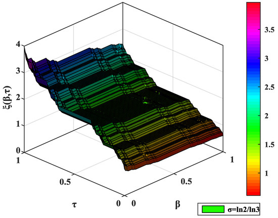
Figure 1. 3D plot of $\xi \left(\beta ,\tau \right)$ w.r.t. $\beta$ and $\tau$ in case of Example 1 for $\sigma =\ln 2/\ln 3$.

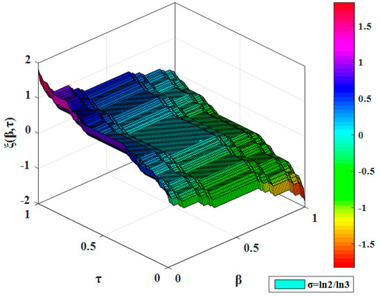
Figure 2. 3D plot of $\xi \left(\beta ,\tau \right)$ w.r.t. $\beta$ and $\tau$ in case of Example 2 for $\sigma =\ln 2/\ln 3$.

8. Conclusions

In this work, the solution of the LFLWR model of fractal vehicular traffic flow is examined through the implementation of LFNHAM and the LFNDM on the Cantor set. The novelty of the paper lies in the fact that the applied methods have never been used in the past for the considered LFLWR model. The efficiency of these methods is illustrated through two examples under distinct initial conditions and obtained results have been compared with solutions reported in past works. It is observed that the solutions for LFLWR models obtained through suggested methods are found in closed forms of fractal functions and are in good agreement with each other. Further, the LFNHAM gives a more general solution as compared to local fractional variational iteration method and local fractional natural homotopy perturbation method and assimilates their solutions as a special case. The 3D figures are illustrated for solutions of LFLWR model utilizing the MATLAB software. The surface graphics of the solution plotted on cantor set for the function $\xi \left(\beta ,\tau \right)$ possess fractal pattern. The computational results depict that the employed local fractional schemes are effective and beneficial to obtain the solution for the LFLWR model. However, there is also a limitation with these methods. These methods will be difficult to apply in the case of a non-evaluation of the LFNT. This study depicts that both of the methods are very reliable and can be utilized to solve different kinds of linear and nonlinear local fractional partial differential equations arising in fractal domain. As a future scope of the work, the applied methods can be extended to solve fractal form of physical and biological equations to explore new insights and reports in future.

References

- Peeta, S.; Ziliaskopoulos, A.K. Foundations of dynamic traffic assignment: The past, the present and the future. Netw. Spat. Econ. 2001, 1, 233–265. [Google Scholar] [CrossRef]
- Daganzo, C.F. A continuum theory of traffic dynamics for freeways with special lanes. Transp. Res. B Methodol. 1997, 31, 83–102. [Google Scholar] [CrossRef]
- Lighthill, M.J.; Whitham, G.B. On kinematic waves-II. A theory of traffic flow on long crowded roads. Proc. R. Soc. Lond. A Math. Phys. Eng. Sci. 1955, 229, 317–345. [Google Scholar]
- Richards, P.I. Shock waves on the highway. Oper. Res. 1956, 4, 42–51. [Google Scholar] [CrossRef]
- Zhang, H.M. New perspectives on continuum traffic flow models. Netw. Spat. Econ. 2001, 1, 9–33. [Google Scholar] [CrossRef]
- Li, T. L1 stability of conservation laws for a traffic flow model. Electron. J. Differ. Equ. 2001, 2001, 1–18. [Google Scholar]
- Gasser, I. On non-entropy solutions of scalar conservation laws for traffic flow. J. Appl. Math. Mech. 2003, 83, 137–143. [Google Scholar] [CrossRef]
- Aw, A.; Klar, A.; Materne, T.; Rascle, M. Derivation of continuum traffic flow models from microscopic follow-the-leader models. SIAM J. Appl. Math. 2002, 63, 259–278. [Google Scholar] [CrossRef]
- Bellomo, N.; Coscia, V. First order models and closure of the mass conservation equation in the mathematical theory of vehicular traffic flow. Comptes Rendus Mec. 2005, 333, 843–851. [Google Scholar] [CrossRef]
- Bellomo, N.; Delitala, M.; Coscia, V. On the mathematical theory of vehicular traffic flow—I: Fluid dynamic and kinetic modeling. Math. Models Methods Appl. Sci. 2002, 12, 1801–1843. [Google Scholar] [CrossRef]
- Ansorge, R. What does the entropy condition mean in traffic flow theory. Transp. Res. Part B 1990, 24, 133–143. [Google Scholar] [CrossRef]
- Towers, J.D. A splitting algorithm for LWR traffic models with flux discontinuities in the unknown. J. Comput. Phys. 2020, 421, 109722. [Google Scholar] [CrossRef]
- Bürger, R.; Chalons, C.; Ordoñez, R.; Villada, L.M. A multiclass Lighthill-Whitham-Richards traffic model with a discontinuous velocity function. Netw. Heterog. Media 2021, 16, 187–219. [Google Scholar] [CrossRef]
- Babakhani, A.; Gejji, V.D. On calculus of local fractional derivatives. J. Math. Anal. Appl. 2002, 270, 66–79. [Google Scholar] [CrossRef] [Green Version]
- Yang, X.J. Local Fractional Functional Analysis and Its Applications; Asian Academic: Hong Kong, China, 2011. [Google Scholar]
- Yang, X.J. Advanced Local Fractional Calculus and Its Applications; World Science: New York, NY, USA, 2012. [Google Scholar]
- Yang, X.J.; Srivastava, H.M.; Cattani, C. Local fractional homotopy perturbation method for solving fractional partial differential equations arising in mathematical physics. Rom. Rep. Phys. 2015, 67, 752–761. [Google Scholar]
- Zhang, Y.; Cattani, C.; Yang, X.J. Local fractional homotopy perturbation method for solving non-homogeneous heat conduction equations in fractal domains. Entropy 2015, 17, 6753–6764. [Google Scholar] [CrossRef] [Green Version]
- Yang, X.J.; Machado, J.A.T.; Hristov, J. Nonlinear dynamics for local fractional Burger’s equations arising in fractal flow. Nonlinear Dyn. 2016, 84, 3–7. [Google Scholar] [CrossRef] [Green Version]
- Ziane, D.; Baleanu, D.; Belghaba, K.; Cherif, M. Local fractional Sumudu decomposition method for linear partial differential equations with local fractional derivative. J. King Saud Univ. Sci. 2019, 31, 83–88. [Google Scholar] [CrossRef]
- Baleanu, D.; Jassim, H.K. A modification fractional homotopy perturbation method for solving Helmholtz and coupled Helmholtz equations on cantor sets. Fractal Fract. 2019, 3, 30. [Google Scholar] [CrossRef] [Green Version]
- Baleanu, D.; Jassim, H.K.; Al-Qurashi, M. Solving Helmholtz equation with local fractional derivative operators. Fractal Fract. 2019, 3, 43. [Google Scholar] [CrossRef] [Green Version]
- Singh, J.; Kumar, D.; Baleanu, D.; Rathore, S. On the local fractional wave equation in fractal strings. Math. Meth. Appl. Sci. 2019, 42, 1588–1595. [Google Scholar] [CrossRef]
- Liu, J.G.; Yang, X.J.; Feng, Y.Y.; Cui, P. A new perspective to study the third-order modified KDV equation on fractal set. Fractals 2020, 28, 2050110. [Google Scholar] [CrossRef]
- Li, X.X.; Tian, D.; He, C.H. A fractal modification of the surface coverage model for an electrochemical arsenic sensor. Electrochim. Acta 2019, 296, 491–493. [Google Scholar] [CrossRef]
- Dubey, V.P.; Singh, J.; Alshehri, A.M.; Dubey, S.; Kumar, D. A comparative analysis of two computational schemes for solving local fractional Laplace equations. Math. Meth. Appl. Sci. 2021, 44, 13540–13559. [Google Scholar] [CrossRef]
- Dubey, V.P.; Singh, J.; Alshehri, A.M.; Dubey, S.; Kumar, D. A hybrid computational method for local fractional dissipative and damped wave equations in fractal media. Waves Random Complex Media 2022, 1–23. [Google Scholar] [CrossRef]
- Dubey, V.P.; Singh, J.; Alshehri, A.M.; Dubey, S.; Kumar, D. An efficient analytical scheme with convergence analysis for computational study of local fractional Schrödinger equations. Math. Comput. Simul. 2022, 196, 296–318. [Google Scholar] [CrossRef]
- Dubey, V.P.; Singh, J.; Alshehri, A.M.; Dubey, S.; Kumar, D. Analysis of local fractional coupled Helmholtz and coupled Burgers’ equations in fractal media. AIMS Math. 2022, 7, 8080–8111. [Google Scholar] [CrossRef]
- Dubey, S.; Dubey, V.P.; Singh, J.; Alshehri, A.M.; Kumar, D. Computational study of a local fractional Tricomi equation occurring in fractal transonic flow. J. Comput. Nonlinear Dynam. 2022, 17, 081006. [Google Scholar] [CrossRef]
- Gao, W.; Baskonus, H.M. Deeper investigation of modified epidemiological computer virus propagation model containing the Caputo operator. Chaos Solitons Fractals 2022, 158, 112050. [Google Scholar] [CrossRef]
- Veeresha, P.; Ilhan, E.; Prakash, D.G.; Baskonus, H.M.; Gao, W. A new numerical investigation of fractional order susceptible-infected-recovered epidemic model of childhood disease. Alex. Eng. J. 2022, 61, 1747–1756. [Google Scholar] [CrossRef]
- Ciancio, A.; Yel, G.; Kumar, A.; Baskonus, H.M.; Ilhan, E. On the complex mixed dark-bright wave distributions to some conformable nonlinear integrable models. Fractals 2022, 30, 2240018. [Google Scholar] [CrossRef]
- Chen, Q.; Baskonus, H.M.; Gao, W.; Ilhan, E. Soliton theory and modulation instability analysis: The Ivancevic option pricing model in economy. Alex. Eng. J. 2022, 61, 7843–7851. [Google Scholar] [CrossRef]
- Sabir, Z.; Wahab, H.A.; Javeed, S.; Baskonus, H.M. An efficient stochastic numerical computing framework for the nonlinear higher order singular models. Fractal Fract. 2021, 5, 176. [Google Scholar] [CrossRef]
- Wang, L.F.; Yang, X.J.; Baleanu, D.; Cattani, C.; Zhao, Y. Fractal dynamical model of vehicular traffic flow within the local fractional conservation laws. Abstr. Appl. Anal. 2014, 2014, 1–5. [Google Scholar] [CrossRef]
- Yang, X.J.; Baleanu, D.; Machado, J.A.T. Systems of Navier-Stokes equations on Cantor sets. Math. Probl. Eng. 2013, 2013, 1–8. [Google Scholar] [CrossRef] [Green Version]
- Hao, Y.J.; Srivastava, H.M.; Jafari, H.; Yang, X.J. Helmholtz and diffusion equations associated with local fractional derivative operators involving the Cantorian and Cantor-type cylindrical coordinates. Adv. Math. Phys. 2013, 2013, 1–5. [Google Scholar] [CrossRef] [Green Version]
- Zhao, Y.; Baleanu, D.; Cattani, C.; Cheng, D.F.; Yang, X.J. Maxwell’s equations on Cantor sets: A local fractional approach. Adv. High Energy Phys. 2013, 2013, 1–6. [Google Scholar] [CrossRef] [Green Version]
- Yang, A.M.; Cattani, C.; Zhang, C.; Xie, G.N.; Yang, X.J. Local fractional Fourier series solutions for non-homogeneous heat equations arising in fractal heat flow with local fractional derivative. Adv. Mech. Eng. 2014, 2014, 1–5. [Google Scholar]
- Guo, Y.M.; Zhao, Y.; Zhou, Y.M.; Xiao, Z.B.; Yang, X.J. On the local fractional LWR model in fractal traffic flows in the entropy condition. Math. Meth. Appl. Sci. 2017, 40, 6127–6132. [Google Scholar] [CrossRef]
- Li, Y.; Wang, L.F.; Zeng, S.D.; Zhao, Y. Local fractional Laplace variational iteration method for fractal vehicular traffic flow. Adv. Theor. Math. Phys. 2014, 2014, 649318. [Google Scholar] [CrossRef]
- Singh, N.; Kumar, K.; Goswami, P.; Jafari, H. Analytical method to solve the local fractional vehicular traffic flow model. Math. Meth. Appl. Sci. 2022, 45, 3983–4001. [Google Scholar] [CrossRef]
- Jassim, H.K. On approximate methods for fractal vehicular traffic flow. TWMS J. App. Eng. Math. 2017, 7, 58–65. [Google Scholar]
- Kumar, D.; Tchier, F.; Singh, J.; Baleanu, D. An efficient computational technique for fractal vehicular traffic flow. Entropy 2018, 20, 259. [Google Scholar] [CrossRef] [PubMed] [Green Version]
- Zhao, D.; Singh, J.; Kumar, D.; Rathore, S.; Yang, X.J. An efficient computational technique for local fractional heat conduction equations in fractal media. J. Nonlinear Sci. Appl. 2017, 10, 1478–1486. [Google Scholar] [CrossRef] [Green Version]
- Singh, J.; Kumar, D.; Nieto, J.J. A reliable algorithm for local fractional Tricomi equation arising in fractal transonic flow. Entropy 2016, 18, 206. [Google Scholar] [CrossRef] [Green Version]
- Kumar, D.; Singh, J.; Baleanu, D. A hybrid computational approach for Klein-Gordon equations on Cantor sets. Nonlinear Dyn. 2017, 87, 511–517. [Google Scholar] [CrossRef]
- Jafari, H.; Jassim, H.K.; Moshokoa, S.P.; Ariyan, V.M.; Tchier, F. Reduced differential transform method for partial differential equations within local fractional derivative operators. Adv. Mech. Eng. 2016, 8, 1–6. [Google Scholar] [CrossRef] [Green Version]
- Keskin, Y.; Oturanc, G. Reduced differential transform method for partial differential equations. Int. J. Nonlinear Sci. Numer. Simul. 2009, 10, 741–750. [Google Scholar] [CrossRef]
- Ziane, D.; Bokhari, A.; Belgacem, R. Local fractional homotopy analysis method for solving coupled nonlinear systems of Burger’s equations. Int. J. Open Probl. Comput. Math. 2019, 12, 47–57. [Google Scholar]
- Maitama, S.; Zhao, W. Local fractional homotopy analysis method for solving nondifferentiable problems on Cantor sets. Adv. Differ. Equ. 2019, 2019, 1–22. [Google Scholar] [CrossRef] [Green Version]
- Baleanu, D.; Machado, J.A.T.; Cattani, C.; Baleanu, M.C.; Yang, X.J. Local fractional variational iteration and decomposition methods for wave equation on cantor sets within local fractional operators. Abstr. Appl. Anal. 2014, 2014, 1–6. [Google Scholar] [CrossRef]
- Yang, X.J.; Baleanu, D.; Zhong, W.P. Approximate solutions for diffusion equations on cantor space-time. Proc. Rom. Aca. Ser. A 2013, 14, 127–133. [Google Scholar]
- Yang, X.J.; Baleanu, D.; Lazarevic, M.P.; Cajic, M.S. Fractal boundary value problems for integral and differential equations fractional operators. Therm. Sci. 2015, 19, 959–966. [Google Scholar] [CrossRef]
- Maitama, S. Local fractional natural homotopy perturbation method for solving partial differential equations with local fractional derivative. Prog. Fract. Differ. Appl. 2018, 4, 219–228. [Google Scholar] [CrossRef]
- Jafari, H.; Jassim, H.K.; Al Qurashi, M.; Baleanu, D. On the existence and uniqueness of solutions for local fractional differential equations. Entropy 2016, 18, 420. [Google Scholar] [CrossRef] [Green Version]
- Khan, Z.H.; Khan, W.A. N-transform properties and applications. NUST J. Eng. Sci. 2008, 1, 127–133. [Google Scholar]
- Belgacem, F.B.M.; Silambarasan, R. Theory of the natural transform. Math. Eng. Sci. Aerosp. (MESA) J. 2012, 3, 99–124. [Google Scholar]
- Belgacem, F.B.M.; Silambarasan, R. Advances in the Natural Transform. AIP Conf. Proc. 2012, 1493, 106–110. [Google Scholar]
- Silambarasan, R.; Belgacem, F.B.M. Application of the Natural Transform to Maxwell’s Equations. In Proceedings of the Progress in Electromagnetics Research Symposium, Suzhou, China, 12–16 September 2011; pp. 899–902. [Google Scholar]
- Odibat, Z.; Bataineh, S.A. An adaptation of homotopy analysis method for reliable treatment of strongly nonlinear problems: Construction of homotopy polynomials. Math. Meth. Appl. Sci. 2014, 38, 991–1000. [Google Scholar] [CrossRef]
Publisher’s Note: MDPI stays neutral with regard to jurisdictional claims in published maps and institutional affiliations. |
© 2022 by the authors. Licensee MDPI, Basel, Switzerland. This article is an open access article distributed under the terms and conditions of the Creative Commons Attribution (CC BY) license (https://creativecommons.org/licenses/by/4.0/).