Abstract
The Pavement Condition Index (PCI) is a prevalent metric for assessing the condition of rigid pavements. The PCI calculation involves evaluating 19 types of damage. This study aims to analyze how different types of damage impact the PCI calculation and the impact of the performance of prediction models of PCI by reducing the number of evaluated damages. The Municipality of León, Gto., Mexico, provided a dataset of 5271 records. We evaluated five different decision-tree models to predict the PCI value. The Extra Trees model, which exhibited the best performance, was used to assess the feature importance of each type of damage, revealing their relative impacts on PCI predictions. To explore the potential for reducing the complexity of the PCI evaluation, we applied Sequential Forward Search and Brute Force Search techniques to analyze the performance of models with various feature combinations. Our findings indicate no significant statistical difference in terms of Mean Absolute Error (MAE) and the coefficient of determination (R2) between models trained with 13 features compared to those trained with all 17 features. For instance, a model using only eight damages achieved an MAE of 4.35 and an R2 of 0.89, comparable to the 3.56 MAE and 0.92 R2 obtained with a model using all 17 features. These results suggest that omitting some damages from the PCI calculation has a minimal impact on prediction accuracy but can substantially reduce the evaluation’s time and cost. In addition, knowing the most significant damages opens up the possibility of automating the evaluation of PCI using artificial intelligence.
1. Introduction
Evaluating the performance of rigid pavements in urban areas is crucial. This process informs the planning and prioritization of rehabilitation efforts, ensuring that the necessary works are scheduled efficiently. Such evaluations are also vital for coordinating construction activities and allocating the financial resources required for the successful execution of these projects. There are two types of pavement: flexible and rigid pavements []. The former corresponds to the bearing layer built with asphalt concrete, mainly observed in highways. In contrast, the latter is built with hydraulic concrete, which is used in urban areas. For several years, efforts have been made to determine indices that help explain the performance of pavements, among which the following stand out: Present Serviceability Rating (PSR) [], which has a subjective basis for its determination; the Present Serviceability Index (PSI) [,], which represents one of the first efforts to provide objectivity to pavement performance; and the International Roughness Index (IRI) [], which takes into account the effect of pavement irregularity on its performance. Those indices are commonly used in highways, on which, due to high speeds, the effect of irregularity in the longitudinal profile of the pavement is significant []. On the other hand, some methodologies are based on the evaluation of pavement damage but without obtaining an index that combines all the damage characteristics, as in the case of the Strategic Highway Research Program (SHRP) [] methodology. There is also work that has developed specific models based on studies carried out over several years, and which ultimately led to the implementation of software such as HDM4 [], promoted by the World Bank, which has its main application in roads, having options for optimizing conservation strategies with indicators such as the IRI. In contrast, the Pavement Condition Index (PCI) [] is recommended, especially in urban areas, where the speed of movement of vehicles is low compared to highways. It is based on the physical condition or flaws that the pavement presents [].
The PCI methodology proposed by the United States Corps of Engineers has been widely used []. It takes values between 0% and 100%, for pavements in poor condition and those in excellent condition, respectively []. In the case of rigid pavement, which is our interest in this work, the PCI is calculated from 19 different types of damage that commonly occur in this type of pavement, which include failures related to different types of cracking, deformations (faulting), and other surface defects such as wear or erosion [,]. The measurement of pavement deterioration and its modeling requires complex empirical models to capture it []. In this sense, machine learning has been applied in this task of pavement evaluation. The documents that propose machine learning in pavement evaluation use Neural Networks [,,,,], Support Vector Machines [], Levenberg–Marquardt, Bayesian Regularization, Scaling Conjugate Gradient [], Random Forests, Logistic Regression, and K-Neighbors [,]. While these documents demonstrate the potential of machine-learning models in predicting PCI, there exists a lack of sensitivity analyses to determine the importance of features (damages).
This research emphasizes identifying critical damages in calculating the PCI. The accurate assessment of these damages offers significant advantages. While qualified professionals typically conduct damage surveys, variations in evaluation and classification between different assessors are common, leading to discrepancies in damage quantification. Therefore, it is crucial to identify the damages that most significantly impact the PCI value, ensuring that these are assessed with particular precision. Furthermore, reducing the damage required for PCI calculation can minimize the time and cost associated with pavement evaluation. Finally, identifying the most impactful damages could facilitate the development of automated PCI evaluation technologies, such as the methodologies that used computer vision proposed in [,,,,,]. Some of the previous work done in the sensitivity analysis of damages or for selecting some features for pavement evaluation are described as follows. Suh et al. analyzed Korean highways with asphalt pavement; a sensitivity analysis was carried out to detect the variables that had a significant effect (IRI, rut depth, and cracking) on pavement condition, which later allowed the development of a model of a single index applicable to the entire road network analyzed []. Kwak et al. developed a sensitivity analysis to detect the variables that most influence the PCI in rigid pavements. They used data from airports and used nonlinear regression techniques. They do not consider the variables of the failures or damages that are used directly to calculate the PCI. However, they focused on verifying the impact of other pavement attributes, such as the age of the concrete slab, accumulated traffic, weather conditions, thickness of the slab, modulus of reaction, and maintenance time. From this study, it was observed that the variable that has the most impact on the PCI is the age of the concrete slab, which shows the highest correlation []. Documents show the possibility of relating PCI in rigid pavements directly with the damage variables evaluated in the field [,]. They obtained expressions that correlate those variables with the PCI and other indicators. Other studies also show a greater incidence of certain variables on the PCI [,,], which leads us to consider the possibility of reducing the number of variables involved in the calculation. However, those documents do not justify how variables are selected. Studies carried out on asphalt pavements show a strong correlation between the PCI and the most frequent damages, such as longitudinal and transverse cracks, ruts, and potholes [,]. These studies have shown little effect of not considering some variables in the analysis. However, the selection process of the variables is not justified either. The literature review reveals a significant gap in the analysis of critical damages as defined by the original Pavement Condition Index (PCI) calculation method. Specifically, there is a need for a deeper understanding of how each type of damage influences the PCI calculation and how the inclusion or exclusion of certain features impacts the accuracy and effectiveness of PCI evaluation.
Summing up, this study aims to perform a sensitivity analysis to identify the most significant damages or features for calculating the Pavement Condition Index (PCI). This will enable us to identify the critical damages necessary for accurately assessing pavement conditions and those that may be less important and can potentially be omitted. For the analysis, we use a real database that consists of 5271 samples or segments of pavement, obtained in an approximate length of 369 km, located in León, Gto. México. Each pavement segment consists of 20 slabs on average, with typical dimensions of 3.50 × 3.50 m each. We are considering only slabs and granular bases (non-chemically stabilized bases) without continuous reinforcing and prestressing. It is important to mention that the dataset is available online in []. We analyze each variable using correlation and feature importance, calculated through tree-based prediction models, including Decision Trees, Random Forest, AdaBoost, Extra Trees, and Gradient Boosting. We employ methods like Sequential Forward Search and Brute Force Search to assess model performance across different feature combinations. Our findings are presented in terms of the coefficient of determination and mean absolute error, highlighting the impact of each damage type within the models.
The rest of the paper is organized as follows. Section 2 describes the methodology for the PCI evaluation. The methodology, where the data and the applied techniques are described, is presented in Section 3. The experiments and results can be seen in Section 4. Section 5 presents the discussion. Finally, the conclusion of this paper is presented in Section 6.
2. Pavement Condition Index (PCI)
The Pavement Condition Index (PCI) [] is the most comprehensive methodology for objectively evaluating and rating flexible and rigid pavements. It is easy to implement and does not require specialized tools beyond those that constitute the system. The PCI calculation is based on the results of a visual inventory of the pavement condition, which establishes the class, severity, and quantity of each damage. Figure 1 shows some of the most frequently occurring damages in concrete pavements. Formulating an index considering all three factors has been problematic due to many possible conditions. To overcome this difficulty, Deduct Values were introduced as an archetypal weighting factor to indicate the degree of impairment of each damage class combination. The PCI was developed to assess the pavement’s structural integrity and the surface’s operational condition. The damage information obtained as part of the inventory provides a clear insight into the causes of the damage and its relationship to loads or climate.
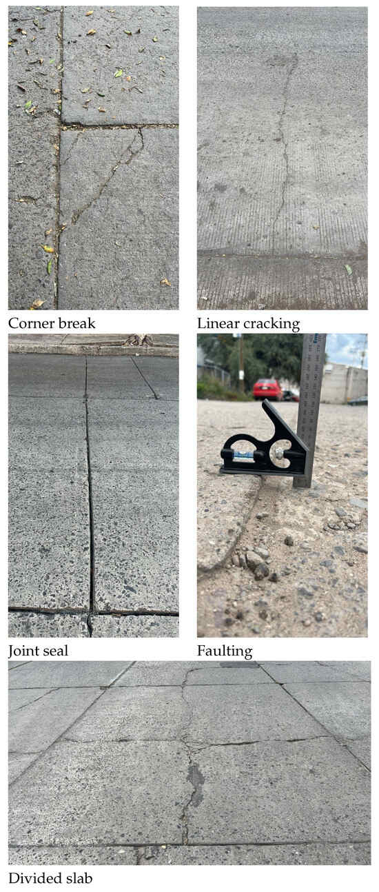
Figure 1.
Some of the most frequent damages in concrete pavement.
The PCI is a numerical index that varies from zero (0) for failed or poor pavement to one hundred (100) for pavement in perfect condition. Table 1 presents the PCI ranges with the corresponding qualitative description of the pavement condition.

Table 1.
PCI evaluation ranges.
Calculating the Pavement Condition Index (PCI) involves three primary phases. First is the selection of sampling units for inspection. At the network level, sampling units are chosen based on statistical procedures to meet a specified confidence level. In contrast, all identified units must be inspected at the project level. The second phase consists of the pavement condition assessment; this procedure varies depending on the pavement surface type. It is essential to adhere strictly to the damage definitions provided in the PCI manual during this phase. The final phase is the calculation of PCI for sampling units. After the field inspection, the collected damage data is used to calculate the PCI. This calculation can be performed manually or with the help of software, depending on the deduct values assigned to each type of damage, considering its extent and severity.
Broadly speaking, the description of the PCI calculation is as follows (more details in []):
- Count he Damage Occurrences: Identify and count the slabs affected by each combination of damage type and severity level within the sampling unit.
- Calculate Damage Density: Divide the number of affected slabs by the total number of slabs in the unit, expressing the result as a percentage (%). This percentage represents the damage density for each type of damage at its respective severity level.
- Determine Deduct Values: Use the appropriate Deduct Value curve from the PCI manual to find the deduct value for each damage type and severity level combination. Figure 2 shows an example of a graph that obtains the deduct value for a particular damage (linear cracking). The deduct value will be obtained from the density and severity of the damage in question.
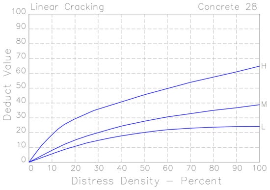 Figure 2. Example of a graph for obtaining the deduct values. Adapted from [].
 - Calculate the Maximum Allowable Deduct Value: Sum the deduct values to determine the Total Deduct Value (TDV) for the unit.
- Correct the Deduct Value (CDV): Use the PCI manual to calculate the CDV, which accounts for the total deduct values in a way that prevents overestimation of the pavement’s deterioration (see Figure 3).
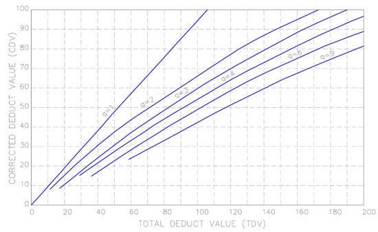 Figure 3. Example of a graph for obtaining the total deduct value. The value of q is defined as the number of deducts values greater than 2 points. Adapted from [].
 - Compute the PCI: Finally, subtract the maximum CDV from 100 to obtain the PCI for the unit.
PCI is commonly chosen as an indicator for pavement assessment due to several advantages. First, its procedure presents a complete methodology for implementing a pavement management system at the network or project level, setting out precise guidelines for doing so. In the assessment of damages, the practicality of a single indicator in PCI implies an accessible interpretation, especially when geographic information systems are used to identify sections with different PCI values or their condition quickly, making its application straightforward.
This methodology has been used in the Municipality of León, Guanajuato, Mexico, for several years. The data collected can serve as a reference for applying the methodology and its benefits to other areas with similar characteristics.
3. Materials and Methods
This section presents the data and the models used in the sensitivity analysis of the damages used in the PCI evaluation. First, we present the data proportionated by the Dirección General de Obra Pública, of León City in Guanajuato, México, and some figures to show the distribution and correlation of the data. Finally, we describe the regression models based on trees that are used in the analysis: Decision Trees, Random Forest, AdaBoost, Extra Trees, and Gradient Boosting.
3.1. Data
The Dirección General de Obra Pública, which is a department of the Government in León City in Guanajuato, México, in charge of public work, proportionated the dataset used in this research. This data is used to analyze the maintenance and operation of roads. It comprises 5271 evaluated segments, approximately 369 km, corresponding to Portland Cement concrete pavements for principal and secondary roads. Each pavement segment consists of 20 slabs on average, with typical dimensions of 3.50 × 3.50 m each. Figure 4 shows the location of the area under study and a close-up of the city of León, Guanajuato. All pavements are simple concrete slabs; that is, they do not consider continuous reinforcement or prestress, except for the dowel bars placed in the transverse joints and the corrugated tie bars located in the longitudinal joints. Each segment or sampling unit consists of slabs, considering each slab is less than 4.20 m long, presenting a maximum length/width ratio of 1.25 m. This work studies pavement structures consisting of a simple concrete slab, without considering reinforcing steel or continuous prestress, except for the corrugated tie bars and dowel bars. These slabs are built on a granular base (not chemically stabilized). The different types of damage were quantified, and the PCI was calculated using the methodology of the United States Army Corps of Engineers []. It is worth mentioning that the damage corresponding to freezing was not considered since, due to the climate characteristics in León, Gto., México, temperatures do not drop to the point of having this effect. Failures due to railroad crossings were not considered either because the analyzed segments did not have this type of crossing and were concessioned to private companies. Therefore, the data used only 17 variables, as seen in Table 2. Table 3 shows an example of some dataset rows. The first 17 columns are the damages, and the last corresponds to the PCI value. The dataset contains 5271 rows, each one representing a segment. It is important to mention that the dataset is available online in [].
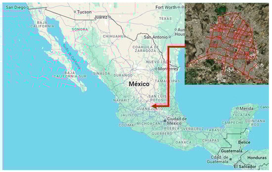
Figure 4.
Map illustrating the location of the study area, with the evaluated segments highlighted in red.
Table 2.
Damage nomenclature.
Table 3.
Example of some rows of the dataset. All values represent percentages.
The nomenclature shown in Table 2 will be used throughout this article. The description of each type of damage is presented below:
- Blowup – Buckling: occurs in warm weather, usually in a crack or transverse joint that is not wide enough to allow expansion of the slab. Insufficient width is usually due to the infiltration of incompressible materials into the joint space. When expansion cannot dissipate sufficient pressure, upward movement of the slab edges (buckling) or fragmentation will occur near the joint.
- Corner break: A corner break is a crack that intersects the joints of a slab at a distance less than or equal to half the length of the slab on both sides, measured from the corner. Generally, the repetition of loads combined with the loss of support and warping stresses cause corner cracks.
- Divided slab: The slab is divided by cracks into four or more parts due to overloading or inadequate support. If all parts or cracks are contained in a corner crack, the damage is classified as a severe corner crack.
- Faulting: The difference in level across the joint. Some common causes that originate from it are those related to settlement, erosion, or warping of the slabs.
- Joint seal damage: Any condition that allows soil or rock to accumulate in the joints or that allows significant water infiltration. Accumulating incompressible material prevents the slab from expanding and can result in splintering, lifting, or spalling of the joint edges. A suitable filling material prevents this from happening.
- Lane/Shoulder drop-off: The difference between the settlement or erosion of the shoulder and the edge of the pavement. The difference in levels can constitute a security threat. It can also be caused by increased water infiltration.
- Linear cracking: These cracks divide the slab into two or three pieces and are usually caused by repeated traffic loads and warping due to thermal or humidity gradients.
- Patching large: An area where the original pavement has been removed and replaced by new material (greater than 0.45 m2). A utility excavation is a pothole that has replaced the original pavement to allow for the installation or maintenance of underground facilities.
- Patching small: An area where the original pavement has been removed and replaced by a filling material 0.45 m2).
- Polished aggregate: This damage is caused by repeated applications of traffic loads. When the aggregates on the surface become soft to the touch, the adhesion with the tires is significantly reduced. When the portion of the aggregate that extends over the surface is small, the pavement texture does not significantly contribute to reducing vehicle speed.
- Popouts: A small part of the pavement that detaches from the surface of the same. It may be due to soft particles worn by traffic. They vary in size, with diameters between 25.0 mm and 102.0 mm, and thicknesses from 13.0 mm to 51.0 mm.
- Pumping: The expulsion of material from the foundation of the slab through the joints or cracks. The deflection of the slab is caused by the loads. When a load passes over the joint between the slabs, the water is first forced under the front slab and then backward under the rear slab. This action causes erosion and eventually removes soil particles, leading to progressive pavement support loss.
- Punchout: This damage is a localized area of the slab that is broken into pieces. This damage is caused by repeated heavy loads, inadequate slab thickness, loss of foundation support, or a localized deficiency of concrete construction.
- Scaling/Map cracking/crazing: Refers to a network of superficial hairline or capillary cracks extending only to the concrete surface’s upper part. Cracks tend to intersect at 120-degree angles. Generally, this damage occurs due to excessive handling in the finish. It can cause flaking, which is the cracking of the slab’s surface to an approximate depth of 6.0 mm to 13.0 mm. Incorrect construction and poor-quality aggregates can also cause it.
- Shrinkage cracks: These are hairline cracks, usually short in length, and do not extend along the entire length of the slab. They are formed during the setting and curing of concrete.
- Spalling corner: The breaking of the slab approximately 0.6 m from the corner. A corner spall differs from a corner crack in that the spall usually dips down to intersect the joint. In contrast, the crack extends vertically through the slab corner.
- Spalling joint: Breaks the slab’s edges approximately 0.60 m from the joint. It does not extend vertically through the slab but rather intersects the joint at an angle.
Figure 5 shows boxplots for each type of damage to note the distribution of the percentages for each type and the distribution of the PCI. A boxplot provides a summary of a dataset’s distribution. The central box represents the Interquartile Range (IQR), encompassing the middle 50% of the data, with the line inside the box indicating the median. The ’whiskers’ extend from the box to the smallest and largest values within 1.5 times the IQR from the quartiles. Data points outside this range are plotted as outliers. From Figure 5, it can be observed that some features have more dispersion than others. For example, Jseal and Scal are the features with the biggest dispersion. In contrast, Blowup, Faulti, and LaneDF have less dispersion.
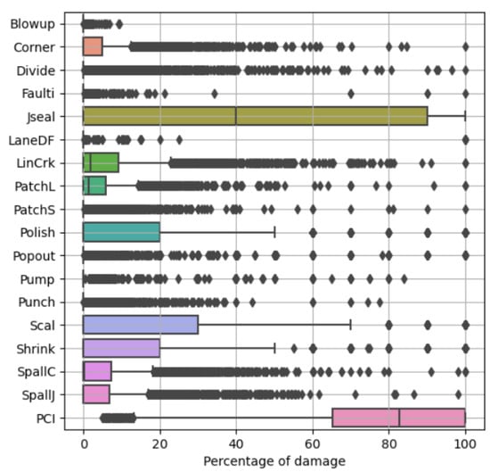
Figure 5.
Distribution of type of damages and PCI values.
Figure 6 shows the PCI distribution based on its magnitude, as described in Table 1. It can be noted that most of the data is in the good, satisfactory, or fair range. The average and standard deviation are 77.91% and 22.39%, respectively.
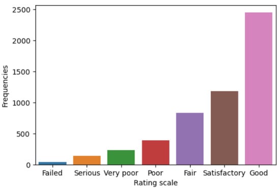
Figure 6.
Distribution of PCI values.
Figure 7 shows the Pearson correlation coefficient between the type of damage and the PCI. The variables that have strong linear dependencies with PCI, the ones with absolute correlation values close to 1, are LinCrk, Jseal, SpallC, SpallJ, Divide, and Corner. For example, once the loss of sealing in joints (Jseal) appears, it is typical for spalling to appear in the short term in joints (SpallJ) and corners (SpallC). This is due to the inclusion of incompressible material in the unsealed joints, which prevents the free movement of expansion and contraction of the slabs, generating stresses that break the concrete in those areas. On the other hand, cracking (LinCrk) is usually related to overstressing that the slabs cannot resist, generating longitudinal, transverse, and corner cracks (Corner), and in a more advanced degree of deterioration, divided slabs (Divide); this may be due to an inadequate thickness of the slab or to poor quality of the foundation ground.
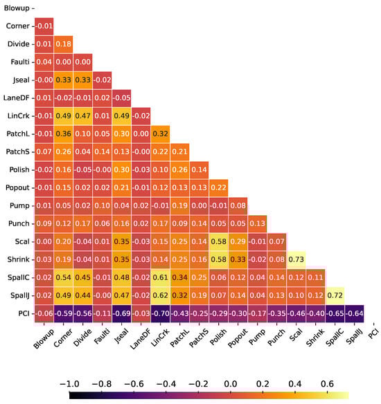
Figure 7.
Pearson correlation between types of damage and PCI.
3.2. PCI Prediction Based on Trees Regression Models
As we explained previously, the PCI is a numerical value used to represent the overall condition of a pavement. It is typically determined based on various observed damages (see Table 2). In the context of our research, we aim to predict the PCI by leveraging machine-learning techniques. Regression models, a subgroup of machine-learning algorithms, aim to find relationships between input and output numeric variables to make predictions. In this case, the input variables are the 17 damages and the output variable corresponds to the PCI value. Based on the example in Table 3, the input variables are the first 17 columns and the output variable is the last.
Therefore, regression is about fitting a mathematical model that relates input variables to an output variable, which tries to reduce an error. Mathematically, we can express the regression as follows: given a set of input–output data pairs, , where and , the learning process can be defined as a problem where a function, f, must be found that minimizes , where L is a function that measures the difference or error between and y. The ideal scenario would be . Sometimes, the function can be expressed as . In this case, each pair of represents the values of pavement damages, , and their corresponding PCI value, y, for each one of the slabs. The objective is to reduce the difference of the real value of the PCI, or y, with the prediction of the model using the values of the damages.
In this research, we decided to use regression models based on trees because they are non-parametric methodologies, meaning they do not assume a specific data distribution. In addition, they allow us to calculate the feature importance that represents how significant each variable is for the regression model. Decision trees [] are algorithms whose models are based on “if” type comparisons; with this process, the prediction of an output variable, y, is related to other input variables, . The decision-tree algorithm is one of the most widely used machine-learning algorithms for solving classification and regression problems. As the name suggests, the algorithm uses a tree data structure to predict the target value (see Figure 8).
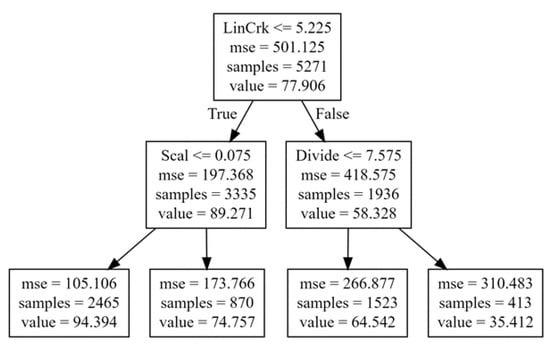
Figure 8.
An example of a small decision tree.
The tree-building process begins with the root node. The algorithm selects the variable that best splits the data and creates a node for that variable. The dataset is then further split based on the answer to the current node’s question, thus creating additional tree branches. The objective of splitting the data is to reduce the impurity of the data in the node; in this case, the impurity is calculated with the mean squared error. Processing continues recursively until a stopping condition is reached, such as when all leaf nodes have null impurity or a maximum number of levels is reached. Once the tree has been built, it is used to predict the new data target. The path is followed from the root node to a leaf in the tree, using the values of the input variables to answer the questions at each node and determine the path to follow. Finally, a leaf in the tree is reached that contains a prediction for the target variable. As shown in the example of Figure 8, the root node begins to evaluate the LinCrk damage. If its value is less than 5.225, it takes the path to the left. Otherwise, the process continues to the right. Following the corresponding path, the leaf node contains the value of the corresponding prediction.
As we mentioned previously, models based on decision trees have the advantage of allowing an analysis of feature importance, representing the proportionality of the impurity reduction of all nodes related to the variable in question []. The Impurity Reduction (IR) at each node j can be determined with Equation (1), where and represent the branch nodes of node j, I represents the impurity of each node, and the weights, w, are the proportion of the samples in the nodes and are calculated as the number of samples in the node divided by the total number of samples.
Once the impurity reduction at all nodes is known, the feature importance, , of the variable k is calculated using Equation (2), where represents the set of all nodes split using the variable k, and N represents all nodes in the decision tree.
Random Forest [] is a supervised-learning algorithm that uses an ensemble combining several decision trees. The ensemble-learning method is a technique that combines predictions from multiple models to make a more accurate prediction than a single one. The training process of trees is done independently of each other in parallel, without interaction between them. Each tree in the forest is different because they are trained with a random subset of samples and features from the original dataset. The prediction of the forest is calculated as the mean of the trees’ predictions. Figure 9 shows an example of how the prediction is made with a Random Forest composed of three trees. Another algorithm, called Extra Trees [], is similar to Random Forest but also considers randomness in the selection of the cutoff value (threshold) to divide each node. Instead of choosing the threshold that best divides each feature, a random cutoff value is generated for each proposed feature. Another difference with Random Forest is that the samples with which each tree is trained are chosen without replacement.
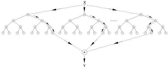
Figure 9.
An example of the prediction with a Random Forest.
Gradient Boosting [] is a prediction model composed of several decision trees trained sequentially so that each new tree tries to improve the errors of the previous ones. The prediction of a new observation is obtained by adding the predictions of all the previous individual trees that make up the model (see Figure 10). The process consists of building a tree with a single root node. Once this is done, the next step is to build a new tree from the errors of the previous tree, then a new tree is built again with the previous errors, and so on until the maximum number of trees is reached or until the new trees do not improve the fit. The final model to make the prediction combines all the trees. Ada Boost [] is also a supervised prediction model that creates several simple predictors in sequence so that the second fits what the first did not fit well, that the third fits better, what the second could not, and so on. It is similar to Gradient Boosting; the difference is that AdaBoost increases the weight or weights of previously misclassified observations, while Gradient Boosting identifies difficult observations using the residuals calculated in previous iterations.
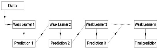
Figure 10.
Schematic process of Gradient Boosting; each weak learner is a decision tree.
4. Experiments and Results
To determine the significance of various damages in predicting the Pavement Condition Index (PCI), we performed a sensitivity analysis using the data and models described in Section 3. The models employed include Decision Trees, Random Forest, Extra Trees, Gradient Boosting, and Ada Boost. We designed three key experiments:
- Model performance analysis: We analyzed the performance of different regression models (Decision Trees, Random Forest, Extra Trees, Gradient Boosting, and Ada Boost) using all 17 available features. We computed the feature importance for each type of damage based on the model that showed the best performance. More details can be found in Section 4.4.
- Sequential feature inclusion: We performed a sensitivity analysis using the model selected from the first experiment. The main goal is to explore how the performance of prediction models would be affected if we changed the number of damages in the PCI calculation. This involved training the model initially with the most significant single feature, then incrementally adding features in order of importance, with a Sequential Forward Search []. This process was repeated until 17 models were developed, each incorporating an increasing number of features. This method allowed us to observe the impact of each additional variable on model performance. More details can be found in Section 4.5.
- Brute force feature analysis: Similar to the second experiment, this analysis utilized a Brute Force Search to evaluate the performance across all possible feature subsets; in other words, all the possible combinations of using or not using each feature. With 17 features, it represents a computationally intensive process. This approach considers potential redundancy among features, providing a comprehensive view of feature interactions and dependencies. More details can be found in Section 4.6.
All experiments were conducted using the Python programming language, supported by libraries such as Scikit-learn [], Pandas [], Matplotlib [], and NumPy []. Additionally, some of the graphics were generated using RStudio [].
4.1. Performance Metrics
This research evaluates the significance of each feature in predicting the Pavement Condition Index (PCI). To assess the performance of our proposed regression models, we employ two key metrics:
- Coefficient of determination (R2). This quantifies the quality of predictions relative to the variance in the output variable. A value of 1 indicates perfect model performance, while 0 suggests that the model performs no better than random guessing based on the output variable’s distribution. A negative R2 indicates that the model performs worse than random guesses.Mathematically, R2 is expressed according to Equation (3), where y represents the actual value of the output variable and represents the prediction value obtained from the model.
- Mean Absolute Error (MAE): This measures the average magnitude of errors in a set of predictions without considering their direction. It is the mean absolute difference between the actual values, y, and the predictions, . It is particularly useful as it provides an error metric in the same units as the data. Mathematically, MAE is expressed according to Equation (4), where n is the number of samples.
Together, R2 and MAE provide a comprehensive view of model performance. R2 assesses the model’s ability to capture the variance in the data, while MAE offers a straightforward, interpretable measure of average error magnitude.
4.2. Statistical Tests
The Friedman test is used to determine if there are statistically significant differences among multiple populations. It involves pairwise comparisons of the rankings assigned to these populations. If the Friedman test indicates significant differences, the Nemenyi post-hoc test is then applied to identify which specific populations differ significantly from each other. The analysis using the Nemenyi test relies on two key parameters: the Critical Difference (CD) and the average ranks of the populations derived from pairwise comparisons across all datasets. Demvsar [] introduces the Critical Difference (CD) plot to compare classifiers or treatments across multiple datasets. In a CD plot, the average ranks of treatments are displayed on the horizontal axis. Each treatment is represented by a bar, arranged according to their average ranks. Horizontal lines connect treatments that are not significantly different from each other based on the calculated critical difference. The CD is derived from the rank distribution and depends on the number of treatments and the desired significance level. If the distance between the average ranks of the two treatments exceeds the CD, it indicates a statistically significant difference between them.
In this paper, we evaluate the Friedman test at a significance level of 0.01, followed by the post-hoc Nemenyi test at a significance level of 0.05. We utilized the scmamp library [] to conduct the necessary statistical tests for our analysis.
4.3. Validation Strategies
To analyze and validate the performance of our prediction models, we employ two distinct strategies:
- Cross-Validation: Cross-validation was used for the first two experiments. It divides the dataset into k folds (in this case, 50), in which, in each iteration, 49 folds serve as the training set and one fold as the testing set. In this scenario, the model is trained and validated 50 times, changing the testing set each time. In total, we have 5271 samples, which in each iteration are divided into 5165 for training and 106 for tests. Using this validation strategy, all the samples are used for training and testing at some point.
- Train–Test Split: In the third and most resource-intensive experiment, we randomly divide the dataset into a training set (70%) and a testing set (30%). The models are fitted using the training data, and predictions and performance metrics are calculated using the testing data. This straightforward approach allows us to evaluate how well the models perform on unseen data.
These validation strategies are crucial for assessing the models’ abilities to generalize to new data and for ensuring that our findings are not merely reflective of a particular subset of data. Cross-validation, in particular, helps mitigate overfitting and provides a more accurate measure of model performance across various subsets of the dataset.
4.4. Experiment 1: Analysis of the Prediction with All Types of Damage
In the first experiment, we used the original 17 features to create and compare five models based on decision trees: Decision Trees, Random Forest, Extra Trees, Gradient Boosting, and Ada Boost. We use the sklearn implementation [] with the default parameters. To validate the models’ performance, we use cross-validation with 50 folds.
The values obtained from R2 and MAE are shown in Figure 11. Table 4 shows each model’s mean R2 and MAE values. It can be observed that the Extra Trees, Gradient Boosting, and Random Forest obtained good results—all of them with an R2 value higher than 0.9 on average. Regarding the analysis of MAE, it can be observed that the Extra Trees algorithm presents the lowest MAE values compared to the other methods.
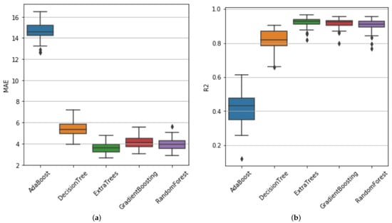
Figure 11.
Performance of the different tree models based on MAE (a) and R2 (b).
Table 4.
Mean values of R2 and MAE. The best result is shown in bold.
The Friedman test evaluates the null hypothesis of equal ranks for model performance. The chi-squared statistics obtained for this test were 186.99 and 172.21 for the MAE and R2 measures, respectively. Both chi-squared statistics rejected the null hypothesis, with p-values below 0.001. Therefore, we can conclude that certain models’ performances based on features statistically outperforms others. Regarding this rejection, the post-hoc Nemenyi test is applied. The critical difference, calculated at 0.8690, is depicted in the significance diagrams, as shown in Figure 12. Based on R2, we can observe no significant differences in the average rankings between Extra Trees and Gradient Boosting, with Extra Trees being the top-ranked model and Ada Boost the worst. Based on MAE, Extra Trees is the top-ranked model, with Ada Boost performing the worst. Extra Trees demonstrates statistically significant differences in ranking compared to all other models.
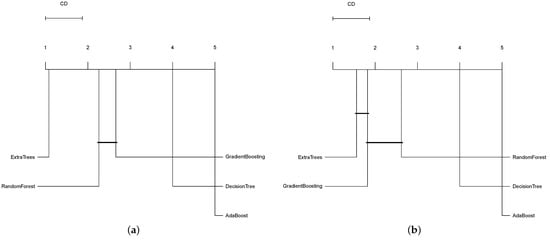
Figure 12.
CD plot of the Nemenyi statistical test comparing the different tree models based on MAE (a) and R2 (b). Groups of algorithms that are not significantly different are connected.
Once Extra Trees obtained the best rank in the models comparison, we calculated the feature importance using Extra Trees to find the most significant variables for predicting the PCI. Figure 13 presents the feature importance of each variable calculated using the values obtained from the 50 executions. In addition, Table 5 shows the average of the feature importance. It can be seen that there are variables that contribute significantly to the prediction model, such as Jseal, LinCrk, and Divide, while other features almost do not contribute, such as Blowup and LaneDF. It is important to remember that the feature importance value is defined in a range of 0 and 1, the lowest and highest, respectively. Figure 5 shows the dataset’s frequency of damages. We can observe that some of the features whose feature importance is high are those whose values in the dataset are high, for example, Jseal and LinCrk. However, we have the case of the feature Divide, whose feature importance is high and whose values in the dataset are small (see Figure 5).
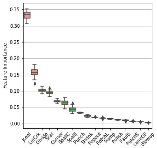
Figure 13.
Feature importances calculated with Extra Trees.
Table 5.
Average feature importance of damages.
Comparing the results of feature importance (Table 5) with the Pearson correlation coefficient between the PCI value and the features (see Figure 7), we can observe that features that have high feature importance also have a high linear correlation with the PCI, as in the case of Jseal, LinCrk, Divide, Scal, Corner, SpallC, and SpallJ. On one hand, the feature importance is a metric that shows how significant a feature is for the regression model. On the other hand, the absolute Pearson correlation coefficient measures the linear dependency between the variable and the PCI. In both cases, greater values, close to 1, indicate that the feature is important to the model, or it has a high dependency on the PCI.
The most important variable in this analysis was the joint seal damage, which can be caused by a deficiency in the placement or the quality of the material used. Once the sealing has been lost, and if it is not attended to and corrected, pavement deterioration begins, giving rise to the possibility of water entering through the joints, which will begin to generate a pumping process. The loss of support of the paving slab follows. This causes longitudinal, transverse, and corner cracking or, in a more advanced stage, divided slabs.
Certain damages, such as spall in joints and corners, are also usually the consequence of a loss of sealing in the joints, which allows the inclusion of incompressible materials that prevent the free movement of contraction and expansion of the slabs derived from thermal effects, generating breakage surface of the slab in these areas. Other damages, such as punchout cracking, usually appear after the mentioned damages, mainly when the foundation soil has significantly lost its resistance capacity or, in other cases, when the thickness of the slab is not designed correctly. In these cases, the slab becomes incapable of resisting vehicular loads.
Some damages tend to be more related to deficient construction processes, such as excessive surface manipulation when finishing and texturing the slabs, as in the case of surface cracking. Shrinkage cracking could be caused by late curing of the concrete or poor concrete mix design, especially where high water/cement ratios are present or by excess cement paste.
Although the pumping damage turned out to be number twelve according to the determination of the important variables, it should be noted that, in the case of concrete slabs, whose failure turns out to be brittle, it is not required to have a manifestation that is too severe so that a slight loss of support causes the cracking of the slabs, which is why said damage does not appear in the first places. The evaluators may not have adequately detected it due to the frequent sweeping of the pavement surface in urban areas, preventing the possibility of visualizing the accumulation of fine material on the surface.
4.5. Experiment 2: Sensitivity Analysis by a Sequential Forward Search
The second experiment performed a sensitivity analysis following a Sequential Forward Search []. The first model was trained with one variable, the most important one from the feature importance analysis presented in Experiment 1. The second model was trained with the two most important variables. The third model was fitted with the three most important features, and so on, until a model has been trained using all the variables. We used the Extra Trees model because it had the best results in Experiment 1. In total, 17 models were trained with the Extra Trees regressor algorithm. Cross-validation (k = 50) was used to validate each model to calculate the R2 and MAE metrics.
Figure 14 shows the R2 and MAE values obtained for each trained model. Table 6 shows the average performance values of R2 and MAE of these models. As more variables are included in the analysis, the MAE decreases, and the value of R2 increases, this effect being less significant as the number of variables increases.
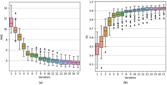
Figure 14.
Performance of the models trained with the subsets of variables found using Sequential Forward Search based on MAE (a) and R2 (b).
Table 6.
Performance of the models fitted with the subset of variables found in Sequential Forward Search (SFS) vs. Brute Force Search (BFS). Bold numbers represent the best result between SFS and BFS.
The Friedman test evaluates the null hypothesis of equal ranks for model performance fitted with the subsets of features found in Sequential Forward Search. The chi-squared statistics obtained for this test were 760.37 and 715.71 for the MAE and R2 measures, respectively. Both chi-squared statistics rejected the null hypothesis with p-values below 0.001. Therefore, certain models’ performances statistically outperform others. Regarding this rejection, the post-hoc Nemenyi test is applied. The critical difference, calculated at 3.5038, is depicted in the significance diagrams, as shown in Figure 15. It shows no significant differences in the average rankings of MAE between the model performance of the ones fitted with 13, 14, 15, 16, and 17 features because they belong to the same group. On the other hand, Figure 15 illustrates that models fitted with 12, 13, 14, 15, 16, and 17 variables have no significant differences based on R2. We can conclude from both statistical tests that we have not found significant differences between the models fitted with 13, 14, 15, 16, and 17 features of the subsets found with Sequential Forward Search.
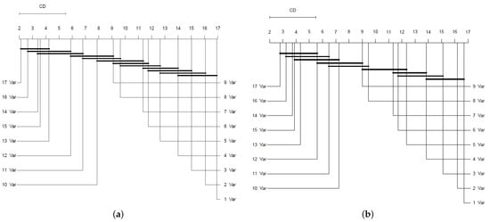
Figure 15.
CD plot of the Nemenyi statistical test comparing the models trained with subsets of variables found using Sequential Forward Search based on MAE (a) and R2 (b). Groups of algorithms that are not significantly different are connected.
From the above, the reader could consider more or fewer variables depending on the situation. One could evaluate only the first eight variables, mainly related to cracking and joint deficiencies, which are relatively easy to classify and measure in the field. If this were the case, an average MAE value of approximately 4.43% would be accepted, which, in principle, seems reasonable if other errors related to the evaluator’s expertise or other impediments that frequently result in the zones are considered. For example, parked vehicles that make it impossible to adequately observe and measure the pavement’s damage or the traffic intensity on certain roads significantly complicate measuring and classifying the damage. The average MAE value obtained with the prediction model using the 17 variables is only 3.56%. In that case, it can be seen that the error when using eight variables increases by only 0.87%. Similarly, if only the first five most important variables are considered, the increase in the MAE compared to the model that uses 17 variables is only 1.8%.
4.6. Experiment 3: Sensitivity Analysis by a Brute Force Search
The previous experiment consisted of a sensitivity analysis using Sequential Forward Search, which consisted of adding the feature with the more significant value according to the feature’s importance one by one. This analysis is interesting; however, it does not consider if features are redundant among them. For example, in Figure 7 it can be observed that several features are highly correlated among them. This experiment consists of a Brute Force Search analyzing the performance of all possible combinations of taking or not each feature.
In this experiment, we aim to analyze the performance of all the possible subsets of features. Some examples of subsets of features can be A = {Jseal}, B = {Divide, Scal}, C = {Divide, Jseal}, or D = {Scal, Divide, LinCrk, Corner, Punch, Jseal, Poput, SpallC, Pump, PatchL, Polish, Shrink, Blowup, Faulti, LaneDF, SpallJ, PatchS}. We can see that D is composed of all 17 features, contrary to A, which is composed only of the Jseal feature. C and D have two features, but they are different subsets. Each subset can be represented as a binary vector with 17 entries, where each entry represents the fact of taking or not a specific feature. Following the feature enumeration of Table 2, the subset B could be represented as the vector , which corresponds to selecting only the 3rd and 14th features, Divide and Scal. This experiment aims to analyze the performance of all possible combinations of using or not using each feature in the regression model for predicting the PCI. In this case, with 17 features, we have a total of subsets, equal to 131,072 possible combinations of features. This experiment is called Brute Force because we evaluated the performance of all these 131,072 subsets of features. More details of how to design and calculate all the possible subsets are described in our previous work [].
First, we randomly divide the data into training (70%) and testing (30%) sets. For each subset, we fit an Extra Tree regression model with the training set and evaluate it with the testing set. Given the number of subsets, the computer time needed to train and evaluate all subsets’ models was 41.58 h. The execution was performed in a computer with the following characteristics: Intel Core i7 2.40 GHz, 8 GB RAM, and Windows 10. Figure 16 shows the results of R2 of all the 131,072 subsets. It can be observed that most of the subsets present a poor performance, but some have a good performance. Red dots present the best performance with a specific number of features. We can see that the difference among the best subset with ten features is almost the same as the one with all 17 features.
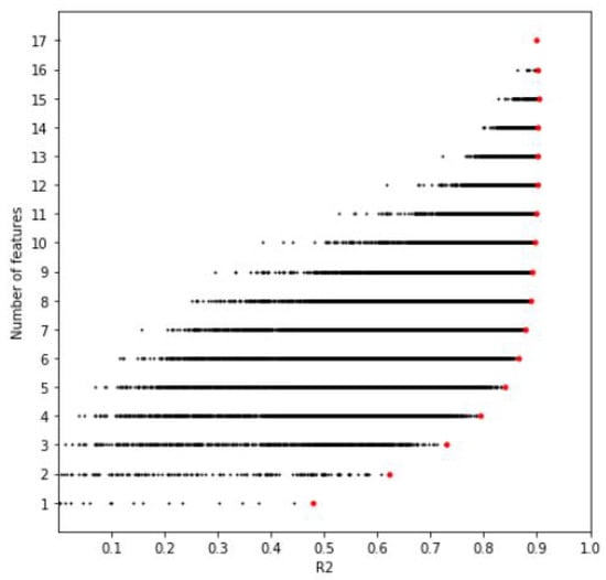
Figure 16.
Performance of all the subsets of features using Brute Force Search. Red dots represent the best performance using a specific number of features.
Table 7 presents the features used in each of the best subsets found in the Brute Force Search (corresponding to the red dots in Figure 16). It can be observed that the subset with one feature is the one composed of the feature Jseal, according to the feature with the most significant feature importance found in Experiment 1. The subset with two features is composed of the features Scal and Divide. Those also obtained higher values in feature importance. In general, we can see that the features selected in most of the best subsets are in accord with the ones with the higher values in feature importance (see Figure 13) and correlation value (see Figure 7).
Table 7.
Best subsets performance based on features, MAE, and R2.
One important thing is that the feature SpallJ is only selected in the subsets with 16 and 17 features (see Table 7), even when it has high feature importance (see Figure 13) and high correlation with PCI (see Figure 7). This is explained because it highly correlates with SpallC (see Figure 7). This is because both pathologies are essentially the same, differing only in their location, with SpallC in the corner and SpallJ along the joint.
To validate the best subsets’ performance, we use cross-validation (k = 50) to calculate the R2 and MAE metrics. Table 6 shows the average value of R2 and MAE obtained in those executions. Figure 17 shows the MAE and R2 values obtained in the 50 executions. For up to 10 features, the R2 values are higher than 0.9, and the MAE of the subsets with 15, 16, and 17 features are too similar. We can observe that the models fitted with 12 and 14 features performed worse than the ones with 11 and 13 features, respectively. This can be explained because those models do not include the feature Jseal (see Table 7). In all the cases, except in the ones with 12 and 14 features, the subsets fitted with the subsets of features found with the Brute Force Search outperform the ones found with Sequential Forward Search in terms of R2.
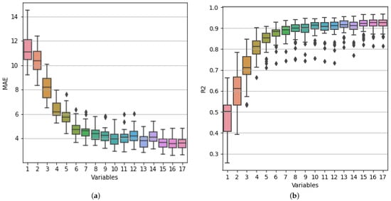
Figure 17.
Performance of the models trained with the subsets of variables found using Brute Force Search based on MAE (a) and R2 (b).
The Friedman test evaluates the null hypothesis of equal ranks for model performance fitted with the subsets of features found with Brute Force Search. The chi-squared statistics obtained for this test were 733.69 and 685.33 for the MAE and R2 measures, respectively. Both chi-squared statistics rejected the null hypothesis with p-values below 0.001. Therefore, certain models’ performances statistically outperform others. Regarding this rejection, the post-hoc Nemenyi test is applied. The critical difference, calculated at 3.5038, is depicted in the significance diagrams, as shown in Figure 18. Figure 18 shows no significant differences in the average rankings, based on MAE, between the models’ performance of the ones fitted with 13, 15, 16, and 17 features because they belong to the same group. On the other hand, based on R2, models fitted with 10, 13, 14, 15, 16, and 17 variables have no significant differences. We can conclude from both statistical tests that we have not found significant differences between the models fitted with 13, 15, 16, and 17 features of the subsets found with Brute Force Search.
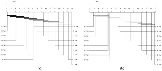
Figure 18.
CD plot of the Nemenyi statistical test comparing the models trained with subsets of variables found using Brute Force Search based on MAE (a) and R2 (b). Groups of algorithms that are not significantly different are connected.
Based on our data and experiments, we can ignore the features Shrink, LaneDF, and PatchS. Shrink is highly correlated, or redundant, with Scal. LaneDF and PatchS have poor feature importance (see Figure 13) and a low correlation with PCI (see Figure 7). We recommend not eliminating SpallJ, although it appears redundant with SpallC; they complement each other because they represent the same pathology but in different locations.
5. Discussion
Although some studies have analyzed the impact that some variables have on the PCI [,], they do not justify why these variables were used. This document presents a sensitivity analysis of the various types of damage used in PCI calculation. Identifying the most significant damages in the PCI calculation offers several benefits. Firstly, it can spur further research into automating PCI calculations, focusing on recognizing the most critical damages. For example, by the use of computer vision such as the work done in [,,,,,]. Additionally, if reducing the number of evaluated damages does not substantially impact the PCI’s numeric value, the evaluation process can be expedited, leading to time and cost savings.
Recently, models based on neural networks, such as deep learning, have become popular because of their robustness in solving difficult problems. However, they are also known as black box models because it is difficult to understand how the predictions are made and what variables have a bigger contribution to the model. In this sense, we decided to use regression models based on decision trees; these models fall into the category of white box models because it is easy to understand how predictions are made and also to identify the feature importance of the variables, which is crucial in a sensitivity analysis.
From the analysis presented in this document, it was possible to verify that some types of damage significantly impact the value of the PCI. To improve the reading, in this section, we will use the following abbreviations: FI for feature importance and C for correlation. The sealing of the joints, Jseal (FI = 0.33 and C = 0.69), is the damage we found as the most significant, and it is the one that creates the best model with only one feature. This damage is usually one of the first to appear, mainly due to the poor quality of the materials used or errors in their placement. Naturally, once the sealing has been lost, the damages that subsequently occur are related to some type of cracking, such as longitudinal and transverse cracking, LinCrk (FI = 0.15, C = 0.70), and corner cracking, Corner (FI = 0.07, C = 0.59), which frequently occur, especially when the slabs begin to lose support, a situation that is commonly generated by the phenomenon of pumping when water enters through poorly sealed joints or those where the seal has been lost. This cracking type is commonly followed by dividing slabs into four or more parts, Divide (FI = 0.10, C = 0.56). Another fairly frequent damage is superficial cracking, Scal (FI = 0.09, C = 0.46), mainly due to excessive concrete handling when giving it the final finish. However, this type of damage is not critical from a structural point of view. However, rather than an aesthetic issue, it must be taken into consideration that, in the long term, delamination or detachment of the concrete could be generated in some superficial areas. Other damages that have a high impact on the PCI were spalling in corners, SpallC (FI = 0.06, C = 0.65), and joints, SpallJ (FE = 0.04, C = 0.64), which are somehow also related to the loss of sealing in the joints since spalling is frequently produced by the inclusion of incompressible materials in the joint space where the seal has previously been damaged or lost, giving rise to the fracturing of the concrete in the adjacent areas by restricting the thermal deformations of the slab, generating concentrations of stresses and subsequent breakage in the areas where the incompressible material is found. Those damages have a high impact on PCI. Therefore, considering that some types of failure significantly impact the PCI, we consider that these variables could be used to estimate the PCI with reasonable precision. As mentioned above, although cracking can be caused by loss of support of the slab, it is also common for either repeated loads or inadequate slab thicknesses to result in cracked slabs, which would happen regardless of sealing damage since the cracking, in principle, would be due to a bad design or a poor quality of the materials used.
From what has been discussed so far, it is evident that some damages occur more frequently than others, giving rise to these having a more significant impact on the PCI, as expected. This can lead us to consider a regression model that considers only some variables, which allows us to obtain the PCI in an automated manner. We did not find a statistical difference in terms of mean absolute error and the coefficient of correlation when using a model trained with 13 features compared with the model trained with all 17 features. Considering the analysis carried out using the SFS and BFS methods, one could think in the first instance of using only 13 variables and ignoring Shrink, LaneDF, SpallJ, and PatchS, resulting in R2 and MAE values corresponding to 0.91 and 3.76, respectively.
Similarly, other possibilities can be studied; that is, the reader will be able to decide the number of variables to use, taking into account the change in the value of R2 and MAE, being able to accept more significant errors by reducing the number of variables involved, and taking into consideration other possible errors inherent to the method, which include errors in the assessment of damage by the evaluator and other interruptions, such as traffic, which sometimes prevents measurements from being adequately carried out. In addition, we can fit a model using only eight damages and obtain an MAE value equal to 4.35 and R2 equal to 0.89. These values are quite similar to the ones obtained with the model fitted with all 17 features: 3.56 and 0.92 in MAE and R2, respectively. This error could be accepted, which, in principle, seems reasonable if other errors related to the evaluator’s expertise or other impediments that frequently result in the zones are considered. For example, parked vehicles that make it impossible to adequately observe and measure the pavement’s damage or the traffic intensity on certain roads significantly complicate measuring and classifying the damage.
It should be noted that understanding that the sealing of joints and the different types of cracks are the issues that most impact the PCI is advantageous since new image analysis technologies could be applied to recognize and classify cracks, which could lead to automating the process of calculating the PCI using a camera mounted in a vehicle and performing the subsequent processing of the images to determine the percentages of damage, which would later be used to calculate the PCI, similar to [,,,,,].
6. Conclusions
This document presents the results of a sensitivity analysis to evaluate the impact of different damages on calculating the Pavement Condition Index (PCI) for rigid pavements. The prediction models employed (Decision Tree, Extra Trees, Random Forest, Ada Boost, and Gradient Boosting) have all yielded successful outcomes, instilling confidence in the robustness of our approach. Among these, the Extra Trees model demonstrated the best performance, achieving a Mean Absolute Error (MAE) of 3.56% and a correlation coefficient (R2) of 0.92 when utilizing all 17 available variables.
The analysis utilized correlation metrics and feature importance assessments to determine the significance of each type of damage. Additionally, we conducted sensitivity analyses through Sequential Forward Search and Brute Force Search techniques, comparing the effects of different subsets of features on the models’ training. Notably, no significant statistical differences in MAE and R2 were found when models trained with 13 features were compared with those trained with all 17 features.
The most impactful damages on PCI prediction were identified as loss of sealing in joints, longitudinal and transversal cracking, divided slab, scaling/map cracking/crazing, corner crack, spalling at corners, and punchout. Conversely, damages such as shrinkage cracks, land/shoulder drop-off, and small patching were found to be less significant. Interestingly, a model utilizing only eight of these damages still achieved an MAE of 4.35 and an R2 of 0.89, values closely approximating those obtained with the complete set of features.
Considering the above, one could consider using only eight variables to determine the PCI, in addition to the fact that these variables are favored for their detection by computer-vision technology, allowing the detection and quantification of damages in the field to be automated. In addition to the above, this study shows the variation of the MAE when an increasing number of variables are used, from the one with the most significant impact to the one with the most negligible impact, which will help other researchers improve their criteria in an automation process since it allows them to know which variables can be implemented and, if applicable, which ones can be omitted, having a clear idea of the possible magnitude of the impact on the PCI in terms of the MAE.
Opting not to include certain damages in the model resulted in a slight increase in prediction error. However, this approach can significantly reduce both the time and cost associated with pavement evaluation, offering a promising avenue for operational efficiency. This flexibility allows stakeholders to balance prediction accuracy and operational efficiency, facilitating automated pavement assessments using computer-vision technology and reducing costs related to damage determination.
Author Contributions
Data curation, A.P. and C.N.S.; formal analysis, A.P., C.N.S., and J.V.; funding acquisition, A.P. and C.N.S.; investigation, A.P., C.N.S., and J.V.; methodology, A.P., C.N.S., and J.V.; project administration, C.N.S.; resources, A.P.; software, A.P., C.N.S., and J.V.; supervision, C.N.S.; validation, A.P., C.N.S., and J.V.; visualization, A.P. and J.V.; writing—original draft, A.P., C.N.S., and J.V. All authors have read and agreed to the published version of the manuscript.
Funding
Jonás Velasco is partially supported by the Chairs Program of the National Council of Humanities, Science and Technology (CONAHCYT) project 2193.
Data Availability Statement
The data presented in the study are openly available in Mendeley Data at https://data.mendeley.com/datasets/mnhn6xvbrg/1 (accessed on 4 September 2024), DOI: 10.17632/mnhn6xvbrg.1.
Acknowledgments
The authors thank the General Directorate of Public Works of the Municipality of León, Guanajuato, for providing the database used in this article. The authors also thank Universidad Panamericana for its support in this research.
Conflicts of Interest
The authors declare no conflicts of interest.
References
- Yoder, E.J.; Witczak, M.W. Principles of Pavement Design; John Wiley & Sons: Hoboken, NJ, USA, 1991; pp. 80–85. [Google Scholar]
- AASHO. Interim Guide for Design of Flexible Pavement Structures; AASHO American Association of State Highway and Transportation Officials: Washington, DC, USA, 1961. [Google Scholar]
- Ullidtz, P. Pavement Analysis; Elsevier: Amsterdam, The Netherlands, 1987. [Google Scholar]
- Sayers, M.W. The Little BOOK of Profiling: Basic Information about Measuring and Interpreting Road Profiles; Technical Report; University of Michigan, Transportation Research Institute: Ann Arbor, MI, USA, 1998. [Google Scholar]
- Shahin, M.Y. Pavement Management for Airports, Roads, and Parking Lots; Springer: Berlin/Heidelberg, Germany, 2005; Volume 501. [Google Scholar]
- Hawks, N.F.; Teng, T.P. Distress Identication Manual for the Long-Term Pavement Performance Project; SHRP-P-338; National Academy of Sciences: Washington, DC, USA, 1993. [Google Scholar]
- HDM Global. Pavement Management Systems and HDM-4. Available online: http://www.hdmglobal.com/hdm-4-version-2/about-hdm-4/pavement-management-systems-and-hdm-4/ (accessed on 26 August 2024).
- US Army Corps of Engineers. WBDG-Whole Building Design Guide. Technical Manuals (TM). Available online: https://www.wbdg.org/ffc/army-coe/technical-manuals-tm/tm-5-623 (accessed on 18 May 2024).
- AASHTO. Pavement Management Guide, 2nd ed.; American Association of State Highway and Transportation Officials: Washington, DC, USA, 2012. [Google Scholar]
- Shahin, M.Y.; Walter, J.A. Pavement Maintenance Management for Roads and Streets Using the PAVER System; USACERL Technical Report M-90/05; U.S. Army Corps of Engineers: Champaign, IL, USA, 1990.
- Prieto, A.; Guiñez, F.; Ortiz, M.; González, M. Fuzzy inference system for predicting functional service life of concrete pavements in airports. Infrastructures 2022, 7, 162. [Google Scholar] [CrossRef]
- Hosseini, S.A.; Alhasan, A.; Smadi, O. Use of deep learning to study modeling deterioration of pavements a case study in Iowa. Infrastructures 2020, 5, 95. [Google Scholar] [CrossRef]
- Kırbaş, U.; Karaşahin, M. Performance models for hot mix asphalt pavements in urban roads. Constr. Build. Mater. 2016, 116, 281–288. [Google Scholar] [CrossRef]
- Shahnazari, H.; Tutunchian, M.A.; Mashayekhi, M.; Amini, A.A. Application of soft computing for prediction of pavement condition index. J. Transp. Eng. 2012, 138, 1495–1506. [Google Scholar] [CrossRef]
- Issa, A.; Sammaneh, H.; Abaza, K. Modeling pavement condition index using cascade architecture: Classical and neural network methods. Iran. J. Sci. Technol. Trans. Civ. Eng. 2022, 46, 483–495. [Google Scholar] [CrossRef]
- Issa, A.; Samaneh, H.; Ghanim, M. Predicting pavement condition index using artificial neural networks approach. Ain Shams Eng. J. 2022, 13, 101490. [Google Scholar] [CrossRef]
- Yan, K.Z.; Zhang, Z. Research in analysis of asphalt pavement performance evaluation based on PSO-SVM. Appl. Mech. Mater. 2011, 97–98, 203–207. [Google Scholar] [CrossRef]
- Kumar, R.; Suman, S.K.; Prakash, G. Evaluation of pavement condition index using artificial neural network approach. Transp. Dev. Econ. 2021, 7, 20. [Google Scholar] [CrossRef]
- Piryonesi, S.M.; El-Diraby, T.E. Role of data analytics in infrastructure asset management: Overcoming data size and quality problems. J. Transp. Eng. Part B Pavements 2020, 146, 04020022. [Google Scholar] [CrossRef]
- Di Benedetto, A.; Fiani, M.; Gujski, L.M. U-Net-based CNN architecture for road crack segmentation. Infrastructures 2023, 8, 90. [Google Scholar] [CrossRef]
- Hammouch, W.; Chouiekh, C.; Khaissidi, G.; Mrabti, M. Crack detection and classification in moroccan pavement using convolutional neural network. Infrastructures 2022, 7, 152. [Google Scholar] [CrossRef]
- Wasiq, S.; Golroo, A. Smartphone-Based Cost-Effective Pavement Performance Model Development Using a Machine Learning Technique with Limited Data. Infrastructures 2024, 9, 9. [Google Scholar] [CrossRef]
- Gagliardi, A.; Staderini, V.; Saponara, S. An Embedded System for Acoustic Data Processing and AI-Based Real-Time Classification for Road Surface Analysis. IEEE Access 2022, 10, 63073–63084. [Google Scholar] [CrossRef]
- Ai, D.; Jiang, G.; Kei, L.S.; Li, C. Automatic pixel-level pavement crack detection using information of multi-scale neighborhoods. IEEE Access 2018, 6, 24452–24463. [Google Scholar] [CrossRef]
- Zhang, B.; Liu, X. Intelligent pavement damage monitoring research in China. IEEE Access 2019, 7, 45891–45897. [Google Scholar] [CrossRef]
- Suh, Y.c.; Kwon, H.j.; Park, K.s.; Ohm, B.s.; Kim, B.i. Correlation analysis between pavement condition indices in Korean roads. KSCE J. Civ. Eng. 2018, 22, 1162–1169. [Google Scholar] [CrossRef]
- Kwak, P.J.; Kim, D.H.; Kim, S.J.; Jeong, J.H. Development of a non-linear PCI model for homogeneous zones of concrete airport pavements. Proc. Inst. Civ. Eng.—Transp. 2021, 174, 305–319. [Google Scholar] [CrossRef]
- Guo, F.; Zhao, X.; Gregory, J.; Kirchain, R. A weighted multi-output neural network model for the prediction of rigid pavement deterioration. Int. J. Pavement Eng. 2022, 23, 2631–2643. [Google Scholar] [CrossRef]
- Ali, A.; Heneash, U.; Hussein, A.; Eskebi, M. Predicting Pavement Condition Index Using Fuzzy Logic Technique. Infrastructures 2022, 7, 91. [Google Scholar] [CrossRef]
- Ali, A.A.; Milad, A.; Hussein, A.; Yusoff, N.I.M.; Heneash, U. Predicting pavement condition index based on the utilization of machine learning techniques: A case study. J. Road Eng. 2023, 3, 266–278. [Google Scholar] [CrossRef]
- Pérez, A.; Sánchez, C.; Velasco, J. Pavement Condition Index (PCI) Data for 5,271 Urban Roads in León, Guanajuato, Mexico. Mendeley Data. 2024. Available online: https://data.mendeley.com/datasets/mnhn6xvbrg/1 (accessed on 4 September 2024).
- Li, B.; Friedman, J.; Olshen, R.; Stone, C. Classification and regression trees (CART). Biometrics 1984, 40, 358–361. [Google Scholar]
- Álvarez-Pato, V.M.; Sánchez, C.N.; Domínguez-Soberanes, J.; Méndoza-Pérez, D.E.; Velázquez, R. A multisensor data fusion approach for predicting consumer acceptance of food products. Foods 2020, 9, 774. [Google Scholar] [CrossRef] [PubMed]
- Breiman, L. Random forests. Mach. Learn. 2001, 45, 5–32. [Google Scholar] [CrossRef]
- Geurts, P.; Ernst, D.; Wehenkel, L. Extremely randomized trees. Mach. Learn. 2006, 63, 3–42. [Google Scholar] [CrossRef]
- Natekin, A.; Knoll, A. Gradient boosting machines, a tutorial. Front. Neurorobotics 2013, 7, 21. [Google Scholar] [CrossRef]
- Solomatine, D.P.; Shrestha, D.L. AdaBoost. RT: A boosting algorithm for regression problems. In Proceedings of the 2004 IEEE International Joint Conference on Neural Networks (IEEE Cat. No. 04CH37541), Budapest, Hungary, 25–29 July 2004; Volume 2, pp. 1163–1168. [Google Scholar]
- Dhal, P.; Azad, C. A comprehensive survey on feature selection in the various fields of machine learning. Appl. Intell. 2022, 52, 4543–4581. [Google Scholar] [CrossRef]
- Pedregosa, F.; Varoquaux, G.; Gramfort, A.; Michel, V.; Thirion, B.; Grisel, O.; Blondel, M.; Prettenhofer, P.; Weiss, R.; Dubourg, V.; et al. Scikit-learn: Machine Learning in Python. J. Mach. Learn. Res. 2011, 12, 2825–2830. [Google Scholar]
- Team, T. Pandas development Pandas-dev/pandas: Pandas. Zenodo 2020, 21, 1–9. [Google Scholar]
- Hunter, J.D. Matplotlib: A 2D graphics environment. Comput. Sci. Eng. 2007, 9, 90–95. [Google Scholar] [CrossRef]
- Harris, C.R.; Millman, K.J.; Van Der Walt, S.J.; Gommers, R.; Virtanen, P.; Cournapeau, D.; Wieser, E.; Taylor, J.; Berg, S.; Smith, N.J.; et al. Array programming with NumPy. Nature 2020, 585, 357–362. [Google Scholar] [CrossRef]
- Allaire, J. RStudio: Integrated development environment for R; RStudio: Boston, MA, USA, 2012; Volume 770, pp. 165–171. [Google Scholar]
- Demšar, J. Statistical comparisons of classifiers over multiple data sets. J. Mach. Learn. Res. 2006, 7, 1–30. [Google Scholar]
- Calvo, B.; Santafé Rodrigo, G. scmamp: Statistical comparison of multiple algorithms in multiple problems. R J. 2016, 8, 248–256. [Google Scholar] [CrossRef]
- López, J.A.; Morales-Osorio, F.; Lara, M.; Velasco, J.; Sánchez, C.N. Bayesian Network-Based Multi-objective Estimation of Distribution Algorithm for Feature Selection Tailored to Regression Problems. In Proceedings of the Mexican International Conference on Artificial Intelligence, Yucatán, Mexico, 13–18 November 2023; Springer: Cham, Switzerland, 2023; pp. 309–326. [Google Scholar]
Disclaimer/Publisher’s Note: The statements, opinions and data contained in all publications are solely those of the individual author(s) and contributor(s) and not of MDPI and/or the editor(s). MDPI and/or the editor(s) disclaim responsibility for any injury to people or property resulting from any ideas, methods, instructions or products referred to in the content. |
© 2024 by the authors. Licensee MDPI, Basel, Switzerland. This article is an open access article distributed under the terms and conditions of the Creative Commons Attribution (CC BY) license (https://creativecommons.org/licenses/by/4.0/).