Abstract
This study evaluates the impact of measurement campaign duration on wind resource characterization using three MCP (Measure–Correlate–Predict) models: Total Least Squares (TLS), Multiple Linear Regression (LR), and Quantile Gradient Boosting (GB). The analysis is based on data from 30 meteorological masts (nine primary and twenty-one secondary masts) installed worldwide across different terrains, with up to twenty-seven months of concurrent wind measurements between primary and secondary masts. Fixed campaign durations of 3, 4, 5, 6, 9, and 12 months were simulated using moving intervals to quantify the effect of measurement length on mean wind speed estimation. This working framework also serves to represent conditions typical of campaigns where LIDAR systems are used to complement meteorological mast deployments, as LIDAR units generally operate for shorter periods due to frequent relocation as part of broader measurement strategies. Wind speed estimation was assessed through metrics such as Mean Absolute Error (MAE), relative uncertainty, and monthly uncertainty reduction, taking into account terrain complexity and correlation coefficient () between masts. Results indicate that extending the measurement period improves the accuracy and consistency of wind speed estimates, with significant reductions in uncertainty observed after six months. Across sites, the average monthly uncertainty reduction ranges from 0.13% to 0.41% of the mean wind speed per additional month of measurements, depending on terrain complexity and inter-mast correlation. Linear models (TLS and LR) consistently show better performance in terms of error and uncertainty reduction compared to GB. Based on an extensive and diverse MCP dataset covering multiple terrains and locations, this study provides empirically derived monthly uncertainty-reduction benchmarks for campaign-length optimisation under different site conditions, contributing to more reliable wind resource assessments and, consequently, energy yield estimates.
Keywords:
wind resource assessment; measurement campaign optimization; artificial intelligence (AI); measure–correlate–predict (MCP) models; total least squares (TLS); multiple linear regression (LR); gradient boosting (GB); complex terrain analysis; meteorological mast correlation; remote sensing device (RSD); LiDAR; machine learning in wind energy 1. Introduction
Accurate wind resource assessment is fundamental to the financial viability and technical success of wind energy projects. A core component of this process is the design and implementation of meteorological measurement campaigns, which are used to characterize wind speed, wind direction, and temporal variability at the project site [1]. Recent advances in mesoscale and microscale modeling are enabling more comprehensive frameworks that integrate meteorological processes with uncertainty quantification in resource assessment [2]. However, deploying meteorological masts for long durations is both costly and logistically challenging. In practice, these campaigns are often based on meteorological masts supported by LIDAR systems, which provide flexible and height-resolved measurements but typically operate for shorter periods due to frequent relocation as part of broader measurement strategies [3,4].
In the context of wind energy development, accurate site characterization is a critical step in reducing project risk and securing financing. While long-term wind data are ideal for reducing uncertainty in energy yield predictions, such datasets are rarely available at potential project locations. As a result, the industry commonly relies on shorter-term on-site measurement campaigns, often supplemented by regional reanalysis datasets or nearby long-term references. However, the extent to which short-duration measurements can reliably represent long-term wind behaviour—particularly in terms of wind directionality and interannual variability—remains a key source of uncertainty. This challenge is especially relevant in complex terrain, where spatial heterogeneity further complicates resource extrapolation. As such, there is growing interest in optimizing the length of measurement campaigns without compromising the reliability of energy production estimates.
Recent evidence also shows that long-term correction (MCP) of sub-annual on-site campaigns can introduce systematic seasonal biases in mean wind speed, variance and AEP—biases strongly influenced by the chosen reanalysis dataset and MCP method—underscoring the risks of relying on short windows for long-term representativeness [5,6,7].
This study investigates how the duration of on-site measurements affects the accuracy and representativeness of wind resource characterization [8]. The analysis is based on a framework that compares wind data from a primary mast, assumed to have long-term reference records, and a secondary mast, which is considered the target for resource estimation. By evaluating multiple measurement periods of varying lengths—3, 4, 5, 6, 9, and 12 months—the study aims to quantify how extending campaign duration improves the estimation of mean wind speed. Although the analysis is based on mast-to-mast comparisons, the findings are also relevant to LIDAR deployments, whose shorter operational windows make understanding duration-driven uncertainty reductions particularly valuable for practical campaign design.
Following the approach introduced by [9], this study acknowledges that, in addition to correlation coefficients between masts, the directional representativeness of wind roses across different measurement windows is a relevant aspect in a comprehensive assessment. In this work, campaign-length effects are evaluated using rolling one-month windows across the measurement period, so potential seasonal influences are implicitly averaged over many start dates. Therefore, seasonal bias is outside the scope of the present study and is left for future work. In this work, campaign-length effects are evaluated using rolling one-month windows across the measurement period, sampling multiple start dates so that potential seasonal influences are implicitly averaged and reflected in the resulting distribution of errors and uncertainties. As seasonality is not explicitly modelled at the level of individual campaigns, the reported uncertainty–duration relationships should be interpreted as aggregated benchmarks of expected behaviour, rather than as a quantification of the seasonality-driven risk associated with any single, site-specific short campaign.
In line with this scope, the present study is designed as an empirical benchmark of how dispersion-based MCP uncertainty decreases with campaign length, using 10-min mean wind-speed inputs that are consistently available across sites. Variables required to isolate specific physical mechanisms (e.g., stability metrics, turbulence intensity, shear, or thermal stratification) were not uniformly available across the multi-site dataset; therefore, we do not claim causal attribution of the error to individual drivers. Instead, we interpret the observed trends using terrain complexity and inter-mast correlation as practical proxies that summarize the combined effects of flow complexity and representativeness on MCP performance.
It is worth noting that shorter campaigns, especially those under 6 months, may capture only limited seasonal variability and therefore fail to reproduce the dominant wind sectors observed in long-term datasets [8,10,11].
This work extends previous research by analysing 21 primary–secondary mast pairs worldwide, applying three MCP models, and evaluating campaign lengths from 3 to 12 months. Unlike prior studies, we quantify how uncertainty decreases with each additional month of measurement and how this behaviour depends on terrain complexity and inter-mast correlation. Importantly, to the best of our knowledge, no previous study has conducted a formal, data-driven assessment based on a dataset of this size and diversity, nor provided empirically derived monthly uncertainty-reduction factors that can be directly used to define practical benchmarks and minimum campaign durations for bankable wind resource assessments. Although LR, TLS, and GB are established methods, their use is deliberate: we employ widely accepted baselines to isolate the effect of measurement-period length and to benchmark whether a representative ML model (GB) provides a material improvement over TLS, a fast and commonly adopted reference in practice. Accordingly, the contribution is not the introduction of a new MCP algorithm, but the provision of multi-site, empirically derived monthly uncertainty-reduction factors and benchmark ranges stratified by terrain complexity and inter-mast correlation, enabling campaign-length optimisation and minimum-duration guidance. These insights are particularly relevant for hybrid campaigns combining longer mast measurements with shorter-duration standalone LIDAR deployments.
The remainder of this paper is organized as follows: Section 2 introduces the available data used in the study, including meteorological mast configurations and terrain classifications, as well as, details the methodology applied for analysing wind speed using multiple MCP models. Section 3 presents the main results and findings related to the impact of the duration of the measurement campaign on various evaluation metrics. Finally, Section 4 summarizes the key conclusions.
2. Materials and Methods
The following sections provide a detailed description of the data and methodology applied to analyse wind speed estimation at secondary meteorological masts, including the MCP models used and the evaluation metrics considered in this study.
2.1. Available Data
The tests were conducted using nine primary meteorological masts and twenty-one secondary masts. Each wind farm included at least one primary–secondary mast pair, ensuring concurrent measurements at the same site. The considered wind farms are located on different continents worldwide.
All masts were equipped with anemometers and other standard meteorological instruments according to traditional industry configurations. For all masts, the upper measurement height was selected as the main wind speed.
The measurement setup and data structure follow widely used configurations in wind resource assessment studies [12], ensuring comparability and methodological transparency.
The available masts are located across diverse terrains (flat, semi-complex, and complex) within onshore environments. In this dataset, 4 secondary masts are located in flat terrain, 10 in semi-complex terrain, and 7 in complex terrain. Terrain complexity has been considered as an input variable for evaluating the impact of measurement campaign length.
A concurrent period of up to twenty-seven months, whenever possible, was considered between each primary–secondary mast pair to perform the wind speed correlation required for the analysis.
Prior to the MCP analysis, all wind speed and wind direction time series were subjected to a standardized quality-control (QC) procedure combining automated flagging and expert review. Automated QC was performed using the commercial software Windographer [13], applying predefined physical-consistency, sensor-range, variability, and icing-detection rules. Additional manual screening was conducted through visual inspection of time series and cross-checks between sensors and mast levels. For transparency and reproducibility, the complete set of QC rules, thresholds, and typical data-removal impacts is reported in Appendix A (Table A1 and Table A2), together with the final temporal resolution and effective sample size used in the analysis. Due to data-confidentiality constraints, mast-level removal rates and exact post-QC record counts are not disclosed; however, the QC workflow was applied consistently across all masts and measurement windows, and only time series with high data availability were retained for the subsequent analysis.
For each wind farm, the representative wind speed at the primary mast (reference data), without long-term correction, was extrapolated to each secondary mast (target data) using correlations based on daily mean wind speeds measured at both masts.
2.2. Measure-Correlate-Predict Models
This section describes the methodologies applied to compare the results and their uncertainty of the three selected MCP models (measure-correlate-predict). Most MCP methods require a significantly high degree of correlation between the target (secondary mast) and reference data (primary mast). On the other hand, MCP models are mainly considered in two groups as linear and nonlinear models. In this analysis, it has been considered “Multiple Linear Regression” algorithm (LR) [14] and Total Least Squares Method (TLS) [15] as linear models and, on the other hand, “Quantile Gradient Boosting” (GB) algorithm [16] as nonlinear model.
2.2.1. Total Least Squares (TLS) Method
Total Least Squares (TLS) [17] is an extension of the classical least squares approach designed for scenarios where both independent and dependent variables contain measurement errors.
In this paper, TLS is used to characterize the linear wind-speed relationship between the considered primary and the secondary mast in each analysed case.
In the context of meteorological mast correlations, TLS can provide a more reliable estimation of wind-speed relationships between the primary (independent) and secondary (dependent) masts. This results in more robust linear models, particularly when input data exhibit noise or inconsistencies due to measurement quality.
The following equations provide the TLS implementation used for the considered linear fit . TLS is an errors-in-variables regression that estimates m and b by minimizing the orthogonal (perpendicular) distances from the paired observations to the fitted line (in contrast to ordinary least squares (OLS), which minimizes vertical residuals). This closed-form expression corresponds to the classical unweighted orthogonal regression solution, which is mathematically equivalent to the singular value decomposition (SVD)-based TLS formulation described in [18,19].
For N paired samples, we compute the centered scatter terms:
where and denote sample means. The TLS slope is then obtained in closed form as:
and the intercept is:
This estimator accounts for uncertainty in both x and y, which matches the mast-to-mast measurement setting considered in this study. In practice, the TLS correlation was implemented using the commercial software Windographer (UL Solutions) through the Long Term Adjustments module (Correlate Speed submodule) with the Total Least Squares (TLS) algorithm [13].
2.2.2. Quantile Gradient Boosting (GB)
“Quantile Gradient Boosting” (GB) [16,20,21,22] is a supervised, non-linear regression method based on decision trees, where boosting constructs an additive predictor by sequentially fitting weak learners. Given a training sample , the goal is to find a function that minimizes the expected value of a specified loss function :
Boosting approximates by an additive expansion
where denotes the m-th base learner (here, a regression tree). The model is fit in a forward stage-wise manner and updated as
where is the shrinkage (learning-rate) parameter.
In this work, GB is used in its quantile-regression form by selecting the quantile (pinball) loss for a chosen quantile level :
Accordingly, each new tree is fitted to the current pseudo-residuals (negative gradient of the loss), so that successive learners correct the remaining errors of the ensemble [16,20]. GB can estimate conditional quantiles; however, in this study we only used (median) and therefore we do not report prediction intervals.
In practice, the model was trained in R using the lightgbm package in its quantile-regression setting (objective = "quantile") with alpha = 0.50 (i.e., = 0.50) [23]. The hyperparameters were optimized through grid search. The optimization results indicate that the relationship between the wind speeds of the meteorological stations can be determined using a Quantile Gradient Boosting model with num_iterations = 1000, max_depth = 3, learning_rate = 0.1, and num_leaves = 5. The model was trained for each meteorological station by combining the target wind speed at the secondary mast with all wind-speed measurements recorded at multiple heights at the reference mast, yielding a station-specific predictor.
2.2.3. Multiple Linear Regression (LR)
“Multiple Linear Regression” (LR) [14] is a linear model that operates similarly to simple linear regression of the form , but uses more than one independent variable, as described in Equation (8)
where “y” is the response variable, “” are the independent variables, is the intercept, , , …, are the regression coefficients, and is the error term.
In this work, the linear model was fitted using quantile regression at (i.e., the conditional median, P50), consistent with the quantile-based formulation used for the GB model [24,25]. Following Koenker and Bassett [24] and Koenker and D’Orey [26], regression quantiles are defined as solutions to the optimization problem:
where , n is the number of observations, is the vector of predictors for observation i, and is the coefficient vector. Under the linear location-shift model , the corresponding conditional quantile function is [26]:
In practice, the fit was computed in R using the rq function from the quantreg package with its default solver, the modified Barrodale–Roberts algorithm (method=br) [26].
The objective of this model is to identify the best relationship between wind speed at the secondary meteorological station and the speeds at various heights at the primary station.
2.3. Evaluation Metrics for Wind Speed Analysis
The main objective of this section is to describe the metrics used to quantify the accuracy of wind speed estimation at secondary masts based on their correlation with primary masts. These metrics form the basis for the subsequent analysis of the effect of measurement campaign length.
In this paper, two metrics are used:
- Mean Absolute Error (MAE), used to quantify the absolute deviation between measured and estimated wind speeds.
- Wind speed uncertainty (%), defined as the relative dispersion of the estimation error for each variable-length period.
The following subsections describe each metric in detail.
2.3.1. Mean Absolute Error (MAE)
Mean Absolute Error (MAE) [27] is a metric used to evaluate the accuracy of the MCP models by quantifying the average absolute difference between estimated and measured wind speeds at the secondary mast. Smaller MAE values indicate better agreement between MCP estimates and observations.
The standard definition of MAE is:
For consistency with the notation used in this study, the MAE can be equivalently expressed as:
where:
- is the wind speed estimated by the MCP model at sample i.
- is the measured wind speed at the secondary mast for the same sample.
- N is the number of samples within the available period at the secondary mast.
2.3.2. Dispersion-Based Uncertainty (Error Dispersion) in Terms of Wind Speed
In addition to analysing MAE, the dispersion-based uncertainty (error dispersion) in wind speed estimation was computed for each of the considered variable-length periods (3, 4, 5, 6, 9, and 12 months). For this study, dispersion-based uncertainty is defined as the relative standard deviation of the MCP estimation error, normalised by the average wind speed measured at the secondary mast during the available period.
The full expression is:
This can be written more compactly as:
where:
- is the wind speed estimated at the secondary mast by the MCP model for sample i.
- is the measured wind speed at the secondary mast for the same sample.
- is the estimation error at sample i.
- is the mean estimation error:
- is the sample standard deviation of the error series.
- is the mean measured wind speed at the secondary mast over the available period:
- N is the number of available samples within the reference period at the secondary mast.
In this work, “uncertainty” refers to the dispersion of the prediction error (standard deviation) normalized by the mean wind speed. This metric does not quantify systematic over- or underestimation (bias). It is used here to analyse the trend of uncertainty reduction with increasing campaign length, supporting a cost–benefit interpretation of whether adding an additional month of measurements provides a meaningful reduction in error dispersion.
This formulation links the uncertainty directly to the length of the measurement period at the secondary mast and provides a consistent measure for comparing MCP model performance across periods and sites. In this study, uncertainty is used as a dispersion measure of error, defined as the standard deviation of the MCP error series normalized by the mean measured wind speed (dimensionless, in %). This choice is well suited to wind applications because wind-speed errors naturally fluctuate due to turbulence, wake effects, terrain heterogeneity, and sensor-related variability; a dispersion-based metric captures how the stability of the estimation evolves as the campaign length increases, which is the central focus of this work. Normalization ensures comparability across sites and wind regimes, and reporting uncertainty is consistent with common practice in wind resource and performance assessment (e.g., IEC/IEA/MEASNET guidance).
2.4. Uncertainty Reduction Analysis
This subsection describes the post-processing strategy used to analyse how wind speed uncertainty decreases as the measurement campaign length increases. The analysis is performed for all MCP models and is further stratified by two key factors that influence uncertainty behaviour: (i) terrain complexity (flat, semi-complex, and complex), and (ii) the correlation coefficient () between primary and secondary masts. These factors allow the evaluation of how different site conditions affect both the absolute uncertainty levels and the incremental reduction achieved when extending the campaign duration.
2.4.1. Gain in Wind Speed Uncertainty
This analysis quantifies how wind speed uncertainty decreases when the measurement campaign is extended. For each MCP model and for each fixed campaign length, the uncertainty was first computed as defined in Section 2.3.2. The gain in uncertainty is then obtained by calculating the difference in uncertainty between two consecutive campaign lengths (e.g., between 3 and 4 months, 4 and 5 months, etc.).
All available primary–secondary mast pairs were included in this calculation, treating each campaign length as an independent sample. The identity of each mast is not considered relevant in this context, since the objective is to characterize the dependence of uncertainty on campaign duration rather than on site-specific conditions.
The gain therefore represents the average reduction in wind speed uncertainty attributable to adding one additional month of measurements, aggregated across all sites and MCP methods.
2.4.2. Impact of Campaign Length (Terrain, , Linearity)
In addition to evaluating the overall gain in uncertainty, a second analysis was conducted to assess how site characteristics influence the rate at which uncertainty decreases with increasing campaign length. This analysis considers two key factors: terrain complexity and the correlation coefficient () between primary and secondary meteorological masts.
For each fixed campaign duration, uncertainty values were grouped according to the terrain classification of the site (flat, semi-complex, or complex). Averaging the uncertainty across all masts within each terrain class yields representative uncertainty values for every campaign length. The relationship between uncertainty and campaign duration was then examined, and a linear trend was identified. This linear behaviour enables the estimation of uncertainty values for intermediate campaign durations not originally included in the dataset (i.e., 7, 8, 10, and 11 months), which are derived by interpolation.
A parallel analysis was performed based on the correlation coefficient (), focusing exclusively on the TLS model, since LR and GB do not compute correlation coefficients for each campaign length. Uncertainty values were grouped into intervals ranging from 0.80 to 1.00, using increments of 0.05. For each interval, representative uncertainty values were derived for each campaign length, and the corresponding monthly uncertainty reduction was obtained.
This approach allows the influence of both terrain complexity and inter-mast correlation on the uncertainty–duration relationship to be quantified, providing a structured basis for interpreting the results presented in Section 3.
3. Results and Discussion
The following section presents how the measurement campaign length influences wind speed estimation at the secondary mast—based on correlations with the primary mast—across the selected MCP models. The analysis of the impact of measurement campaign length on wind speed has been structured around the key indicators which have been described in previous section (Section 2.3).
3.1. Accuracy of MCP Wind-Speed Estimation (MAE)
MAE was the first metric analysed to assess the impact of the measurement campaign length on the wind speed estimation at the secondary meteorological mast.
Appendix B shows box-and-whisker plots of MAE for all secondary masts, grouped by terrain complexity. For each mast, MAE values aggregate all computed correlations across the MCP methods and the variable-length measurement periods. On the other hand, Figure 1 reports the corresponding minimum–maximum ranges for three representative secondary masts (one per terrain class), highlighting the progressive narrowing of MAE dispersion as the measurement period increases.
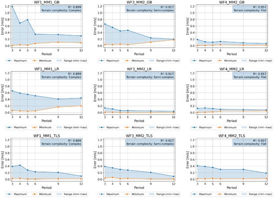
Figure 1.
Wind speed estimation errors as a function of measurement period. Rows correspond to MCP models (GB, LR, TLS), while columns represent terrain complexity classes.
Selected MCP method, terrain complexity and the correlation coefficient () for the concurrent period between mean wind speeds at the primary and secondary masts are included as supplementary variables to support the analysis considering the whole available masts (see Appendix B).
According to the Figure 1 and the Appendix B, the main conclusions are:
- Improved wind speed estimation with longer measurement periods: Wind speed estimates at the secondary mast show lower variability as the length of the measurement period increases (3, 4, 5, 9, or 12 months). MAE values and their dispersion decrease with longer periods regardless of terrain complexity or the correlation coefficient () between mean wind speeds at the primary and secondary masts.
- Error reduction with longer periods: Extending the measurement period to 9 or 12 months leads to significantly lower MAE, reduced dispersion and greater consistency in wind speed estimation at secondary mast, compared to shorter periods (3 to 6 months), enhancing the reliability of the correlations.
- Limited impact of terrain complexity: Terrain complexity has no significant effect on MAE, likely because primary and secondary masts are located within the same site, where topographic influences are inherently incorporated into the correlations.
- Influence of the correlation coefficient (): Higher correlation coefficient () values are linked to lower values of MAE, regardless of considered period length (3, 4, 5, 9, or 12 months). For instance, lower correlation coefficient () values (e.g., ) shows greater variability compared to higher values (e.g., ).
- Lower variability with Total Least Squares (TLS) and Multiple Linear Regression (LR) methods regardless of period length: Total Least Squares (TLS) and Linear Regression (LR) methods show lower dispersion and greater consistency than Quantile Gradient Boosting (GB), even for shorter periods, due to their linear nature, which aligns well with the linear relationship between wind speeds.
3.2. Evolution of Wind-Speed Uncertainty
This section presents the evolution of wind-speed uncertainty as a function of the measurement campaign length. Unlike MAE, uncertainty itself is the metric analysed here; the “gain” (i.e., the reduction in uncertainty when extending the campaign) is derived later in Section 3.3 as part of the post-processing of these values.
Secondary masts are grouped in the same graph based on their wind farm area and the selected MCP method. Different marker types are used according to the correlation coefficient () between secondary and primary masts during their concurrent period.
Figure 2 presents, as an example, a single uncertainty value for each period length for a secondary mast located at one wind farm area, according to the results obtained with TLS, GB, and LR methods. The full set of results is included in Appendix B for all analysed masts.
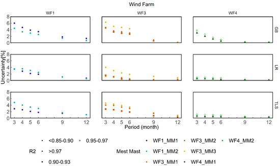
Figure 2.
Wind speed uncertainty at the secondary mast as a function of the daily correlation () between the secondary and primary masts (concurrent period). Single mast only.
In addition, Figure 3 illustrates for the same wind farm area, the uncertainty values obtained for all secondary masts across the different period lengths. Marker types denote the MCP algorithm (GB, LR, or TLS), highlighting its influence on the estimated uncertainty. Appendix C provides the results for all masts.
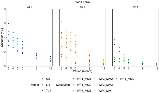
Figure 3.
Wind speed uncertainty at the secondary mast as a function of the correlation model considered between the secondary and primary masts.
After analysing the uncertainty results shown in Figure 2 and Figure 3 and the Appendixes Appendix B and Appendix C, the main conclusions according to all analysed masts are:
- Reduction in wind speed uncertainty with longer measurement periods: Uncertainty decreases systematically as the measurement period is extended by one month or more.
- Influence of correlation strength: Wind speed uncertainty increases as decreases, reducing confidence in the secondary-mast wind speed estimates derived from the primary mast. Higher values lead to more reliable predictions. Figure 4 provides a detailed view of how uncertainty decreases with campaign length for values ranging from 0.80 to 1.00 in 0.05 increments.
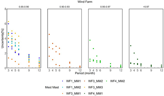 Figure 4. Wind speed uncertainty for 3-, 4-, 5-, 6-, 9-, and 12-month periods, grouped by the correlation coefficient () obtained using the Total Least Squares (TLS) method.
Figure 5 shows the uncertainty results for each secondary mast across all period lengths, grouped by MCP method and categorized by site complexity (flat, semi-complex, or complex) with marker types. This allows visual assessment of the terrain influence on uncertainty levels.
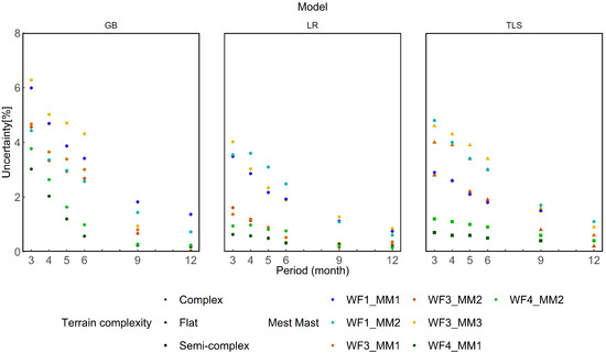
Figure 5.
Wind speed uncertainty as a function of site complexity for each secondary mast.
Based on Figure 5, the main conclusions are:
- Extending the campaign length consistently reduces uncertainty: this behaviour is observed for all MCP methods and terrain types.
- Linear MCP methods achieve lower uncertainty: TLS and LR generally outperform GB, reflecting their stronger ability to represent the underlying linear relationship between wind speeds at the primary and secondary masts.
3.3. Impacts on Uncertainty Reduction
Building on the uncertainty results presented in the previous section, the following analysis examines how the extension of the measurement campaign influences the reduction of wind-speed uncertainty. This assessment is organised around three key aspects:
- The relationship between the measurement campaign length and the resulting reduction in uncertainty.
- The influence of terrain complexity on the uncertainty reduction.
- The influence of the inter-mast correlation coefficient () on the uncertainty reduction.
In the following subsections, the reduction in uncertainty achieved when extending the measurement campaign—interpreted here as the monthly gain in uncertainty—is analysed both globally (Figure 6) and stratified by terrain complexity (Table 1) and by the inter-mast correlation coefficient (Table 2).
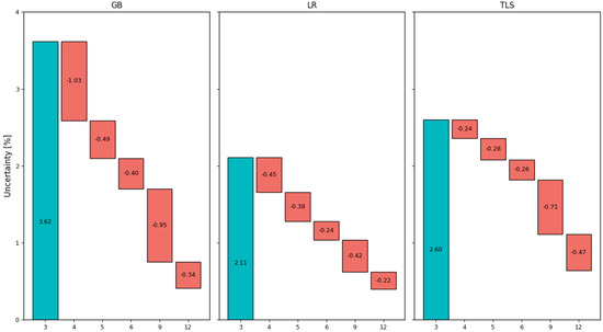
Figure 6.
Wind speed uncertainty gain for 3-month period (blue box), and the uncertainty decrease for the variable-length periods (red box) 4-, 5-, 6-, 9-, and 12-month periods, using Total Least Squares (TLS), Gradient Boosting (GB), and Multiple Linear Regression (LR) methods.

Table 1.
Decrease in uncertainty (Gain) in terms of speed for each month of additional measurement. Methods “Total Least Squares” (TLS), “Multiple Linear Regression” (LR), and “Gradient Boosting” (GB).
Table 2.
Decrease in uncertainty (Gain) in terms of speed for each month of additional measurement. “Total Least Squares” (TLS).
3.3.1. Measured Reduction When Extending Campaign Length
To quantify the effect of extending the measurement campaign on wind-speed uncertainty, a waterfall-style representation was first used to illustrate the reduction achieved as the period length increases. Figure 6 shows the uncertainty decrease for the variable-length periods considered in this study, with uncertainty values aggregated across all secondary meteorological masts and grouped by both campaign duration and MCP method.
A marked reduction in wind-speed uncertainty is observed when extending the campaign from 6 to 9 months. This pronounced drop results from adding three months of data simultaneously, rather than through the one-month increments used in earlier intervals. Once this effect is accounted for, the overall trend remains consistent with a gradual, approximately linear reduction in uncertainty per additional month.
This behaviour is observed across all MCP methods, confirming that campaign duration is the dominant factor governing uncertainty reduction, independently of the specific model used.
The TLS and LR methods exhibit better performance than GB, providing lower uncertainty values and smoother reductions across the analysed periods. Although LR tends to yield slightly lower uncertainties than TLS, the relatively small differences between the two linear approaches highlight their comparable ability to capture the underlying linear relationship between primary and secondary masts.
Building on these measured reductions, a complementary analysis was performed to explicitly evaluate the relationship between wind-speed uncertainty and campaign duration. Uncertainty values for all defined campaign lengths were examined by correlating primary and secondary meteorological mast data. Intermediate, non-calculated periods were estimated by aggregating results in two ways: (i) by terrain complexity for each MCP method, and (ii) by correlation coefficient () for the TLS method only, since LR and GB do not provide values for each measurement window.
This combined analysis reveals an approximately linear relationship between uncertainty and the length of the measurement period. This linearity enables the estimation of uncertainty values for all campaign durations from 3 to 12 months and allows quantifying the monthly reduction in uncertainty, providing a practical basis for defining minimum measurement durations under varying site conditions.
For each campaign length in months, we compute the dispersion-based uncertainty from the test residuals (Equations (13) and (14)). We then fit a linear model using the computed campaign lengths. The reduction rate reported in Table 1 and Table 2 is derived from the fitted slope (negative values indicating decreasing uncertainty with longer campaigns). Intermediate, non-computed campaign lengths are obtained by linear interpolation using the fitted relationship and should be interpreted as an approximation within the analyzed range.
Terrain Influence
Figure 7 together with Figure 8 and Figure 9 illustrate the variation of uncertainty with campaign duration for the three MCP methods (GB, LR, TLS). In all cases, uncertainty decreases linearly with increasing period length, and steeper slopes are observed for complex terrains. In Appendix E, the values used to establish the linear correlations shown in the following figures between uncertainty and measurement-period length, as a function of terrain complexity, are tabulated for the different models (Table A8 and Table A9).
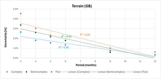
Figure 7.
Uncertainty vs. period length (3–12 months) using the Gradient Boosting (GB) method, grouped by terrain complexity.
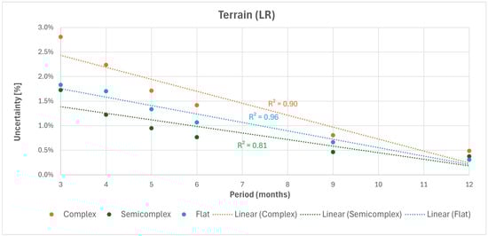
Figure 8.
Uncertainty vs. period length (3–12 months) using the Linear Regression (LR) method, grouped by terrain complexity.
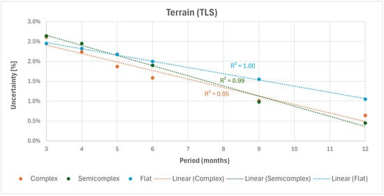
Figure 9.
Uncertainty vs. period length (3–12 months) using the Total Least Squares (TLS) method, grouped by terrain complexity.
Complex terrains exhibit the highest uncertainty levels (reaching 4–5% for 3-month campaigns), while flat terrains show significantly lower values (typically below 1.5% for 12 months). Among the MCP models, TLS provides the strongest linearity, with consistently above 0.95.
Correlation Coefficient Influence
The TLS method also enables grouping uncertainty values according to the correlation coefficient between primary and secondary masts. Figure 10 shows the uncertainty–period relationship stratified by intervals. In Appendix E, the values used to establish the linear correlations shown in the following figures between uncertainty and measurement-period length, as a function of ranges of , are tabulated for the TLS model.
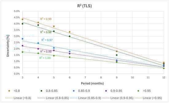
Figure 10.
Uncertainty vs. period length (3–12 months) using the Total Least Squares (TLS) method, grouped by correlation coefficient ranges ().
In Appendix E, the values used to establish the linear correlations shown in the following figures between uncertainty and measurement-period length, as a function of ranges, are tabulated for the different models (Table A12 and Table A13).
Higher correlations correspond to lower uncertainty and better linear fits. For , uncertainty consistently drops below 2% for 12-month campaigns. In contrast, sites with low correlations () show higher uncertainty, especially for short campaigns, and a steeper decline with increasing campaign length.
Across all analyses, both terrain complexity and mast-to-mast correlation significantly influence the uncertainty–period relationship. The dependence on terrain complexity and inter-mast correlation is physically plausible: complex terrain typically increases spatial heterogeneity and flow distortion, reducing the stationarity of the mast-to-mast relationship and requiring longer sampling to achieve representative conditions. Likewise, lower inter-mast correlation indicates that a larger fraction of variability is not explained by the reference mast alone, which is consistent with regime-dependent behaviour (e.g., changing stability/turbulence or directional effects) that may be under-sampled in short campaigns. Therefore, terrain class and can be viewed as practical proxies for the combined influence of these physical drivers on the dispersion of MCP errors. Extending the measurement campaign consistently reduces uncertainty, with the most pronounced improvements observed in complex terrains and in cases with low inter-mast correlation.
3.3.2. Effect of Terrain Complexity on Uncertainty Reduction
This subsection presents a terrain-based analysis of the monthly reduction in wind-speed uncertainty.
Results from all secondary meteorological masts across the nine sites were aggregated according to terrain complexity—flat, semi-complex, and complex—for each MCP method. Table 1 summarises the average monthly reduction in wind-speed uncertainty for each method and terrain class.
The dispersion-based uncertainty decrement values reported are estimated from the tabulated values presented in Appendix E (Table A9, Table A10 and Table A11).
As shown in Table 1, in complex and semi-complex terrains the Gradient Boosting (GB) method provides the largest monthly reductions in wind-speed uncertainty, with values of –0.38% and –0.33%, respectively. TLS exhibits intermediate reductions (–0.21% to –0.25%), while LR yields slightly smaller reductions in complex terrain (–0.24%) and clearly lower reductions in semi-complex terrain (–0.13%). For flat terrains, TLS and LR provide comparable monthly reductions (–0.16% and –0.17%, respectively), with GB performing marginally better (–0.23%).
However, it is important to note that the larger reductions obtained with GB do not necessarily reflect superior model performance. GB tends to start from higher baseline uncertainty, meaning that its apparent monthly improvement partially results from correcting a less accurate initial estimation rather than from intrinsically better predictive capability. This behavior is consistent with the way GB learns the relationship: unlike LR and TLS, which fit a single global linear mapping, GB builds the prediction progressively and can therefore be more sensitive to limited and potentially unbalanced training samples. Therefore, the higher baseline uncertainty is more plausibly linked to terrain- and sample-driven variability than to inappropriate tuning.
The observed underperformance of GB relative to linear baselines can be explained by the modelling context of this benchmark. The predictor set is intentionally limited to concurrent wind speed, for which the dominant cross-mast relationship is often close to linear; consequently, the additional flexibility of boosting may not translate into improved generalization. Moreover, short training windows and rolling-window evaluation reduce the effective sample size (due to temporal autocorrelation) and may introduce regime shifts between training and test windows. Rolling windows are used to sample multiple start dates, so that the influence of seasonal variability is implicitly included in the dispersion of outcomes across windows, albeit without explicit attribution to individual seasons. Under these conditions, more flexible models can exhibit higher variance and sensitivity to sampling variability, whereas linear models tend to remain more stable.
3.3.3. Effect of Inter-Mast Correlation () on Uncertainty Reduction
An analogous analysis was performed considering the correlation coefficient () between primary and secondary meteorological masts, specifically for the Total Least Squares (TLS) method. As described in the previous section, a linear relationship was identified between wind-speed uncertainty and the measurement-period length as a function of . This analysis could not be replicated for Multiple Linear Regression (LR) or Gradient Boosting (GB), since these methods do not compute a correlation coefficient for each variable-length period.
In this case, wind-speed uncertainty results were categorized into intervals from 0.80 to 0.95 in increments of 0.05, enabling the stratification of uncertainty values from all secondary masts across the nine sites according to the strength of the inter-mast correlation.
Table 2 presents the monthly decrease in wind-speed uncertainty for each interval, highlighting the strong dependence of uncertainty reduction on correlation quality. The dispersion-based uncertainty decrement values reported in Table 2 are estimated from the tabulated values presented in Appendix E (Table A14).
Table 2 shows that sites with lower correlation between the primary and secondary meteorological masts require longer measurement periods to reach comparable uncertainty levels. The lowest uncertainty values occur for above 0.95, while increased dispersion and higher uncertainty persist for values around 0.95, and especially for values below 0.90, where uncertainty becomes markedly more variable for shorter periods.
These results confirm that the monthly gain in uncertainty reduction depends strongly on the strength of the inter-mast correlation, ranging approximately between 0.14% and 0.41% per month in every case analyzed.
4. Conclusions
This study evaluates how the duration of a wind measurement campaign influences the accuracy and uncertainty of MCP-based wind speed estimation at secondary meteorological masts. The analysis was carried out across nine sites with different terrain characteristics, using a total of 21 pairs of primary-secondary meteorological masts, and applying three MCP methods—Total Least Squares (TLS), Multiple Linear Regression (LR), and Gradient Boosting (GB). The assessment incorporates two key indicators, MAE and wind-speed uncertainty, and examines how both terrain complexity and the inter-mast correlation coefficient affect the monthly reduction in uncertainty, thereby providing a comprehensive view of how site conditions modulate the benefits of extending campaign length.
The results show that longer measurement campaigns consistently improve MCP accuracy, with MAE values decreasing and their dispersion narrowing as the campaign length increases. This behaviour is observed regardless of terrain complexity or MCP method, although linear methods (TLS and LR) exhibit lower variability and greater robustness than the non-linear GB model. This result delineates the short-sample, limited-input regime in which linear MCP methods remain a robust baseline and indicates that any systematic advantage of non-linear ML models is more likely to emerge with longer concurrent records and richer predictors. The present analysis relies on wind-speed data that are consistently available across all sites; with this input set, the causal contribution of individual physical mechanisms (e.g., stability, turbulence intensity, wake/terrain-induced effects) to the observed error variability cannot be isolated. Nevertheless, the dependence on terrain complexity and inter-mast correlation is physically plausible: complex terrain typically increases spatial heterogeneity and flow distortion, reducing the stationarity of the mast-to-mast relationship and requiring longer sampling to achieve representative conditions, whereas lower inter-mast correlation indicates that a larger fraction of variability is not explained by the reference mast alone. Accordingly, terrain class and can be interpreted as practical proxies for the combined influence of these physical drivers on the dispersion of MCP errors. Within this scope, the reduction of uncertainty with longer measurement periods is mainly statistical: longer campaigns improve the representativeness of observed conditions and stabilize MCP fitting, thereby reducing error dispersion across rolling windows. Mechanism-resolving attribution using additional covariates remains a clear direction for future work.
Regarding uncertainty, the results demonstrate a systematic reduction in wind-speed uncertainty with increasing campaign duration. Uncertainty decreases progressively from 3 to 12 months and is strongly influenced by both terrain complexity and the correlation between primary and secondary masts. Linear models again outperform GB, providing more stable uncertainty estimates across varying site conditions.
The analysis of the monthly gain in uncertainty reduction—obtained by quantifying the decrease in uncertainty when extending the campaign—reveals representative ranges between approximately 0.14% and 0.41% per additional month, depending on terrain type and inter-mast correlation. Terrain-based results show that GB provides the largest reductions in complex and semi-complex terrains, followed by TLS, while LR yields smaller reductions in these terrain classes. For flat sites, TLS and LR behave similarly, while GB yields marginally higher reductions. TLS provides typical reductions of 0.21–0.25% in complex and semi-complex terrains and 0.16% in flat terrains, offering practical reference values for campaign-length optimisation.
Rather than reiterating the general principle that longer campaigns reduce uncertainty, the added value of this work lies in quantifying the marginal monthly uncertainty reduction and demonstrating how these rates vary with terrain complexity and inter-mast correlation, providing empirical reference ranges for campaign-length decisions.
Correlation-based analysis confirms that sites with lower require longer campaigns to reach comparable uncertainty levels. The lowest uncertainty is obtained for correlations above 0.95, while increased dispersion persists at values around 0.95 and particularly below 0.90, especially for shorter campaign durations.
Overall, the combined analysis of MAE, uncertainty evolution, and the derived monthly gain demonstrates how terrain characteristics and inter-mast correlation jointly govern the rate at which uncertainty decreases as the measurement campaign is extended. Based on extensive multi-site empirical evidence, the study provides actionable guidance for selecting appropriate campaign lengths and improving the robustness of MCP-based wind resource assessments, ultimately supporting more reliable project development and energy yield evaluation.
A limitation is that the analysis does not quantify the systematic risk of incomplete annual coverage for any single short campaign (e.g., missing a high-wind season), nor does it provide season-specific uncertainty curves. Therefore, the benchmarks describe average expected behaviour over many possible start dates, and site-specific seasonal-bias risk requires additional stratified analysis. Because the analysis is based on aggregated errors over multiple rolling campaign windows, the sign of the error is not preserved in a consistent manner across realizations. Consequently, bias-related metrics are not robustly defined within this framework and are left for future work based on fixed-reference MCP formulations.
Future work could extend the analysis beyond one-year measurement windows to better capture inter-annual variability and its effect on the uncertainty–duration relationship. Future work should also explicitly quantify seasonal bias by stratifying rolling windows by season (or by annual-coverage metrics) and evaluating whether short-campaign uncertainty differs systematically depending on the months sampled. Expanding the dataset to include additional sites—particularly spanning a broader range of terrain complexity—and extending it with longer concurrent records would enable re-training and re-assessment of ML models under larger effective sample sizes, thereby testing whether non-linear methods provide consistent gains beyond the short-campaign regime analysed here. Targeted analyses in locations with distinctive or “extreme” regimes (e.g., bimodal wind distributions, pronounced vertical shear, strong diurnal contrasts, or persistent stability transitions) would provide a robust test of whether the observed behaviours persist under challenging atmospheric conditions.
In addition, while this work focuses on a dispersion-based uncertainty metric to quantify how the spread of estimation errors contracts with added months of data, future studies could incorporate complementary error components (e.g., systematic offsets) and alternative outcomes. Finally, incorporating additional variables beyond mean wind speed—such as temperature, turbulence intensity, and other operationally relevant indicators—would enable assessing whether extending the measurement campaign by an additional month yields materially improved characterization of conditions linked to turbine loading and potential adverse effects over the asset lifetime.
When intermediate, non-computed campaign lengths are inferred, future work should also evaluate whether the assumed linear relationship holds across regimes and durations, and whether non-linear or piecewise trends provide a better description.
Author Contributions
Conceptualization, A.A.M., A.D.C.M. and A.L.E.; methodology, A.A.M., A.D.C.M., O.Á.P.-A., R.L.G. and P.H.F.V.; software, A.P.T.N.; formal analysis, O.Á.P.-A., P.H.F.V. and A.P.T.N.; investigation, O.Á.P.-A. and P.H.F.V.; resources, O.Á.P.-A. and P.H.F.V.; data curation, O.Á.P.-A. and P.H.F.V.; writing—original draft preparation, O.Á.P.-A.; writing—review and editing, A.A.M., A.D.C.M., O.Á.P.-A., P.H.F.V., A.P.T.N., R.L.G. and A.L.E.; supervision, A.L.E. All authors have read and agreed to the published version of the manuscript.
Funding
This research received no external funding.
Institutional Review Board Statement
Not applicable.
Informed Consent Statement
Not applicable.
Data Availability Statement
The data presented in this study are confidential and cannot be shared.
Conflicts of Interest
Alejandro Abascal Mendez and Ana Del Castillo Martín are employees of Iberdrola Renewable. The remaining authors declare no conflicts of interest.
Abbreviations
The following abbreviations are used in this manuscript:
| LR | Linear Regression |
| TLS | Total Least Squares |
| MCP | Measure–Correlate–Predict |
| GB | Gradient Boosting Regressor |
| MAE | Mean Absolute Error |
| AEP | Annual Energy Production |
| RSD | Remote Sensing Device |
| LIDAR | Light Detection and Ranging |
| STD | Standard Deviation |
| Coefficient of Determination | |
| WF | Wind Farm |
| MM | Meteorological Mast |
| QC | Quality Control |
| LT | Long-Term |
| SpMCP | Wind speed predicted by MCP |
| SpMEAS | Measured wind speed |
Appendix A
Table A1.
Quality-control (QC) rules applied to the mast datasets and typical data removal impact (windographer-based workflow).
Table A1.
Quality-control (QC) rules applied to the mast datasets and typical data removal impact (windographer-based workflow).
| QC Category | Variable | QC Rule/Threshold |
|---|---|---|
| Sensor malfunction/stuck signal | Wind speed | Constant average value over ≥ 3 consecutive 10-min records |
| Physical consistency | Wind speed | Max < Mean or Mean < Min |
| Sensor range/gross errors | Wind speed | Negative values or values outside sensor range |
| Plausible limits | Wind speed | Mean outside 0–40 m·s−1 |
| Variability check | Wind speed | Std ≤ 0, or Std > 3 m·s−1 when Mean ≥ 10 m·s−1 |
| Sensor malfunction/stuck signal | Wind direction | Constant direction over ≥ 9 consecutive 10-min records |
| Sensor range | Wind direction | Direction outside 0–360° |
| Physical variability | Wind direction | Direction standard deviation ≥ 104° |
| Inter-sensor consistency | Wind direction | Veer between redundant vanes > 1 sector (16-sector discretization) |
Table A2.
Final analysis resolution and effective sample size after QC.
Table A2.
Final analysis resolution and effective sample size after QC.
| Item | Value |
|---|---|
| Native recording resolution | 10 min |
| Analysis time step used for MCP | Daily mean wind speed (derived from 10-min data) |
| Nominal records per day (10-min) | 144 |
| Effective records per month (daily series) | ∼28–31 daily values |
| Typical post-QC data availability | >95% |
| Maximum concurrent period | Up to 27 months |
Appendix B
The following figure presents the complete set of box-and-whisker plots of the Mean Absolute Error (MAE) obtained for all combinations of primary and secondary meteorological masts, considering different terrain complexities (Complex, Semi-complex, and Flat) and correlation coefficients (). Each panel represents the distribution of MAE values for the three regression models across measurement periods of 3, 4, 5, 6, 9, and 12 months.
The plots illustrate how MAE values decrease and stabilize as the measurement campaign length increases, confirming the improvement in wind speed estimation accuracy for longer measurement periods. Moreover, the influence of terrain complexity and correlation strength between masts is evident, with lower values generally associated with higher MAE and greater dispersion.
It is important to note that Figure A1 in the main text presents three representative examples extracted from this comprehensive figure, corresponding to distinct terrain types and correlation levels. These examples were selected to facilitate the interpretation of the general patterns observed in the complete dataset shown here.

Figure A1.
Complete box-and-whisker plots of Mean Absolute Error (MAE) for Total Least Squares (TLS), Quantile Gradient Boosting (GB), and Multiple Linear Regression (LR) models, considering measurement periods of 3, 4, 5, 6, 9, and 12 months for all mast combinations.
Figure A1.
Complete box-and-whisker plots of Mean Absolute Error (MAE) for Total Least Squares (TLS), Quantile Gradient Boosting (GB), and Multiple Linear Regression (LR) models, considering measurement periods of 3, 4, 5, 6, 9, and 12 months for all mast combinations.

Appendix C
The following figure presents the complete set of plots showing the gain in terms of wind speed uncertainty at the secondary meteorological masts as a function of the measurement campaign length. Each subplot represents a wind farm (WF1–WF9) and includes the results for all secondary masts associated with it. The uncertainty values were obtained for the three regression models and are shown across measurement periods of 3, 4, 5, 6, 9, and 12 months.
The results indicate a consistent decrease in uncertainty with increasing measurement campaign duration, highlighting the improved stability and reliability of the wind speed estimation for longer periods. In general, higher correlation coefficients () between the primary and secondary masts correspond to lower uncertainty levels, while the effect of terrain complexity remains secondary compared to the influence of .
It is important to note that Figure A2 in the main text presents three representative examples extracted from this comprehensive figure, corresponding to selected wind farms and correlation levels. These examples were chosen to illustrate the main patterns observed in the complete dataset included here.

Figure A2.
Complete plots of wind speed uncertainty at the secondary meteorological masts as a function of the measurement campaign length, considering all wind farms (WF1–WF9), regression models (TLS, GB, and LR), and correlation coefficients () between primary and secondary masts.
Figure A2.
Complete plots of wind speed uncertainty at the secondary meteorological masts as a function of the measurement campaign length, considering all wind farms (WF1–WF9), regression models (TLS, GB, and LR), and correlation coefficients () between primary and secondary masts.

Appendix D
The following figure presents the complete set of plots showing the wind speed uncertainty at the secondary meteorological masts as a function of the measurement campaign length and the applied correlation model. Each subplot represents a specific wind farm (WF1–WF9), where the different symbols correspond to the MCP algorithms used. The uncertainty values are plotted against the measurement periods of 3, 4, 5, 6, 9, and 12 months.
The results indicate that the uncertainty generally decreases as the correlation between primary and secondary masts improves and as the measurement period increases. Among the tested algorithms, the TLS and LR methods tend to show slightly lower uncertainties and a more consistent reduction trend, whereas GB presents higher dispersion, especially for shorter campaign lengths.
It is important to note that Figure A3 in the main text presents three representative examples extracted from this comprehensive figure, corresponding to selected wind farms and mast pairs. These examples were chosen to illustrate the main patterns observed across all models and measurement periods presented here.

Figure A3.
Complete plots of wind speed uncertainty at the secondary meteorological masts as a function of the measurement campaign length and MCP algorithm (GB, LR, and TLS), for all wind farms (WF1–WF9).
Figure A3.
Complete plots of wind speed uncertainty at the secondary meteorological masts as a function of the measurement campaign length and MCP algorithm (GB, LR, and TLS), for all wind farms (WF1–WF9).

Appendix E
For each fixed campaign duration (3, 4, 5, 6, 10, and 12 months), dispersion-based uncertainty was first computed at the secondary-mast level. To provide a Type Terrain–based synthesis, these mast-level dispersion-based uncertainty estimates were aggregated into a single representative value for each campaign length, terrain type combination. An unweighted aggregation was adopted across sites. As so, as all secondary meteorological masts were assigned equal contribution to the terrain-type estimate. Group metric was defined as the unweighted arithmetic mean of the corresponding secondary-mast results. Therefore, all secondary meteorological masts were assigned equal contribution to the terrain-type estimate.
Next table shows the average dispersion-based uncertainty (%) obtained according to considered methods by campaign length and Type Terrain. Additionally, it is shown the main correlation coefficients obtained from the linear correlation for each Type Terrain.
Table A3.
TLS method: Average speed dispersion-based uncertainty (%) for each measurement period and terrain type.
Table A3.
TLS method: Average speed dispersion-based uncertainty (%) for each measurement period and terrain type.
| TLS Method—Average Sp Dispersion-Based Uncertainty (%) | ||||
|---|---|---|---|---|
| All Type Terrain | Complex | Semi-Complex | Flat | |
| 3 months | 2.6% | 2.6% | 2.6% | 2.5% |
| 4 months | 2.4% | 2.2% | 2.5% | 2.3% |
| 5 months | 2.1% | 1.9% | 2.2% | 2.2% |
| 6 months | 1.8% | 1.6% | 1.9% | 2.0% |
| 7 months | - | - | - | - |
| 8 months | - | - | - | - |
| 9 months | 1.1% | 1.0% | 1.0% | 1.6% |
| 10 months | - | - | - | - |
| 11 months | - | - | - | - |
| 12 months | 0.6% | 0.6% | 0.5% | 1.1% |
Table A4.
TLS method: Correlation coefficients for speed estimation across terrain types.
Table A4.
TLS method: Correlation coefficients for speed estimation across terrain types.
| TLS Method—Correlation Coefficients | ||||
|---|---|---|---|---|
| All Type Terrain | Complex | Semi-Complex | Flat | |
| R2 | 0.99 | 0.95 | 0.99 | 1.00 |
| Scale | −0.0022 | −0.0021 | −0.0025 | −0.0016 |
| Offset | 0.0321 | 0.0305 | 0.0342 | 0.0294 |
Table A5.
LR method: Average speed dispersion-based uncertainty (%) for each measurement period and terrain type.
Table A5.
LR method: Average speed dispersion-based uncertainty (%) for each measurement period and terrain type.
| LR Method—Average Sp Dispersion-Based Uncertainty (%) | ||||
|---|---|---|---|---|
| All Type Terrain | Complex | Semi-Complex | Flat | |
| 3 months | 2.1% | 2.8% | 1.7% | 1.8% |
| 4 months | 1.7% | 2.2% | 1.2% | 1.7% |
| 5 months | 1.3% | 1.7% | 0.9% | 1.3% |
| 6 months | 1.0% | 1.4% | 0.8% | 1.1% |
| 7 months | - | - | - | - |
| 8 months | - | - | - | - |
| 9 months | 0.6% | 0.8% | 0.5% | 0.7% |
| 10 months | - | - | - | - |
| 11 months | - | - | - | - |
| 12 months | 0.4% | 0.5% | 0.4% | 0.3% |
Table A6.
LR method: Correlation coefficients for each terrain type.
Table A6.
LR method: Correlation coefficients for each terrain type.
| LR Method—Correlation Coefficients | ||||
|---|---|---|---|---|
| All Type Terrain | Complex | Semi-Complex | Flat | |
| R2 | 0.89 | 0.90 | 0.81 | 0.96 |
| Scale | −0.0018 | −0.0024 | −0.0013 | −0.0017 |
| Offset | 0.0234 | 0.0316 | 0.0179 | 0.0227 |
Table A7.
GB method: Average speed dispersion-based uncertainty (%) for each measurement period and terrain type.
Table A7.
GB method: Average speed dispersion-based uncertainty (%) for each measurement period and terrain type.
| GB Method—Average Sp Dispersion-Based Uncertainty (%) | ||||
|---|---|---|---|---|
| All Type Terrain | Complex | Semi-Complex | Flat | |
| 3 months | 3.6% | 4.5% | 3.4% | 2.6% |
| 4 months | 2.6% | 3.0% | 2.6% | 1.8% |
| 5 months | 2.1% | 2.3% | 2.2% | 1.6% |
| 6 months | 1.7% | 1.8% | 1.8% | 1.3% |
| 7 months | - | - | - | - |
| 8 months | - | - | - | - |
| 9 months | 0.8% | 1.0% | 0.6% | 0.8% |
| 10 months | - | - | - | - |
| 11 months | - | - | - | - |
| 12 months | 0.4% | 0.6% | 0.3% | 0.3% |
Table A8.
GB method: Correlation coefficients for each terrain type.
Table A8.
GB method: Correlation coefficients for each terrain type.
| GB Method—Correlation Coefficients | ||||
|---|---|---|---|---|
| All Type Terrain | Complex | Semi-Complex | Flat | |
| R2 | 0.89 | 0.82 | 0.93 | 0.90 |
| Scale | −0.0033 | −0.0038 | −0.0033 | −0.0023 |
| Offset | 0.0401 | 0.0470 | 0.0398 | 0.0289 |
The linear correlation coefficients reported in “section paper” correspond to the relationships illustrated in the associated correlation plots shown in the main manuscript. Figure 7 together with Figure 8 and Figure 9 provide a graphical representation of the same linear fits used to derive from the previous tabulated values.
Using the correlation-based relationships identified in the analyzed durations, dispersion-based uncertainty was additionally estimated for the non-explicitly evaluated campaign lengths (7, 8, 10, and 11 months, blue text data) for each method (TLS, LR, and GB). For each Type Terrain, intermediate values were obtained by interpolating the uncertainty–duration trend inferred from the available campaign-length results, yielding a complete sequence of dispersion-based uncertainty metrics across 3–12 months consistent with the observed dependence on campaign length. The results are shown in the following tables.
Table A9.
TLS method: Average speed dispersion-based uncertainty (%) for each measurement period and terrain type.
Table A9.
TLS method: Average speed dispersion-based uncertainty (%) for each measurement period and terrain type.
| TLS Method—Average Sp Dispersion-Based Uncertainty (%) | ||||
|---|---|---|---|---|
| All Type Terrain | Complex | Semi-Complex | Flat | |
| 3 months | 2.6% | 2.6% | 2.6% | 2.5% |
| 4 months | 2.4% | 2.2% | 2.5% | 2.3% |
| 5 months | 2.1% | 1.9% | 2.2% | 2.2% |
| 6 months | 1.8% | 1.6% | 1.9% | 2.0% |
| 7 months | 1.7% | 1.6% | 1.6% | 1.8% |
| 8 months | 1.4% | 1.3% | 1.4% | 1.7% |
| 9 months | 1.1% | 1.0% | 1.0% | 1.6% |
| 10 months | 1.0% | 0.9% | 0.9% | 1.4% |
| 11 months | 0.8% | 0.7% | 0.6% | 1.2% |
| 12 months | 0.6% | 0.6% | 0.5% | 1.1% |
Table A10.
LR method: Average speed dispersion-based uncertainty (%) for each measurement period and terrain type.
Table A10.
LR method: Average speed dispersion-based uncertainty (%) for each measurement period and terrain type.
| LR Method—Average Sp Dispersion-Based Uncertainty (%) | ||||
|---|---|---|---|---|
| All Type Terrain | Complex | Semi-Complex | Flat | |
| 3 months | 2.1% | 2.8% | 1.7% | 1.8% |
| 4 months | 1.7% | 2.2% | 1.2% | 1.7% |
| 5 months | 1.3% | 1.7% | 0.9% | 1.3% |
| 6 months | 1.0% | 1.4% | 0.8% | 1.1% |
| 7 months | 1.1% | 1.5% | 0.9% | 1.1% |
| 8 months | 0.9% | 1.2% | 0.7% | 0.9% |
| 9 months | 0.6% | 0.8% | 0.5% | 0.7% |
| 10 months | 0.6% | 0.7% | 0.4% | 0.6% |
| 11 months | 0.4% | 0.5% | 0.3% | 0.4% |
| 12 months | 0.4% | 0.5% | 0.4% | 0.3% |
Table A11.
GB method: Average speed dispersion-based uncertainty (%) for each measurement period and terrain type.
Table A11.
GB method: Average speed dispersion-based uncertainty (%) for each measurement period and terrain type.
| GB Method—Average Sp Dispersion-Based Uncertainty (%) | ||||
|---|---|---|---|---|
| All Type Terrain | Complex | Semi-Complex | Flat | |
| 3 months | 3.6% | 4.5% | 3.4% | 2.6% |
| 4 months | 2.6% | 3.0% | 2.6% | 1.8% |
| 5 months | 2.1% | 2.3% | 2.2% | 1.6% |
| 6 months | 1.7% | 1.8% | 1.8% | 1.3% |
| 7 months | 1.7% | 2.0% | 1.6% | 1.3% |
| 8 months | 1.4% | 1.6% | 1.3% | 1.1% |
| 9 months | 0.8% | 1.0% | 0.6% | 0.8% |
| 10 months | 0.7% | 0.9% | 0.6% | 0.6% |
| 11 months | 0.4% | 0.5% | 0.3% | 0.4% |
| 12 months | 0.4% | 0.6% | 0.3% | 0.3% |
A monthly decrease in dispersion-based wind-speed uncertainty for each analysis method was derived by quantifying the incremental gain obtained when adding one additional month of measurements across the different terrain types, based on the values provided in the previous tables.
Following the procedure described above, it has been considered to evaluate the impact of the correlation coefficient on measurement-campaign length. The tables below provide the underlying information used to estimate the final reduction in dispersion-based uncertainty associated with extending the measurement period by one additional month.
Table A12.
TLS method: dispersion-based uncertainty (%) for each measurement period and correlation range.
Table A12.
TLS method: dispersion-based uncertainty (%) for each measurement period and correlation range.
| TLS Method— Dispersion-Based Uncertainty (%) | ||||||
|---|---|---|---|---|---|---|
| All | <0.8 | 0.8–0.85 | 0.85–0.9 | 0.9–0.95 | >0.95 | |
| 3 months | 2.6% | 4.4% | 4.0% | 2.8% | 2.3% | 1.7% |
| 4 months | 2.4% | 4.1% | 3.9% | 2.5% | 2.0% | 1.6% |
| 5 months | 2.1% | 3.8% | 3.4% | 2.1% | 1.9% | 1.5% |
| 6 months | 1.8% | 3.4% | 3.0% | 1.8% | 1.6% | 1.3% |
| 7 months | - | - | - | - | - | - |
| 8 months | - | - | - | - | - | - |
| 9 months | 1.1% | 1.8% | 1.5% | 1.1% | 1.0% | 0.9% |
| 10 months | - | - | - | - | - | - |
| 11 months | - | - | - | - | - | - |
| 12 months | 0.6% | 0.9% | 0.8% | 0.7% | 0.6% | 0.4% |
Table A13.
TLS method: Correlation coefficients for the dispersion-based uncertainty relationships across correlation ranges.
Table A13.
TLS method: Correlation coefficients for the dispersion-based uncertainty relationships across correlation ranges.
| TLS Method—Correlation Coefficients ( ranges) | ||||||
|---|---|---|---|---|---|---|
| All | <0.8 | 0.8–0.85 | 0.85–0.9 | 0.9–0.95 | >0.95 | |
| R2 | 0.99 | 0.99 | 0.98 | 0.97 | 0.99 | 1.00 |
| Scale | −0.0022 | −0.0041 | −0.0039 | −0.0023 | −0.0019 | −0.0014 |
| Offset | 0.0321 | 0.0570 | 0.0528 | 0.0333 | 0.0276 | 0.0219 |
The linear correlation coefficients reported correspond to the relationships illustrated in the associated correlation plots shown in the main manuscript. Figure 10 provide a graphical representation of the same linear fits used to derive from the previous tabulated values.
Table A14.
TLS method: dispersion-based uncertainty (%) for each measurement period and correlation range.
Table A14.
TLS method: dispersion-based uncertainty (%) for each measurement period and correlation range.
| TLS Method— Dispersion-Based Uncertainty (%) | ||||||
|---|---|---|---|---|---|---|
| All | <0.8 | 0.8–0.85 | 0.85–0.9 | 0.9–0.95 | >0.95 | |
| 3 months | 2.6% | 4.4% | 4.0% | 2.8% | 2.3% | 1.7% |
| 4 months | 2.4% | 4.1% | 3.9% | 2.5% | 2.0% | 1.6% |
| 5 months | 2.1% | 3.8% | 3.4% | 2.1% | 1.9% | 1.5% |
| 6 months | 1.8% | 3.4% | 3.0% | 1.8% | 1.6% | 1.3% |
| 7 months | 1.7% | 2.8% | 2.6% | 1.7% | 1.5% | 1.2% |
| 8 months | 1.4% | 2.4% | 2.2% | 1.5% | 1.3% | 1.0% |
| 9 months | 1.1% | 1.8% | 1.5% | 1.1% | 1.0% | 0.9% |
| 10 months | 1.0% | 1.6% | 1.4% | 1.0% | 0.9% | 0.8% |
| 11 months | 0.8% | 1.2% | 1.0% | 0.8% | 0.7% | 0.6% |
| 12 months | 0.6% | 0.9% | 0.8% | 0.7% | 0.6% | 0.4% |
References
- National Renewable Energy Laboratory (NREL). Wind Resource Assessment Handbook: Fundamentals for Conducting a Successful Monitoring Program. 2025. Available online: https://docs.nrel.gov/docs/legosti/fy97/22223.pdf (accessed on 24 October 2025).
- Kelly, M. Beyond the First Generation of Wind Modeling for Resource Assessment and Siting: From Meteorology to Uncertainty Quantification. Energies 2025, 18, 1589. [Google Scholar] [CrossRef]
- Clifton, A.; Clive, P.; Gottschall, J.; Schlipf, D.; Simley, E.; Simmons, L.; Stein, D.; Trabucchi, D.; Vasiljevic, N.; Würth, I. IEA Wind Task 32: Wind Lidar Identifying and Mitigating Barriers to the Adoption of Wind Lidar. Remote Sens. 2018, 10, 406. [Google Scholar] [CrossRef]
- Mkhaitari, R.; Mir, Y.; Zazoui, M. Assessing annual energy production using a combination of lidar and mast measurement campaigns. Int. J. Power Electron. Drive Syst. (IJPEDS) 2023, 14, 2398–2408. [Google Scholar] [CrossRef]
- Basse, A.; Callies, D.; Grötzner, A.; Pauscher, L. Seasonal effects in the long-term correction of short-term wind measurements using reanalysis data. Wind. Energy Sci. 2021, 6, 1473–1490. [Google Scholar] [CrossRef]
- Barber, S.; Schubiger, A.; Koller, S.; Eggli, D.; Radi, A.; Rumpf, A.; Knaus, H. The wide range of factors contributing to wind resource assessment accuracy in complex terrain. Wind. Energy Sci. 2022, 7, 1503–1525. [Google Scholar] [CrossRef]
- Sheridan, L.M.; Duplyakin, D.; Phillips, C.; Tinnesand, H.; Rai, R.K.; Flaherty, J.E.; Berg, L.K. Evaluating the potential of short-term instrument deployment to improve distributed wind resource assessment. Wind. Energy Sci. Discuss. 2024, 10, 1451–1470. [Google Scholar] [CrossRef]
- MEASNET. Evaluation of Site-Specific Wind Conditions v3. 2022. Available online: https://www.measnet.com/wp-content/uploads/2022/09/Measnet_Evaluation-of-Site-Especific-Wind-Conditions_v3-1.pdf (accessed on 17 January 2026).
- Liléo, S.; Berge, E.; Undheim, O.; Klinkert, R.; Bredesen, R.E. Long-term correction of wind measurements. State-of-the-art, guidelines and future work. Complexity 2013, 1, 2–3. [Google Scholar]
- IEA Wind TCP. IEA Wind RP-18 (2017/2022 PDF): Floating Lidar Systems—Acceptance Criteria with a Total of 6 Months of Data. 2022. Available online: https://iea-wind.org/wp-content/uploads/2022/12/RP-18-Task-32-Floating-Lidar-Systems.pdf (accessed on 24 October 2025).
- Olsen, B.T.; Thøgersen, M.L.; Bechmann, A.; Svensson, E. The Influence of Seasonal Biases on Long-Term Correction Uncertainty; Technical Report; DTU Wind Energy: Lyngby, Denmark; EMD International A/S: Aalborg, Denmark, 2021. [Google Scholar]
- Artigao, E.; Vigueras-Rodríguez, A.; Honrubia-Escribano, A.; Martín-Martínez, S.; Gómez-Lázaro, E. Wind Resource and Wind Power Generation Assessment for Education in Engineering. Sustainability 2021, 13, 2444. [Google Scholar] [CrossRef]
- UL Solutions. Windographer: Wind Data Analytics and Visualization Solution. Available online: https://www.ul.com/software/windographer-wind-data-analytics-and-visualization-solution (accessed on 16 January 2026).
- Xin, Y.; Su, X. Linear Regression Analysis: Theory and Computing; World Scientific Publishing Co.: Singapore; Hackensack, NJ, USA, 2009. [Google Scholar] [CrossRef]
- Abuín, J.M.R.; Rojo, J.M. Regresión Lineal Múltiple. 2007. Available online: https://www.academia.edu/11124780/Regresi%C3%B3n_lineal_m%C3%BAltiple (accessed on 14 February 2026).
- Friedman, J.H. Stochastic gradient boosting. Comput. Stat. Data Anal. 2002, 38, 367–378. [Google Scholar] [CrossRef]
- Markovsky, I.; Van Huffel, S. Overview of total least-squares methods. Signal Process. 2007, 87, 2283–2302. [Google Scholar] [CrossRef]
- Golub, G.H.; Van Loan, C.F. An Analysis of the Total Least Squares Problem. SIAM J. Numer. Anal. 1980, 17, 883–893. [Google Scholar] [CrossRef]
- Van Huffel, S.; Vandewalle, J. The Total Least Squares Problem: Computational Aspects and Analysis; Frontiers in Applied Mathematics; Society for Industrial and Applied Mathematics: Philadelphia, PA, USA, 1991; Volume 9. [Google Scholar] [CrossRef]
- Bentéjac, C.; Csörgő, A.; Martínez-Muñoz, G. A comparative analysis of gradient boosting algorithms. Artif. Intell. Rev. 2021, 54, 1937–1967. [Google Scholar] [CrossRef]
- Schonlau, M. Boosting. In Applied Statistical Learning: With Case Studies in Stata; Schonlau, M., Ed.; Springer International Publishing: Cham, Switzerland, 2023; pp. 205–235. [Google Scholar] [CrossRef]
- Alonso, Á.; Torres, A.; Dorronsoro, J.R. Random Forests and Gradient Boosting for Wind Energy Prediction. In Hybrid Artificial Intelligent Systems; Onieva, E., Santos, I., Osaba, E., Quintián, H., Corchado, E., Eds.; Springer International Publishing: Cham, Switzerland, 2015; pp. 26–37. [Google Scholar] [CrossRef]
- Ke, G.; Meng, Q.; Finley, T.; Wang, T.; Chen, W.; Ma, W.; Ye, Q.; Liu, T.Y. LightGBM: A Highly Efficient Gradient Boosting Decision Tree. In Proceedings of the Advances in Neural Information Processing Systems; 2017; Volume 30. Available online: https://proceedings.neurips.cc/paper_files/paper/2017/file/6449f44a102fde848669bdd9eb6b76fa-Paper.pdf (accessed on 17 January 2026).
- Koenker, R.; Bassett, G., Jr. Regression Quantiles. Econometrica 1978, 46, 33–50. [Google Scholar] [CrossRef]
- Koenker, R. Quantile Regression; Econometric Society Monographs; Cambridge University Press: Cambridge, UK, 2010. [Google Scholar] [CrossRef]
- Koenker, R.W.; D’Orey, V. Algorithm AS 229: Computing Regression Quantiles. J. R. Stat. Soc. Ser. C (Applied Stat.) 1987, 36, 383–393. [Google Scholar] [CrossRef]
- Willmott, C.J.; Matsuura, K. Advantages of the mean absolute error (MAE) over the root mean square error (RMSE). Clim. Res. 2005, 30, 79–82. [Google Scholar] [CrossRef]


Disclaimer/Publisher’s Note: The statements, opinions and data contained in all publications are solely those of the individual author(s) and contributor(s) and not of MDPI and/or the editor(s). MDPI and/or the editor(s) disclaim responsibility for any injury to people or property resulting from any ideas, methods, instructions or products referred to in the content. |
© 2026 by the authors. Licensee MDPI, Basel, Switzerland. This article is an open access article distributed under the terms and conditions of the Creative Commons Attribution (CC BY) license.