A Comprehensive Evaluation of Turbulence Models for Predicting Heat Transfer in Turbulent Channel Flow across Various Prandtl Number Regimes

Abstract

Turbulent heat transfer in channel flows is an important area of research due to its simple geometry and diverse industrial applications. Reynolds-Averaged Navier–Stokes (RANS) models are the most-affordable simulation methodology and are often the only viable choice for investigating industrial flows. However, accurate modelling of wall-bounded flows is challenging in RANS, and the assessment of the performance of RANS models for heated turbulent channel flow has not been sufficiently investigated for a wide range of Reynolds and Prandtl numbers. In this study, five RANS models are assessed for their ability to predict heat transfer in channel flows across a wide range of Reynolds and Prandtl numbers ($Pr$) by comparing the RANS results with respect to the corresponding Direct Numerical Simulation data. The models include three Eddy Viscosity Models (EVMs): standard $k-ϵ$, low Reynolds number $k-ϵLS$, and $k-\omega SST$, as well as two Reynolds Stress Models (RSMs): Launder–Reece–Rodi and Speziale–Sarkar–Gatski models. The study analyses the Reynolds number effects on turbulent heat transfer in a channel flow at a $Pr$ of 0.71 for friction Reynolds number values of $180,395,640,$ and 1020. The results show that all models accurately predict velocity across all Reynolds numbers, but the accuracy of mean temperature prediction drops with increasing Reynolds number for all models, except for the $k-\omega SST$ model. The study also analyses the $Pr$ effects on turbulent heat transfer in a channel flow with $Pr$ values between $0.025$ and $10.0$. An error analysis is performed on the results obtained from different turbulence models, and it is shown that the $k-\omega SST$ model has the smallest error for the predictions of the mean temperature and Nusselt number for high-Prandtl-number flows, while the low Reynolds number $k-ϵLS$ model shows the smallest errors for low-Prandtl-number flows at different Reynolds numbers. An analytical solution is utilised to identify $Pr$ effects on forced convection in a channel flow into three different regimes: analytical region, transitional region, and turbulent diffusion-dominated region. These regimes are helpful to discuss the validity of the models in relation to the $Pr$. The findings of this paper provide insights into the performance of different RANS models for heat transfer predictions in a channel flow.

1. Introduction

Heat transfer in turbulent channel flow is widely used for the fundamental understanding and modelling of forced convection within ducts due to its simple geometry [1]. Under the condition where the fluid properties remain constant, the energy equation in this configuration becomes decoupled from the momentum equations, and the temperature can be considered as a passive scalar carried by the background fluid motion. The study of scalar transport and its modelling have gained considerable attention in recent decades due to the importance of turbulent transport of passive scalars (not only the temperature, but also humidity, pollutants, or other chemical species) in many industrial applications [2]. However, accurate experimental measurements of near-wall statistics are relatively scarce due to the difficulty of making precise measurements in the presence of large temperature gradients [3]. Numerical simulation provides an alternative means of obtaining useful information on these flows. There are three types of simulations depending on the level of the resolved scales of turbulence: Direct Numerical Simulation (DNS), Large Eddy Simulation (LES), and Reynolds-Averaged Navier–Stokes (RANS) simulations.

DNS resolves the full range of spatial and temporal scales of turbulence by numerically solving the Navier–Stokes equations without any turbulence model. However, the grid resolution of the discretised domain must be of the order of the Kolmogorov length scale $\eta ={({\nu }^3/ϵ)}^{1/4}$, where $ϵ$ is the dissipation rate and $\nu$ is the kinematic viscosity. The LES approach is a compromise between accuracy and computational cost compared to the DNS and RANS methodologies. In LES, the grid resolution only captures the energy-containing large eddies, while the small-scale physics is modelled using sub-grid scale (SGS) models. However, even LES is often computationally expensive for many industrial and environmental flows with very high Reynolds numbers. By contrast, the RANS methodology models all scales of motion and is the most-computationally affordable technique. However, RANS models often exhibit limited accuracy for some flows, especially those involving heat transfer, where turbulence is anisotropic close to solid boundaries. Additionally, RANS models may not capture large-scale unsteady and coherent turbulent structures that significantly affect heat transfer in some cases. The following is a summary of three different simulation methods used to study turbulent heat transfer in channel flow.

The first DNS of a thermal flow was conducted by Kim and Moin [4] at a friction Reynolds number, $R{e}_{\tau }=u_{\tau }h/\nu$ (where h is the channel half-height), of 180 and for Prandtl numbers $Pr$ of 0.1, 0.71, and 2.0. The friction Reynolds number $R{e}_{\tau }$ is a measure of the turbulent behaviour of the flow, and $Pr$ is the ratio of the momentum diffusivity to the thermal diffusivity. In the simulations performed by Kim and Moin [4], Dirichlet boundary condition was specified at the channel walls. Kasagi and Ohtsubo [5,6] carried out DNS for $Pr=0.71$ and $0.025$ at a Reynolds number of $R{e}_{\tau }=150$. They used constant heat flux boundary conditions for both the top and bottom walls instead of a Dirichlet boundary condition. Kawamura et al. [7] extended DNS to a wide range of Prandtl numbers from $Pr=0.025$ to $5.0$ at $R{e}_{\tau }=180$. They examined the Prandtl number dependence of a fully developed turbulent channel flow and reported that the turbulent Prandtl number, $P{r}_t$, is independent of $Pr$ except for $Pr<0.1$. Kawamura et al. [1] also studied the Reynolds number dependence by carrying out fully developed turbulent channel flow simulations at $R{e}_{\tau }=180$ and 395 for $Pr=0.025$, $0.2$, and $0.71$. Statistical quantities such as the temperature variance, turbulent heat flux, and turbulent Prandtl number were obtained, and the effects of the Reynolds and Prandtl numbers were analysed. Abe et al. [8] carried out the turbulent channel flow simulations at Reynolds number values of $R{e}_{\tau }=1020$ with the $Pr=0.025$ and $0.71$ by Kawamura et al. [1].

LES has recently contributed significantly to turbulent heat transfer in channel flows due to the advancement in sub-grid scale (SGS) modelling, such as the dynamic eddy viscosity model proposed by Germano et al. [9]. Moin et al. [10] conducted the first LES with a dynamic SGS model for compressible turbulent flow with scalar transport in a channel flow configuration at $R{e}_{\tau }=165$, considering three different Prandtl numbers ($Pr=0.1,0.71$, and $2.0$). Later, Wang and Pfletcher [11] used the dynamic SGS model to simulate turbulent channel flows with heat transfer for $R{e}_{\tau }=162$ and 187. However, they used isothermal walls with a large temperature difference between the bottom and top walls, instead of the constant heat flux boundary conditions. Wang et al. [12] conducted heat transfer analysis in turbulent channel flows using the dynamic SGS model with both isothermal walls and constant heat flux boundary conditions for Prandtl numbers ranging from 1 to 100 at $R{e}_{\tau }=180$. Subsequently, an LES-based lattice Boltzmann framework was utilized to analyse heat transfer characteristics in turbulent channel flows at $R{e}_{\tau }=180$ for Prandtl numbers of 0.025 and 0.71 [13]. Currently, heat transfer in turbulent channel flow is a benchmark case for the assessment of model performances and the development of new SGS models.

While LES is a promising method for analysing turbulent heat transfer in ducts, it may not always be affordablein industrial calculations due to its high computational cost. In contrast, RANS is a more-computationally affordable option for such applications, but the accuracy of the modelling of wall-bounded flows poses a significant challenge for RANS models. Therefore, it is important to thoroughly assess the capabilities of RANS models and identify their limitations in terms of the prediction of heat transfer characteristics in turbulent channel flows.

To the best of the authors’ knowledge, there has been little research into the assessment of RANS models for heat transfer predictions in turbulent channel flows across various Prandtl number regimes. An algebraic closure for Reynolds-Averaged turbulent scalar-flux was proposed by Abe and Suga [14] for heat transfer in turbulent channel flows, but the model was only assessed at $R{e}_{\tau }=180$ while using different wall boundary conditions. Later, Pozorski et al. [15,16] used heated turbulent channel flow as a wall-bounded test case for velocity scalar probability density function at $R{e}_{\tau }=180$. A detailed investigation of the variation of the Nusselt number with the Reynolds and Prandtl numbers was performed by Wei [17], and the predictions of the correlations proposed in the literature have been compared with the DNS results. Recently, Mathur et al. [18] evaluated the performance of different scalar flux models in the case of low-Prandtl-number flows along with the influence of varying the turbulent Prandtl number on the accuracy of the model predictions. Mollik et al. [19] assessed several RANS modelling methodologies at various Reynolds numbers ($R{e}_{\tau }=180$, 395, 640, and 1020). However, these studies did not systematically analyse the model performance with respect to variations in the Reynolds and Prandtl numbers.

This paper aims to assess the performance of turbulence models in terms of the predictions of the heat transfer characteristics in turbulent channel flow configurations for incompressible fluids with walls subjected to constant heat fluxes for a wide range of $R{e}_{\tau }$ and $Pr$. The information obtained from this exercise is utilised to identify the relative merits and demerits of different RANS turbulence models. In Section 2, the governing equations and flow setup for a channel flow with constant heat flux on the bottom and top walls are presented. This is accompanied by the summary of the parameters ($R{e}_{\tau }$, $Pr$) of the DNS database, which is utilised to assess the performance of the models. In Section 3, the formulations of the Reynolds-Averaged closures for two classes of RANS models, Eddy Viscosity Models (EVMs) and Reynolds Stress Models (RSMs), are presented, as are the wall functions for the velocity and temperature fields. Section 4 presents the predictions of different turbulence models in terms of the first and second moments of the relevant quantities for different values of $R{e}_{\tau }$ and $Pr$, and these predictions are compared with respect to the corresponding quantities extracted from explicitly Reynolds-Averaged DNS data. Finally, conclusions are drawn from the findings of the above analysis in Section 5.

2. Governing Equations and Flow Setup

This study considers fully developed channel flow for incompressible fluids, where the bottom and top walls are uniformly heated by a constant heat flux $q_w$, as illustrated in Figure 1. The sides along the z-axis are taken to be periodic, and the flow direction is aligned with the x-axis; a periodic boundary condition is also imposed in the x direction. The governing equations are non-dimensionalised by the channel half-width h (i.e., $x_i^{*}=x_i/h$), the friction velocity $u_{\tau }=\sqrt{|{\tau }_w|/\rho }$, the kinematic viscosity $\nu$, and the friction temperature $T_{\tau }=q_w/\rho c_p{u}_{\tau }$. The non-dimensionalised governing equations are shown as follows (where $t^{*}=h/u_{\tau }$).

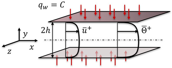
Figure 1. The configuration of turbulent heat transfer in heated channel flow.

Continuity Equation:

$$\frac{\partial {\overline{u}}_i^{+}}{\partial x_i^{*}}=0,$$

(1)

Momentum Equation:

$$\frac{\partial {\overline{u}}_i^{+}}{\partial t^{*}}+{\overline{u}}_j^{+}\frac{\partial {\overline{u}}_i^{+}}{\partial x_j^{*}}=-\frac{\partial {\overline{p}}^{+}}{\partial x_i^{*}}+\frac{1}{R{e}_{\tau }}\frac{{\partial }^2{\overline{u}}_i^{+}}{\partial x_j^{*2}}+\frac{\partial (-\overline{u_i^{+\prime }{u}_j^{+\prime }})}{\partial x_j^{*}}.$$

(2)

In this case, periodic boundary conditions are applied in the x-direction, which can result in energy accumulation in the enclosed heated channel flow system. The bulk mean temperature increases linearly with respect to x for the constant heat flux boundary condition, which contrasts with the periodic boundary condition in the x-direction. To address this issue, a temperature transformation is used, where the energy equation is established based on the local temperature with the removal of temperature at the wall, defined as $\mathsf{\Theta }=T-T_w$. After this transformation, the sink term $-{\overline{u}}_1^{+}/⟨{\overline{u}}^{+}⟩$ arises, which balances the energy input from the bottom and top walls. Here, $⟨{\overline{u}}^{+}⟩$ represents the average velocity over the channel section. More details of the energy equation transformation can be found in [20,21]. With this transformation, the energy equation becomes:

$$\frac{\partial {\overline{\mathsf{\Theta }}}^{+}}{\partial t^{*}}+{\overline{u}}_j^{+}\frac{\partial {\overline{\mathsf{\Theta }}}^{+}}{\partial x_j^{*}}=\frac{1}{R{e}_{\tau }.Pr}\frac{{\partial }^2{\overline{\mathsf{\Theta }}}^{+}}{\partial x_j^{*2}}+\frac{\partial (-\overline{u_j^{+\prime }{\mathsf{\Theta }}^{+\prime }})}{\partial x_j^{*}}-\frac{{\overline{u}}_1^{+}}{⟨{\overline{u}}^{+}⟩}.$$

(3)

The boundary conditions in this case are ${\overline{u}}_i^{+}=0$ and ${\overline{\mathsf{\Theta }}}^{+}=0$ at $y=0$ and $y=2h$. In the momentum equation, the normalized Reynolds stress components $\overline{-u_i^{+\prime }{u}_j^{+\prime }}$, while in the energy equation, the Reynolds heat fluxes $\overline{-u_i^{+\prime }{\mathsf{\Theta }}^{+\prime }}$ are the unclosed terms and, thus, need modelling. A detailed introduction to the models used for these unclosed terms is provided in the next section.

The DNS database of heated turbulent channel flow was established by Kawamura et al. [1,7] over a wide range of $Pr$ (from $0.025$ to $10.0$) and $R{e}_{\tau }$ (from 180 to 1020). The parameters of the DNS database are listed in Table 1, with the available setups marked by a check mark. The RANS simulations are performed using an open-source code called Code Saturne, which is an unstructured finite-volume code designed to compute turbulent flows in industrial applications [22]. This code uses a fractional step method based on a prediction-correction algorithm for pressure/velocity coupling (SIMPLEC) to solve the Navier–Stokes equations for Newtonian incompressible flows, with a second-order central differencing scheme for spatial gradients and an Euler-implicit scheme for time integration [23].

Table 1. A table of available Reynolds numbers and Prandtl numbers from the DNS database of heated turbulent channel flow [1,7,8,14].

$\mathit{Pr}$	0.025	0.5	0.1	0.2	0.4	0.6	0.71	1.0	2.0	5.0	7.0	10.0
$R{e}_{\tau }=180$	✓	✓	✓	✓	✓	✓	✓	✓	✓	✓	✓	✓
$R{e}_{\tau }=395$	✓						✓	✓	✓	✓	✓	✓
$R{e}_{\tau }=640$	✓						✓
$R{e}_{\tau }=1020$							✓

3. Model Formulations for Reynolds-Averaged Closures

As discussed in the Introduction, RANS has the advantage of being more-computationally affordable compared to DNS and LES, and this makes the RANS framework the most-widely used approach in industrial Computational Fluid Dynamics (CFD). It is often the only viable choice for parametric investigations of industrial applications over a wide range of parameters, such as the Reynolds number and Prandtl number. Currently, there are numerous RANS models available that vary in the way Reynolds stresses are modelled. The two main categories are Eddy Viscosity Models (EVMs) and Reynolds Stress Models (RSMs) [24], which are introduced individually in the following subsections.

3.1. Eddy Viscosity Models

Eddy-viscosity-based models, both linear and nonlinear, have become the most-widely used models in turbulence modelling due to their simplicity and efficiency. Among these models, the linear eddy viscosity methodologies are the simplest. These models algebraically evaluate the Reynolds stress using Boussinesq’s hypothesis, which relates the Reynolds stress tensor to the mean velocity gradients in a turbulent flow. Boussinesq’s hypothesis can be expressed as follows:

$$-\overline{u_i^{\prime }{u}_j^{\prime }}={\nu }_t\left(\frac{\partial {\overline{u}}_i}{\partial x_j}+\frac{\partial {\overline{u}}_j}{\partial x_i}\right)-\frac{2}{3}{\delta }_{ij}k.$$

(4)

Here, k is the turbulent kinetic energy, ${\nu }_t$ is the eddy viscosity, which unlike the kinematic viscosity, is not a fluid property and can only be scaled using appropriate velocity and length scales $u_{turb}$ and $l_{turb}$ [25]. In general, $u_{turb}$ is expected to scale as $k^{1/2}$, while $l_{turb}$ can be approximated as $k^{3/2}/ϵ$, where $ϵ$ represents the turbulent dissipation rate. As a result, two-equation models are considered for turbulence modelling. Among these, the $k-ϵ$ and $k-\omega$ models are the most-widely used due to their physical rationale, simplicity, and numerical robustness. In these models, the eddy kinematic viscosity scales as ${\nu }_t=C_{\mu }{k}^2/ϵ$ and ${\nu }_t=C_{\omega }k/\omega$, respectively, where $\omega$ is the specific turbulence dissipation rate, which is closely related to $ϵ$ and provides a measure of the local dissipation rate per unit turbulent kinetic energy.

However, both the $k-ϵ$ and $k-\omega$ models have limitations in RANS simulations. The $k-ϵ$ model is not accurate for complex flows such as swirling flows, recirculating flows, flows with secondary flow features, and flows in non-circular channels. On the other hand, the $k-\omega$ model predictions are highly sensitive to freestream turbulence, and this model without any special treatment can produce unrealistic high values of the turbulent kinetic energy production rate at the stagnation point. To address these limitations, the $k-\omega$ Shear Stress Transport (SST) model was proposed by Menter [26], which combines the advantages of both the $k-ϵ$ and $k-\omega$ models. The use of the $k-\omega$ formulation in the inner parts of the boundary layer makes the model directly usable all the way down to the wall through the viscous sublayer; hence, the $k-\omega SST$ model can be used as a low-Reynolds-number turbulence model. The $k-\omega SST$ formulation replicates the $k-ϵ$ behaviour in the freestream and, therefore, circumvents the common $k-\omega$ problem of being too sensitive to the freestream turbulence.

In the case of scalars, the turbulent scalar flux can be modelled through the Standard Gradient Diffusion Hypothesis (SGDH) [14], which is given as:

$$-\overline{u_i^{\prime }{\mathsf{\Theta }}^{\prime }}=\frac{{\nu }_t}{P{r}_t}\frac{\partial \overline{\mathsf{\Theta }}}{\partial x_i}.$$

(5)

The SGDH provides an algebraic expression for the turbulent scalar flux as the product of the turbulent diffusivity and the scalar gradient. In this expression, the turbulent diffusivity is represented by ${\nu }_t/P{r}_t$ with $P{r}_t$ being the turbulent Prandtl number. For heated turbulent channel flow, $P{r}_t$ typically approaches a value of around $1.0$ near the wall and varies between $0.5$ and $1.0$ away from the wall, except for very low Prandtl numbers ($Pr\le 0.1$) [7]. In our RANS simulations, we adopted a constant value of $P{r}_t=0.71$, which is commonly used as an empirical estimation. The variation of turbulent Prandtl numbers extracted from DNS data [7] shows that $P{r}_t$ varies with the wall-normal distance, but remains of the order of unity and depends on the Prandtl number. Therefore, a single choice of $P{r}_t$ is not straightforward; hence, $P{r}_t=0.7$ is chosen for the RANS simulations conducted here because this is the default value used in most commercial codes. This compromise is made because the effects of $P{r}_t$ on the simulation predictions are not the main objective of this paper. The results can be made to match better with DNS by modifying $P{r}_t$ for a specific case, but this is hardly helpful for practical applications because the optimum value of $P{r}_t$ will not be known a priori. To assess the different turbulence models, we combined the SGDH with various closure techniques for Reynolds stresses. This combination facilitates the comparison of the different models and allows for a more-accurate evaluation of their effectiveness in predicting turbulent heat transfer in a channel flow configuration.

3.2. Reynolds Stress Transport Models

This methodology involves solving modelled transport equations for $R_{ij}=\overline{u_i^{\prime }{u}_j^{\prime }}$. As all components of Reynolds stress are obtained as a part of the solution, RSM models demand a greater computational effort than the previously discussed EVMs. This methodology, nevertheless, can replicate the return to isotropy under decaying turbulence and the limiting behaviour of turbulence under the rapid distortion limit, where turbulence acts as an elastic medium. This category of models is expected to be valid for complex flows.

The modelled transport equation for $R_{ij}$ takes the following form [25]:

$$\frac{D{R}_{ij}}{Dt}=P_{ij}+D_{ij}+{\mathsf{\Pi }}_{ij}+{\mathsf{\Omega }}_{ij}-{ϵ}_{ij}.$$

(6)

The first term on the right-hand side of the above equation represents the production term, indicating a production rate of $R_{ij}$. The second term $D_{ij}$ refers to the molecular diffusion of $R_{ij}$. These two terms $D_{ij}$ and $P_{ij}$ are exact and given by $D_{ij}=\nabla ·\left(\mu \nabla R_{ij}\right)$, $P_{ij}=-R_{im}\partial {\overline{u}}_j/\partial x_m-R_{jm}\partial {\overline{u}}_i/\partial x_m$. The remaining three terms are the transport of $R_{ij}$ due to pressure strain rate interactions (i.e., ${\mathsf{\Pi }}_{ij}$), the transport of $R_{ij}$ due to vorticity (i.e., ${\mathsf{\Omega }}_{ij}$), and finally, the molecular dissipation of $R_{ij}$ (i.e., $-{ϵ}_{ij}$), respectively. The terms $P_{ij}$ and $D_{ij}$ are closed and do not require models in the context of second-moment closure. However, other terms need modelling. Among these, the pressure strain rate interaction term is usually the biggest challenge in the modelling process, where most models differ.

The pressure strain correlation term ${\mathsf{\Pi }}_{ij}$ is typically divided into a rapid part, ${\mathsf{\Pi }}_{ij}^R$, and a slow part, ${\mathsf{\Pi }}_{ij}^S$. The slow part is responsible for the return to isotropy and reduces the anisotropy of the Reynolds stresses. This part represents self-interaction between fluctuating fields:

$$\frac{{\mathsf{\Pi }}_{ij}^S}{ϵ}=f^{\left(1\right)}{b}_{ij}+f^{\left(2\right)}\left(b_{ij}^2-\frac{1}{3}{b}_{kk}^2{\delta }_{ij}\right),$$

(7)

The rapid part captures the interaction of the fluctuating velocity field with the mean velocity field and is dependent on the mean strain rate and rotation rate. The simplest form of the rapid part of most pressure rates of strain models can be expressed as [25,27]:

$$\frac{{\mathsf{\Pi }}_{ij}^R}{ϵ}=f^{\left(3\right)}{\widehat{S}}_{ij}+f^{\left(4\right)}\left({\widehat{S}}_{ik}{b}_{jk}+{\widehat{S}}_{jk}{b}_{ik}-\frac{2}{3}{\delta }_{ij}{b}_{mm}{\widehat{S}}_{mm}\right)+f^{\left(5\right)}\left({\widehat{\mathsf{\Omega }}}_{ik}{b}_{jk}-{\widehat{\mathsf{\Omega }}}_{jk}{b}_{ik}\right).$$

(8)

Here, $b_{ij}=R_{ij}/2k-{\delta }_{ij}/3$ in Equation (7) represents the anisotropy tensor for Reynolds stresses, where ${\delta }_{ij}$ is the Kronecker delta. The quantities ${\widehat{S}}_{ij}$ and ${\widehat{\mathsf{\Omega }}}_{ij}$ in Equation (8) are the normalized mean rate of stain and normalised mean rate of rotation, respectively, defined as ${\widehat{S}}_{ij}=k{\overline{S}}_{ij}/ϵ$, ${\widehat{\mathsf{\Omega }}}_{ij}=k{\overline{\mathsf{\Omega }}}_{ij}/ϵ$.

Several pressure-rate-of-strain models have been proposed for modelling turbulence in fluid flows. One of the earliest and most-widely used pressure-rate-of-strain models is the Launder–Reece–Rodi (LRR) model, which was introduced by Launder et al. [28]. Another example of a Reynolds stress model is the Speziale–Sarkar–Gatski (SSG) model [27]. Table 2 lists the coefficients for the $LRR$ and $SSG$ models. The slow part is closed by using the model proposed by Rotta [29]. The $LRR$ model takes the Rotta coefficient to be constant, whereas $SSG$ model incorporates a dependence of the coefficient on $P/ϵ$, where $P=P_{ii}/2$. Additionally, the $SSG$ model has a non-zero value of $f^{\left(2\right)}$, which leads to the non-linear return to isotropy. The $SSG$ model also considers one of the anisotropy invariants $\eta =\sqrt{(b_{ij}{b}_{ji}/6)}$ of the Reynolds stress tensor. It is worth noting that both the $LRR$ and $SSG$ models are derived models of the original model proposed by Hanjalic and Launder [30].

Table 2. Specifications of the coefficients $f^{\left(n\right)}$ for pressure rate of strain models: $LRR$ and $SSG$.

	${\mathit{f}}^{\left(1\right)}$	${\mathit{f}}^{\left(2\right)}$	${\mathit{f}}^{\left(3\right)}$	${\mathit{f}}^{\left(4\right)}$	${\mathit{f}}^{\left(5\right)}$	Values of Constants
$LRR$	$-2C_R$	0	$4C_2/3$	$2C_2$	$2C_2$	$C_R=1.8$, $C_2=0.6$
$SSG$	$-C_1-C_1^{*}P/ϵ$	$C_2$	$C_3-\sqrt{6}{C}_3^{*}\eta$	$C_4$	$C_5$	$C_1=3.4$, $C_1^{*}=1.8$, $C_2=4.2$, $C_3=0.8$, $C_3^{*}=1.3$, $C_4=1.25$, $C_5=0.4$

3.3. Near-Wall Treatment

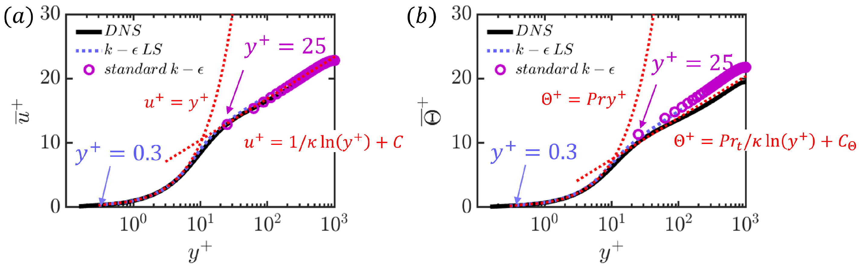
The standard $k-ϵ$ model is a high-Reynolds-number model that is not solved up to the wall. Instead, wall functions are adopted, and the first grid point in the wall-normal direction is typically located in the log-law region. Thus, it can avoid the computational expense of resolving the viscous sublayer. The demarcation point between the buffer layer and the log-law layer is around $y^{+}\approx 30$ [25]. Moreover, the turning point for the thermal boundary layer between the intermediate layer and the log-law layer is around 24.32. Therefore, the first grid point for the current analysis for the standard $k-ϵ$ model is chosen at $y^{+}=25$. The mean velocity profile in Figure 2a shows the existence of the logarithmic region, and the slope of the logarithmic curve is related to the von Karman constant ($\kappa \approx 0.4$) [31]. Similarly, the mean temperature profile in Figure 2b exhibits a logarithmic region with the slope of the logarithmic curve of $P{r}_t/\kappa$.

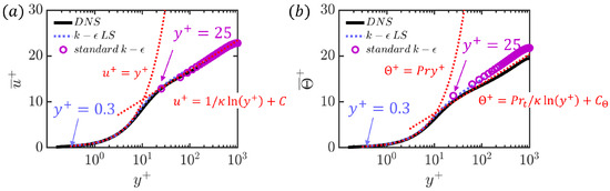
Figure 2. An illustration of the law of the wall for the variation of mean streamwise velocity (a) and mean temperature (b) with different $y^{+}$ values chosen for turbulence models for low-Reynolds-number models and high-Reynolds-number models at $R{e}_{\tau }=180$ and $Pr=0.71$.

Instead of relying on wall functions, a low-Reynolds-number model, such as $k-ϵLS$ [32] and $k-\omega SST$ [26] models, can be used to more-accurately predict near-wall turbulence. These models are solved all the way to the wall, and the near-wall grid resolution needs to be fine enough to resolve the viscous sublayer ($y^{+}<5.0$). In low-Reynolds-number $k-ϵ$ modelling, damping functions are incorporated into the expression for the eddy viscosity and the terms of the transport equations for k and $ϵ$ to account for the near-wall damping. The impact of the choice of the first grid point adjacent to the wall is also illustrated in Figure 2. The standard $k-ϵ$ model employs wall functions and uses a first grid point at $y^{+}=25$, while $k-ϵLS$ model does not use wall functions and is set up with the first grid point at $y^{+}=0.3$.

For the thermal field, the three-layer thermal wall function proposed by Arpaci and Larsen [33] is used instead of resolving the near-wall region. The exact expressions for the three different layers are provided in Table 3. The thermal boundary layer in this heat transfer problem is divided into three layers, which are separated by two turning points: $y_1^{+}={(1000/Pr)}^{1/3}$ and $y_2^{+}=\sqrt{\left(1000\kappa \right)/P{r}_t}$. For the current setup with $\kappa =0.42$ and $P{r}_t=0.71$, the value of $y_2^{+}$ is 24.32 and is independent of $Pr$. The values of the log-law layer for velocity and temperature suggest that the log-law layers for these quantities are nearly aligned. This alignment can also be observed in Figure 2.

Table 3. Three-layer thermal wall function.

Diffusion sublayer	${\mathsf{\Theta }}^{+}=1/Pr{y}^{+}$	$(y^{+}<y_1^{+})$
Intermediate layer	${\mathsf{\Theta }}^{+}=a_2-P{r}_t/\left(2a_1{\left(y^{+}\right)}^2\right)$	$(y_1^{+}\le y^{+}\le y_2^{+})$
Log-law layer	${\mathsf{\Theta }}^{+}=a_3+{Pr}_t/\kappa y^{+}$	$(y_2^{+}<y^{+})$

To conclude, for the heat transfer analysis, a three-layer wall function is used, as the region of the diffusion sublayer is influenced by the Prandtl number. Since a wide range of $Pr$ was considered in this analysis, a mesh that can resolve the diffusion sublayer may not resolve the viscous sublayer and vice versa. The standard $k-ϵ$, $LRR$, and $SSG$ Reynolds stress closures do not integrate up to the wall by design and rely on wall functions by ensuring $y^{+}=25$ for the wall-adjacent grid points, whereas $k-ϵLS$ and $k-\omega SST$ are low-Reynolds-number models, which integrate up to the wall by ensuring $y^{+}<1$ adjacent to the wall and, thus, do not need wall functions.

3.4. A Summary of Selected Turbulence Models

Five different turbulence models, categorised by their type (EVM or RSM) and their requirements in terms of near-wall treatment, are considered here, and these models are summarised in Table 4. The standard $k-ϵ$, $k-ϵLS$, and $k-\omega SST$ models are all EVMs, while $LRR$ and $SSG$ are RSM models. The $k-ϵLS$ and $k-\omega SST$ models are low-Reynolds-number models that do not need wall functions, while the $standard$$k-ϵ$, $LRR$, and $SSG$ models are high-Reynolds-number models that do require the use of a wall function. All of the turbulence models used in this work employ a thermal wall function. Since it covers the entire thermal boundary layer, it allows for flexibility in the location of the first grid point.

Table 4. An overall summary of the Reynolds-Averaged closure models that were selected for assessment.

Models	Reference	Model Type	Wall Function	Thermal Wall Function
standard $k-ϵ$	[32]	EVM	✓	✓
$k-ϵLS$	[34]	EVM		✓
$LRR$	[28]	RSM	✓	✓
$SSG$	[27]	RSM	✓	✓
$k-\omega SST$	[26]	EVM		✓

The values of $y^{*}=y/h$ for the grid points in the wall-normal direction $N_y$ up to the channel half-height for models with a velocity wall function (e.g., standard $k-ϵ$, $LRR$, and $SSG$ models) and without a velocity wall function (e.g., $k-ϵLS$ and $k-\omega SST$ models) are shown in Figure 3 for different values of $R{e}_{\tau }$, which shows that the computational requirement (i.e., number of grid points in the wall-normal direction) is greater for models without wall functions than those with wall functions. Moreover, the computational cost increases with increasing $R{e}_{\tau }$.

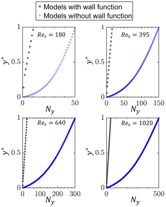
Figure 3. Variations of the normalised wall-normal coordinate of grid points (i.e., $y^{*}=y/h$) with the number of the grid points in the wall-normal direction $N_y$ up to the channel half-height for turbulence models with and without the velocity wall function for different values of $R{e}_{\tau }$. Note that each symbol on the plots represents the cell centre location of the grid point.

Table 5 provides a summary of the computational cost associated with various turbulence models. To demonstrate the differences in the time costs between these models using one core of the CPU (Intel(R) Xeon (R) Silver 4208 CPU @ 2.10 GHz), an example is provided in Table 5 at $R{e}_{\tau }=1020$ and $Pr=0.71$. Compared to the $k-ϵLS$ and $k-\omega SST$ models, the standard $k-ϵ$, $LRR$, and $SSG$ models require less computational cost in the near-wall region due to their adoption of the wall function. The standard $k-ϵ$ model is the least expensive, requiring 0.76 h for the simulation to converge, while $k-\omega SST$ is the most-computationally expensive, requiring 21 h. The mesh requirement is widely different between the standard $k-ϵ$ and $k-\omega SST$ models. The wall-adjacent grid spacing for the standard $k-ϵ$ model is taken to satisfy $y^{+}=25$, whereas the wall-adjacent grid spacing needs to satisfy $y^{+}<1.0$ for the $k-\omega SST$ model, and therefore, a mesh that provides $y^{+}=0.3$ for the wall-adjacent grid points is used. This means the grid points in the wall-normal direction for the $k-\omega SST$ model are 12.5-times those used in the standard $k-ϵ$ model for the grids used in this analysis. Moreover, the $k-\omega SST$ model represents a stiffer system of differential equations than that in the case of the standard $k-ϵ$ model. Therefore, the $k-\omega SST$ model takes longer to reach the steady state than the standard $k-ϵ$ model. The combination of the longer simulation time and the finer grid is responsible for the higher computational cost of the $k-\omega SST$ model simulation in comparison to that using the standard $k-ϵ$ model. Although the $k-\omega SST$ model is more-computationally demanding than the other models, it still offers a significant reduction in computational cost compared to DNS. For example, the number of grid points required for DNS at $R{e}_{\tau }=1020$ and $Pr=0.71$ is 150,000-times larger than that needed for RANS without wall functions and 17.6 million-times larger than that required for RANS models with wall functions. While the computational time of DNS is not available, comparing the number of grid points needed makes it clear that DNS demands significantly more computational resources than RANS.

Table 5. A comparison of the different turbulence models in terms of their computational time at $R{e}_{\tau }=1020$ and $Pr=0.71$.

Models	$\mathit{k}-\mathit{ϵ}\mathit{LS}$	$\mathit{k}-\mathit{\omega }\mathit{SST}$	Standard $\mathit{k}-\mathit{ϵ}$	$\mathit{LRR}$	$\mathit{SSG}$
Time cost (wall clock time)	8.3 h	21.0 h	0.76 h	1.1 h	1.5 h

The boundary conditions for the selected turbulence models are applied as follows. The turbulent kinetic energy is identically zero at the wall due to the no-slip boundary condition. In the case of high-Reynolds-number models that require wall functions and the first grid point to be in the log-layer (e.g., standard $k-ϵ$, $LRR$, and $SSG$ Reynolds stress closures), the cell-averaged value is specified for $ϵ$ as $u_k^3/\kappa y_w$, where $u_k=C_{\mu }^{1/4}{k}^{1/2}$ and $y_w$ is the wall-normal distance of the first grid point adjacent to the wall. For the $k-\omega SST$ model, the wall value of $\omega$ is taken to be $10\times 6\nu /\left[{\beta }_1{\left(y_w\right)}^2\right]$, where ${\beta }_1=0.075$ is a model parameter [26]. For the low-Reynolds-number $k-ϵ$ model, the wall value of $ϵ$ is specified as $2\nu {(\nabla \sqrt{k})}^2$.

4. Results and Discussion

4.1. Heat Transfer Rate in Turbulent Channel Flow for Different Values of Reynolds Number

To investigate the influence of the Reynolds number on the performance of different turbulence models, four different friction Reynolds numbers of 180, 395, 640, and 1020 are considered, each having a Prandtl number of $Pr=0.71$. The obtained mean velocity and mean temperature profiles are compared with the corresponding profiles obtained from the DNS [8,14]. Furthermore, the Reynolds stress distributions are analysed and compared with the corresponding quantities extracted from DNS data to gain a deeper understanding of the performance of the models considered here.

4.1.1. Mean Streamwise Velocity and Temperature Profiles

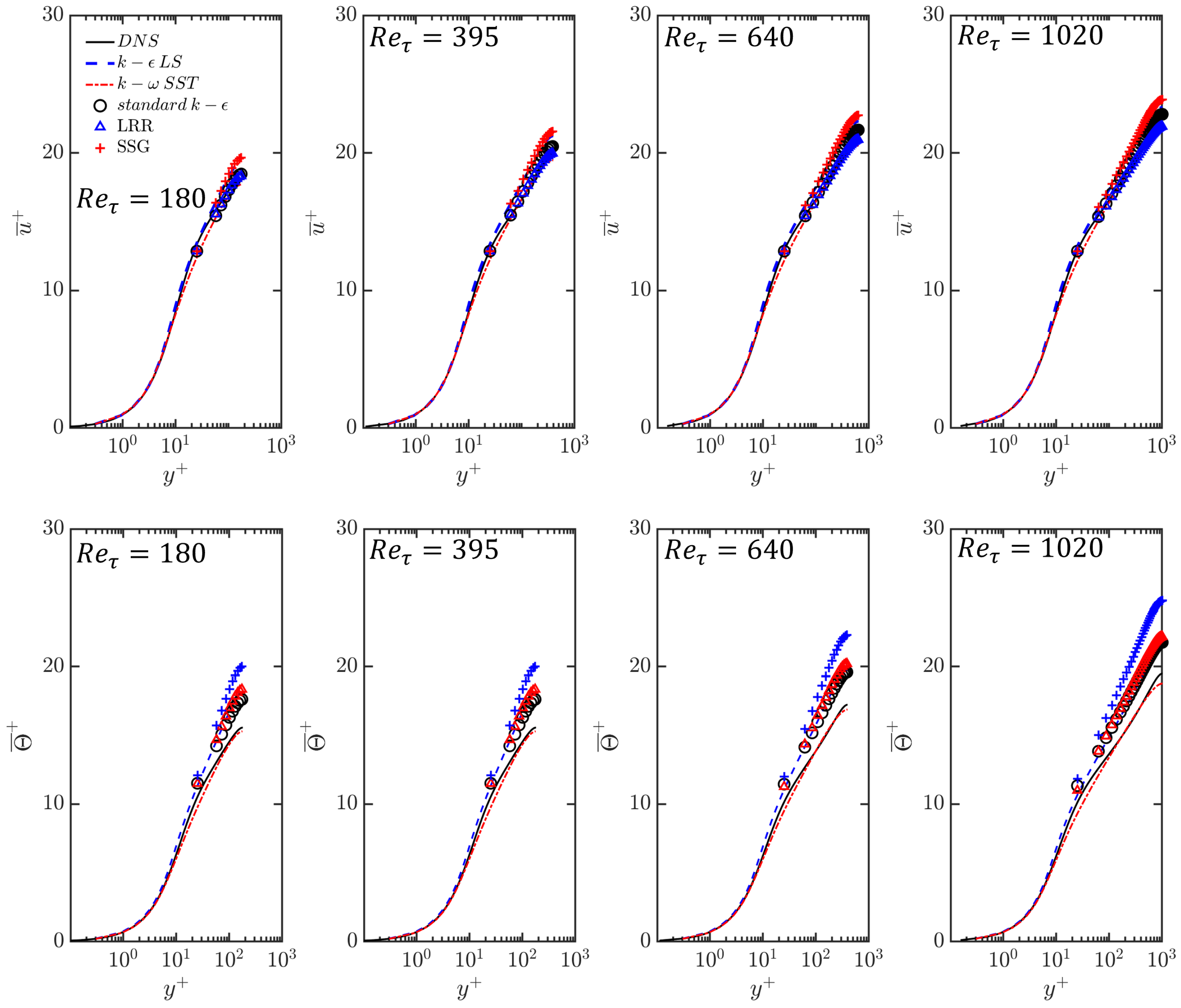
The velocity statistics in this configuration are expected to exhibit self-similarity, which is independent of the Reynolds number. It has indeed been found that the mean behaviour of the streamwise velocity and temperature remains unchanged despite variations in $R{e}_{\tau }$. This can be substantiated by Figure 4, where self-similarity is demonstrated by the variations of the mean profiles of the streamwise velocity and temperature obtained from both DNS and turbulence model predictions.

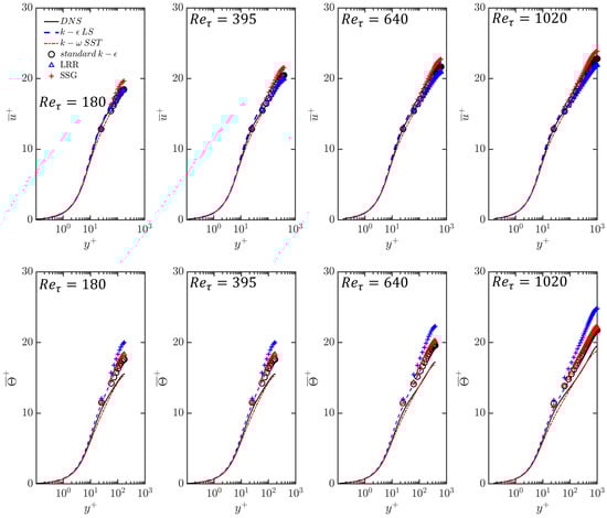
Figure 4. The velocity and temperature profiles at $Pr=0.71$ with different $R{e}_{\tau }$.

Turbulence models encounter difficulties in precisely predicting intricate fluid dynamics spanning a broad spectrum of Reynolds numbers, especially in the context of low-Reynolds-number flows undergoing transitional states. Nevertheless, these models perform well across a wide range of $R{e}_{\tau }$ values. To evaluate the qualitative performance of different turbulence models and their trends with increasing $R{e}_{\tau }$, the Root-Mean-Squared (RMS) deviation is utilised to measure the differences between the values obtained from DNS and the values predicted by the five models. Thus, the RMS of the relative deviation of the mean velocity between the DNS and RANS predictions based on the turbulence model $Error\left({\overline{u}}^{+}\right)$ and the RMS of the relative deviation of the mean temperature between the DNS and RANS results based on the turbulence model $Error\left({\overline{\mathsf{\Theta }}}^{+}\right)$ are given as follows:

$$Error({\overline{u}}^{+})=RMS\left(\frac{{\overline{u}}_{DNS}^{+}-{\overline{u}}_{RANS}^{+}}{{\overline{u}}_{DNS}^{+}}\right),$$

(9)

$$Error\left({\overline{\mathsf{\Theta }}}^{+}\right)=RMS\left(\frac{{\overline{\mathsf{\Theta }}}_{DNS}^{+}-{\overline{\mathsf{\Theta }}}_{RANS}^{+}}{{\overline{\mathsf{\Theta }}}_{DNS}^{+}}\right).$$

(10)

In the above equations, ${\overline{u}}_{DNS}^{+}$ represents the mean non-dimensional streamwise velocity obtained from DNS and ${\overline{u}}_{RANS}^{+}$ represents the mean non-dimensional streamwise velocity obtained from RANS. Similarly, ${\overline{\mathsf{\Theta }}}_{DNS}^{+}$ and ${\overline{\mathsf{\Theta }}}_{RANS}^{+}$ represent the mean non-dimensional temperatures obtained from DNS and RANS, respectively. Since the data points are available only across the log-law layer in the high-Reynolds-number turbulence models and the major discrepancy also occurs in this region, all five models are evaluated in this region. To achieve this, the DNS and low-Reynolds-number models are sampled in the region where the high-Reynolds-number turbulence models remain valid.

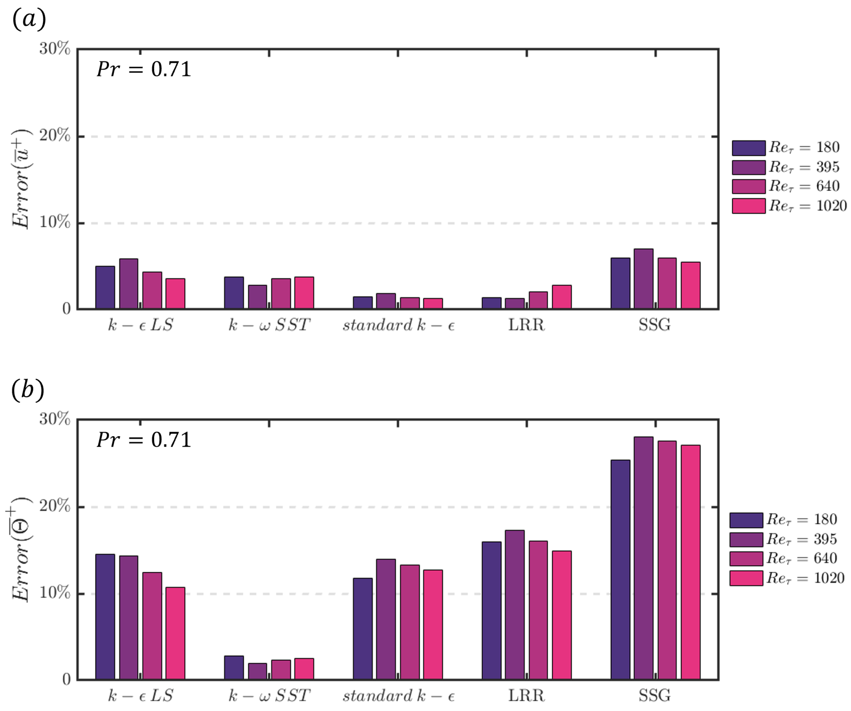
Figure 5 provides quantitative insight into how the performance of the five turbulence models varies with $R{e}_{\tau }$. All of the models performed well in predicting the mean streamwise velocity at different $R{e}_{\tau }$, with all five models having $Error\left({\overline{u}}^{+}\right)$ below $10\%$ at all Reynolds numbers. Among these models, the standard $k-ϵ$ model performs well in predicting the mean streamwise velocity distribution, while the $k-\omega SST$ model performs best in predicting the mean temperature distribution. However, except for $k-\omega SST$, significant errors are obtained in the prediction of the mean temperature, with $Error({\overline{\mathsf{\Theta }}}^{+})$ becoming larger than $10\%$ for the $k-ϵLS$, standard $k-ϵ$, and $LRR$ models, with the error of the $SSG$ model being larger than $20\%$. The discrepancy between the temperature profiles predicted by the turbulence models and those obtained from DNS can also be seen in Figure 4, where a visible gap exists between DNS and the different turbulence models, except for the $k-\omega SST$ model prediction.

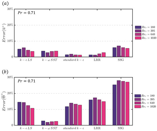
Figure 5. Error estimation of mean velocity (a) and temperature (b) of different turbulence models at $Pr=0.71$ with different $R{e}_{\tau }$.

4.1.2. Reynolds Stress Prediction

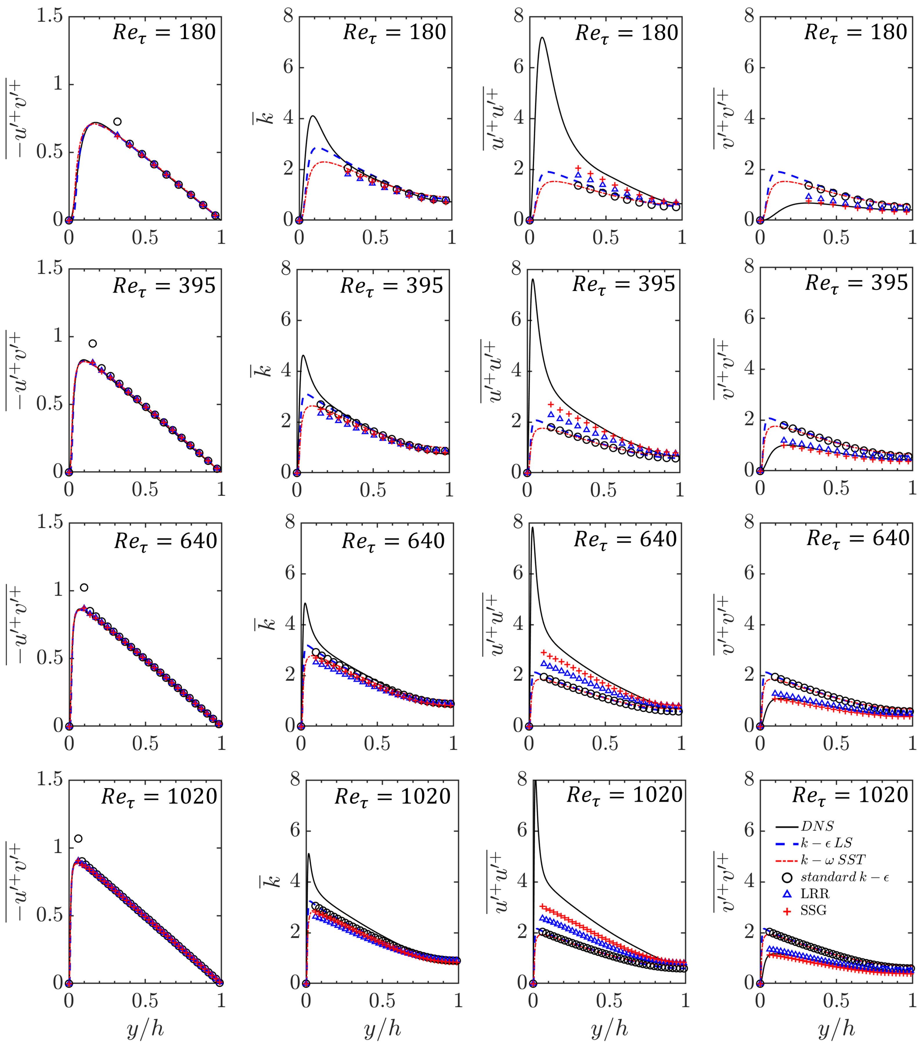
The normalised Reynolds stresses also exhibited self-similar behaviour for the range of $R{e}_{\tau }$ considered here. As shown in Figure 6, the Reynolds shear stress away from the wall collapses with different $R{e}_{\tau }$. As $R{e}_{\tau }$ increases, the peak value shifts toward the wall, while the magnitudes of the peak Reynolds shear stress remains almost the same. A similar observation can be made for the turbulent kinetic energy in Figure 6. All five models show excellent performance in predicting the Reynolds shear stress and turbulent kinetic energy, as they all align with the DNS data.

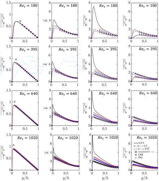
Figure 6. The profiles of the Reynolds shear stress, turbulent kinetic energy, Reynolds normal stress in the direction parallel to the wall, and normal stress in the wall-normal direction at $Pr=0.71$ with different $R{e}_{\tau }$.

However, differences can be observed in the prediction of the Reynolds normal stresses in Figure 6. The RSM closures outperform the EVM closures in this regard. The EVM models assume an isotropic distribution of eddy viscosity. In contrast, the RSM closures explicitly solve for the anisotropic Reynolds stress tensor, yielding more-accurate results in certain scenarios, such as flows with complex geometries and strong pressure gradients. Both the $LRR$ and $SSG$ modelling framework include pressure-rate-of-strain effects, but the modelling approach for the pressure–strain correlation term ${\mathsf{\Pi }}_{ij}$ is different. The $SSG$ model takes into account Reynolds stress anisotropy and non-equilibrium effects, while $LRR$ does not account for these effects. Consequently, the $SSG$ model yields a Reynolds normal stress prediction that is slightly closer to DNS compared to the $LRR$ model. However, in the current study, no major improvement in the prediction of the mean velocity and mean temperature is observed with the use of the RSM models, which is likely due to the canonical nature of the flow being studied.

4.2. Heat Transfer Rate in Turbulent Channel Flow for Different Values of Prandtl Number

4.2.1. Mean Temperature Profiles

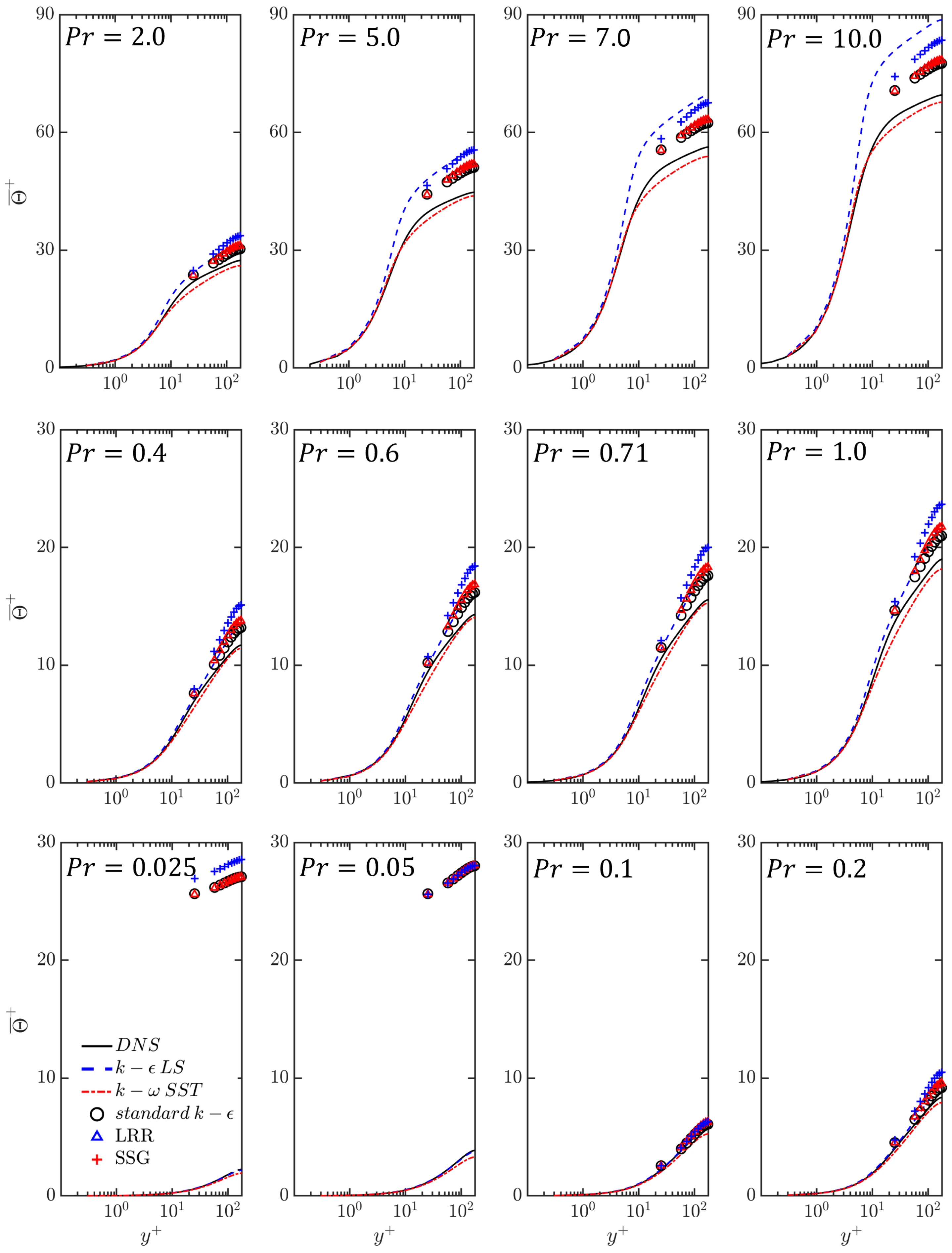
The DNS data for different values of Prandtl number are available only for $R{e}_{\tau }=180$ and $R{e}_{\tau }=395$, and thus, the RANS predictions of the mean temperature with different turbulence models are compared to the corresponding results obtained from DNS for these $R{e}_{\tau }$ values at all the Prandtl numbers available in the DNS database [1]. In Figure 7, the RANS model predictions of mean non-dimensional temperature ${\overline{\mathsf{\Theta }}}^{+}=\overline{T}/T_{\tau }$ are compared to the corresponding results extracted from the DNS data for $R{e}_{\tau }=180$ over different values of $Pr$. Both $k-ϵLS$ and $k-\omega SST$ models exhibited a similar trend as the DNS data, but $k-\omega SST$ model shows better performance, especially when the Prandtl numbers are high. However, the turbulence models with wall functions (i.e., standard $k-ϵ$, $LRR$, and $SSG$) exhibits some unexpected results in the very-low-Prandtl-number region ($Pr=0.025,0.05$), where the models significantly over-predicts ${\overline{\mathsf{\Theta }}}^{+}$. For $Pr\ge 0.1$, all the models relying on wall functions provide comparable satisfactory predictions. The temperature field exhibits distinctive characteristics across three regimes with respect to the values of the Prandtl number, which is discussed later in detail in Section 4.2.2. In the analytical regime, denoted by $Pr=0.025$ and $Pr=0.05$ for the thermal field, molecular diffusivity solely influences the thermal behaviour, which is distinctly different from the higher values of $Pr$, where both the fluid flow and temperature fields are affected by turbulent diffusion. The application of turbulence models with standard thermal wall functions is rendered ineffective in this context, as they were derived based on the assumption of eddy thermal diffusivity dominating over the molecular thermal diffusivity.

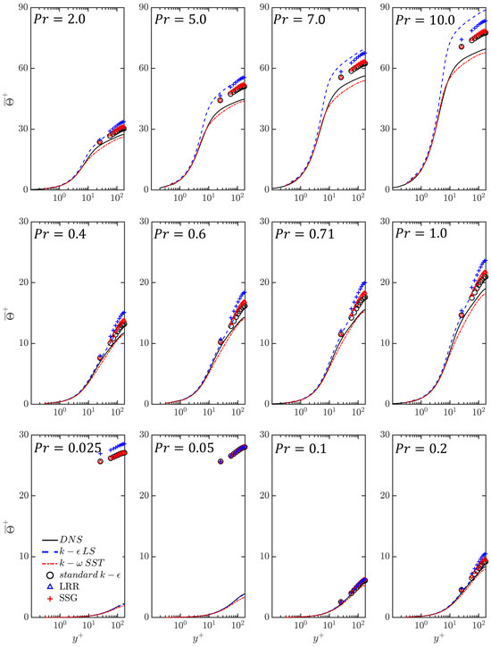
Figure 7. A comparison of mean non-dimensional temperature profiles obtained from RANS models with DNS data at $R{e}_{\tau }=180$ for different Prandtl numbers.

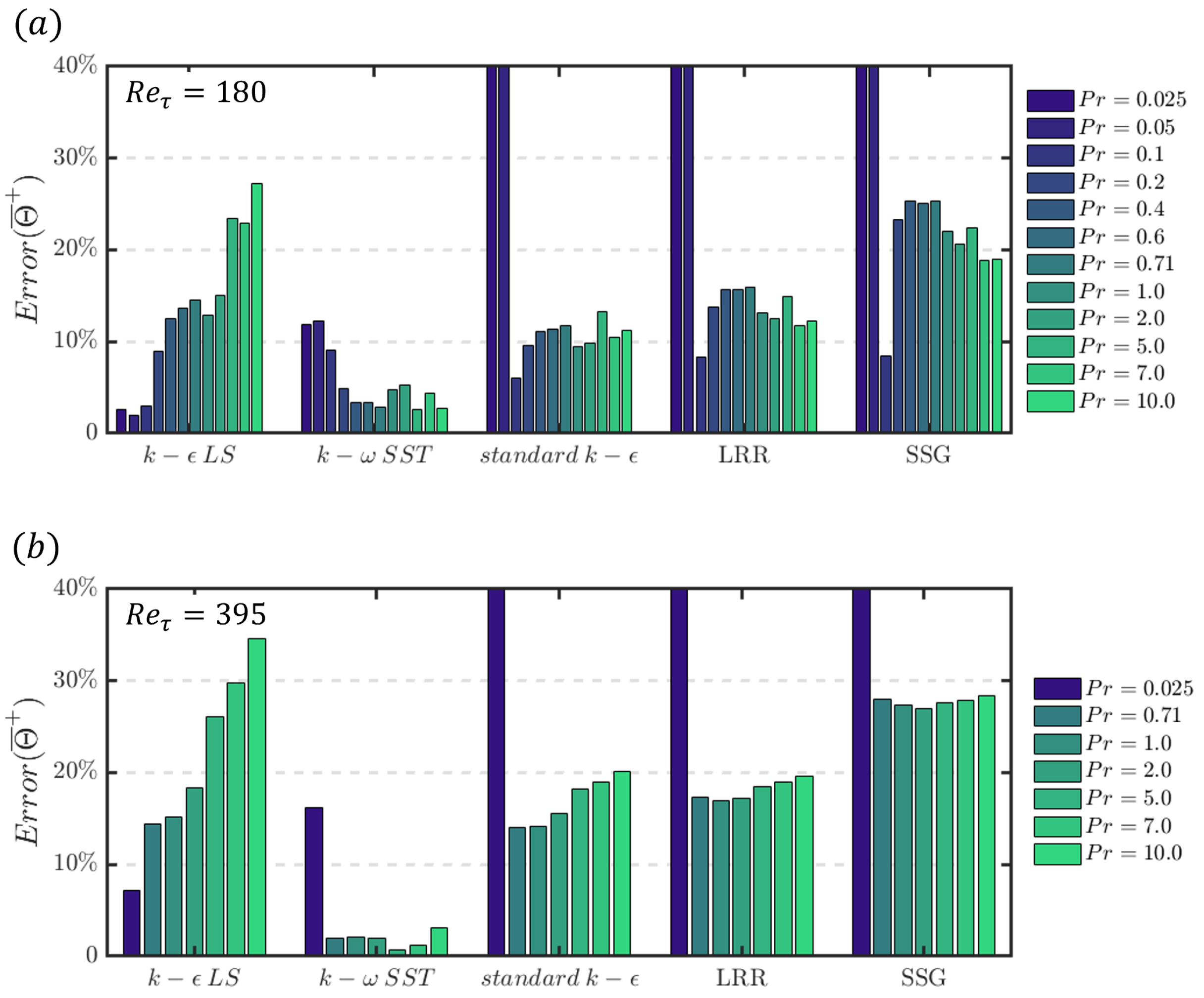
The RMS of the relative error of the mean non-dimensional temperature between DNS and turbulence model predictions for different values of $Pr$ at $R{e}_{\tau }=180$ and 395 are shown in Figure 8. The temperature profiles predicted by the standard $k-ϵ$, $LRR$, and $SSG$ models have significant errors when the Prandtl number is below $0.1$, which can also be seen in Figure 7 for $R{e}_{\tau }=180$ and $R{e}_{\tau }=395$. For Prandtl numbers greater than or equal to $0.1$, the $Error({\overline{\mathsf{\Theta }}}^{+})$ profiles of the standard $k-ϵ$, $LRR$, and $SSG$ models do not exhibit monotonicity with increasing Prandtl number. The $Error({\overline{\mathsf{\Theta }}}^{+})$ remains around $10\%$ for both the standard $k-ϵ$ and LRR models. The error of the $SSG$ model is slightly higher than that of these two models, assuming around $20\%$, and its error variation with the Prandtl number is very similar to that of the $LRR$ model.

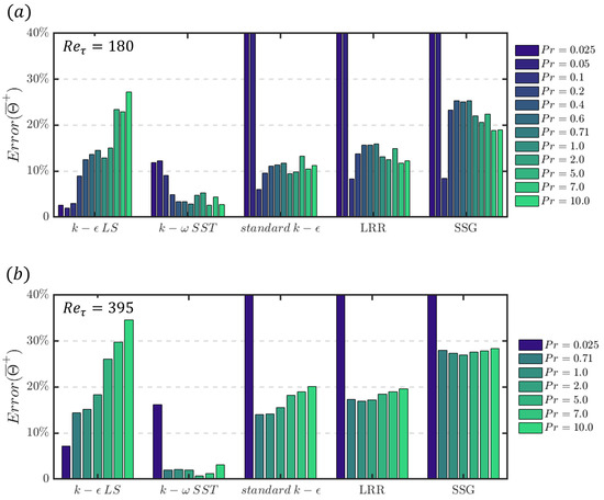
Figure 8. Error estimation of the mean temperature of different turbulence models with different $Pr$ at $R{e}_{\tau }=$ (a) 180 and (b) 395.

For models without a wall function, both the $k-ϵLS$ and $k-\omega SST$ models provides satisfactory predictions for small values of $Pr$. The $Error({\overline{\mathsf{\Theta }}}^{+})$ of the $k-ϵLS$ model for $Pr\le 0.1$ is smaller than $10\%$ at both $R{e}_{\tau }=180$ and $R{e}_{\tau }=395$. As $Pr$ increases, the $Error({\overline{\mathsf{\Theta }}}^{+})$ of the $k-ϵLS$ model gradually increases and becomes larger than $20\%$ for $Pr\ge 5$. Therefore, the $k-ϵLS$ model is more accurate when the thermal field is dominated by molecular diffusivity and becomes less accurate when the thermal field is dominated by turbulent diffusivity at both $R{e}_{\tau }=180$ and $R{e}_{\tau }=395$. On the other hand, the $k-\omega SST$ model shows the opposite trend. It is more accurate when the thermal field is dominated by turbulent diffusivity and becomes less accurate when the thermal field is dominated by molecular diffusivity. The $Error({\overline{\mathsf{\Theta }}}^{+})$ of the $k-\omega SST$ model is the smallest among all the models considered, with an error lower than $10\%$, except for very small values of $Pr$. Further analysis regarding the model performance variation with $Pr$ is provided in the following part.

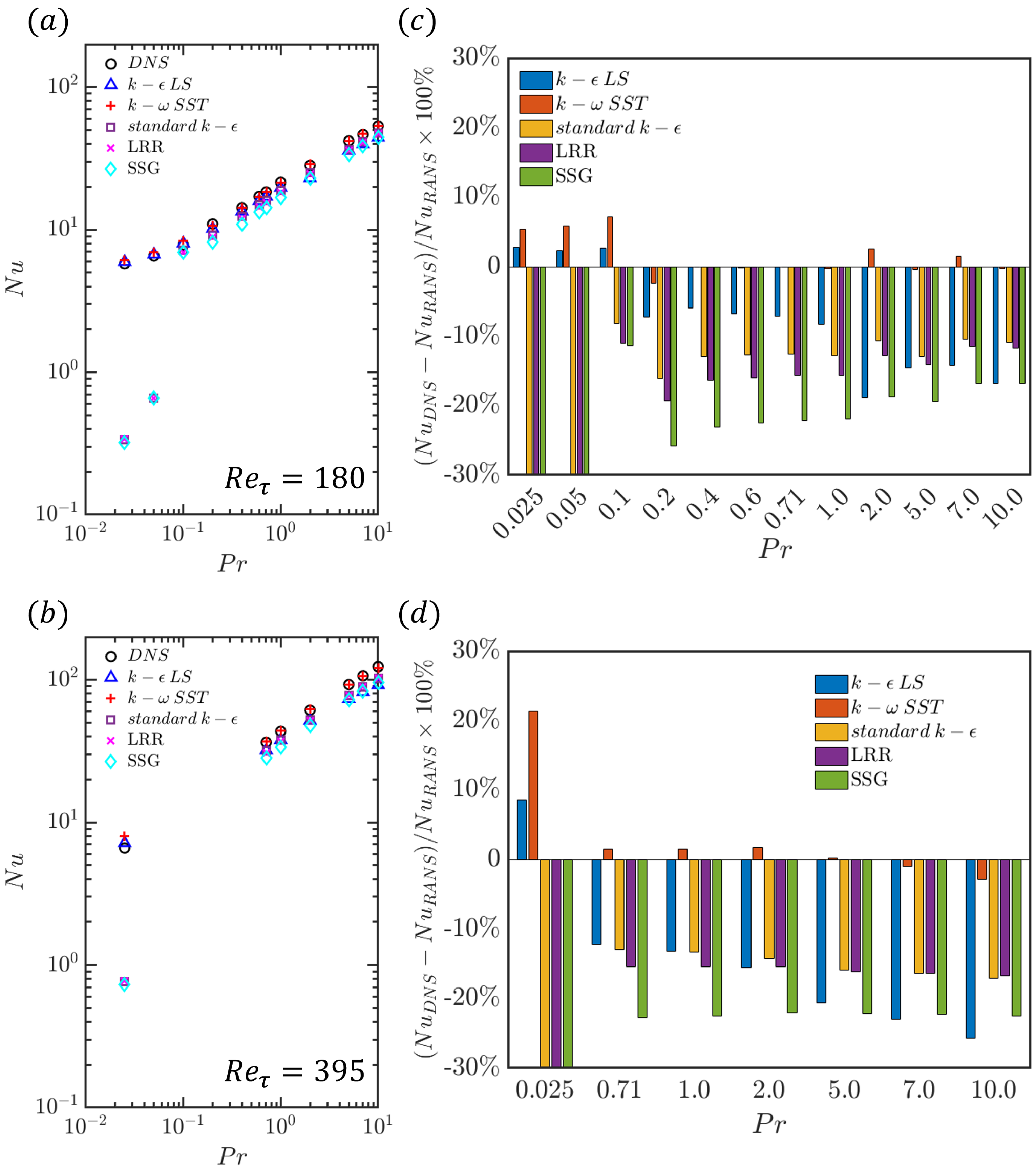
The variations of $Nu=H·h/k=\left(R{e}_{\tau }Pr\right)/({\overline{\mathsf{\Theta }}}_w^{+}-{\overline{\mathsf{\Theta }}}_b^{+})$ with $Pr$ for $R{e}_{\tau }=180$ and 395 are shown in Figure 9a,b, respectively, where H is the heat transfer coefficient, ${\overline{\mathsf{\Theta }}}_w^{+}$ is the non-dimensional temperature at the wall, and ${\overline{\mathsf{\Theta }}}_b^{+}={\int }_0^{2h}u\left(y\right)T\left(y\right)dy/\left[T_{\tau }{\int }_0^{2h}u\left(y\right)dy\right]$ is the non-dimensional bulk temperature. The Nusselt numbers obtained from different turbulence models are also compared to the $Nu$ values obtained from DNS data in Figure 9a,b. It can be seen from Figure 9a,b that all the models that rely on velocity wall functions (e.g., standard $k-ϵ$, $LRR$, and SSG models) significantly underpredict the Nusselt number for $Pr<0.1$, but all the turbulence models provide comparable predictions of $Nu$, which are of the correct order of magnitude in comparison to the DNS results. The percentage deviations of the $Nu$ predictions of the RANS models with respect to the DNS results (i.e., $(N{u}_{RANS}-N{u}_{DNS})/N{u}_{DNS}\times 100\%$) are shown in Figure 9c,d for $R{e}_{\tau }=180$ and 395, respectively. It can be seen from Figure 9c,d that the $k-ϵLS$ and $k-\omega SST$ models overpredict $Nu$ for $Pr=0.025$, $0.05$, and $0.1$, whereas all other models considered here significantly underpredict $Nu$ for these Prandtl numbers. For $Pr>0.1$, the extent of the underpredictions of $Nu$ by the standard $k-ϵ$, $LRR$, and $SSG$ models do not exhibit a monotonic trend with increasing $Pr$. The $k-ϵLS$ model shows significant underpredictions of $Nu$ for $Pr>0.1$, and this tendency strengthens with the increasing Prandtl number. The Nusselt number prediction by the $k-\omega SST$ model remains within $\pm 5\%$ of the DNS results for $Pr>0.1$, which is consistent with the fact that the $k-\omega SST$ model provides satisfactory predictions of the mean streamwise velocity and temperature distributions (see Figure 5 and Figure 8).

Figure 9. Variation of $Nu$ with $Pr$ for $R{e}_{\tau }$ = (a) 180 and (b) 395. The percentage deviations of $Nu$ predictions of RANS models with respect to DNS results (i.e., $(N{u}_{RANS}-N{u}_{DNS})/N{u}_{DNS}\times 100\%$) for different values of $Pr$ for $R{e}_{\tau }$ = (a) 180 and (b) 395.

4.2.2. Different Regimes Based on the Ratio of Eddy Thermal Diffusivity to Molecular Thermal Diffusivity

The thermal field in a fully developed channel flow experiences a transition from molecular diffusivity dominance to turbulent diffusivity dominance as the Prandtl number increases from $0.025$ to $10.0$. Different types of thermal boundary layers are obtained during this transition, which can impact the temperature distribution and heat transfer rate within the channel. Consequently, the performance of models used to describe these flows is also influenced by these characteristics.

In a fully developed thermal flow field in a channel flow configuration, there are three layers: the diffusion sublayer, intermediate layer, and log-law layer. The existence of the intermediate layer depends on the values of the Prandtl number, with $y_1^{+}$ being influenced by $Pr$, and $y_2^{+}$ depends only on $P{r}_t$ and $\kappa$, as defined in Section 3.3. With the decrease in the Prandtl number, the thermal flow field is gradually dominated by molecular diffusion effects. For extremely small values of the Prandtl numbers, the thermal field may only display molecular diffusion effects, and turbulence models with wall functions depending on the log-law may become invalid, which leads to significant errors in the prediction of the temperature fields. To validate this idea, an analytical solution is proposed. Assuming the thermal field is only influenced by molecular diffusivity, the passive scalar transport equation in a one-dimensional channel flow can be reduced as follows:

$$\frac{1}{R{e}_{\tau }Pr}\frac{d^2{\overline{\mathsf{\Theta }}}^{+}}{d{y}^{*2}}=-\frac{{\overline{u}}^{+}\left(y^{*}\right)}{⟨{\overline{u}}^{+}⟩}.$$

(11)

By integrating the Ordinary Differential Equation given above (i.e., Equation (11)), an analytical solution can be obtained. The bulk velocity, denoted by $⟨{\overline{u}}^{+}⟩$, is equal to $15.736$ at $R{e}_{\tau }=180$. While there is no analytical solution for ${\overline{u}}^{+}\left(y^{*}\right)$ in fully turbulent channel flow, approximate solutions can be obtained using polynomial fitting. This method suits different $R{e}_{\tau }$, but the velocity profiles have different polynomial expressions at different $R{e}_{\tau }$. An eighth-order spline is used to fit the mean velocity profile, resulting in the expression ${\overline{u}}^{+}\left(y^{*}\right)=-94.7y^{*8}+757.2y^{*7}-2520.5y^{*6}+4521.7y^{*5}-4733.1y^{*4}+2922.6y^{*3}-1029.4y^{*2}+194.3y^{*}$ for $R{e}_{\tau }=180$. The Pearson correlation coefficient between the velocity profile obtained from DNS and the velocity profile obtained from curve fitting is greater than $0.995$, and the RMS of the relative error between them is less than $0.5\%$. Using the polynomial approximation of ${\overline{u}}^{+}$ in Equation (11) yields the following analytical expression for ${\overline{\mathsf{\Theta }}}^{+}$ for $R{e}_{\tau }=180$:

$$\begin{array}{c}\hfill {\overline{\mathsf{\Theta }}}^{+}\left(y^{*}\right)=180Pr(-1.05y^{*10}+10.5y^{*9}-45y^{*8}+107.7y^{*7}-157.8y^{*6}\\ \hfill +146.1y^{*5}-85.8y^{*4}+32.4y^{*3}-15.8y^{*}).\end{array}$$

(12)

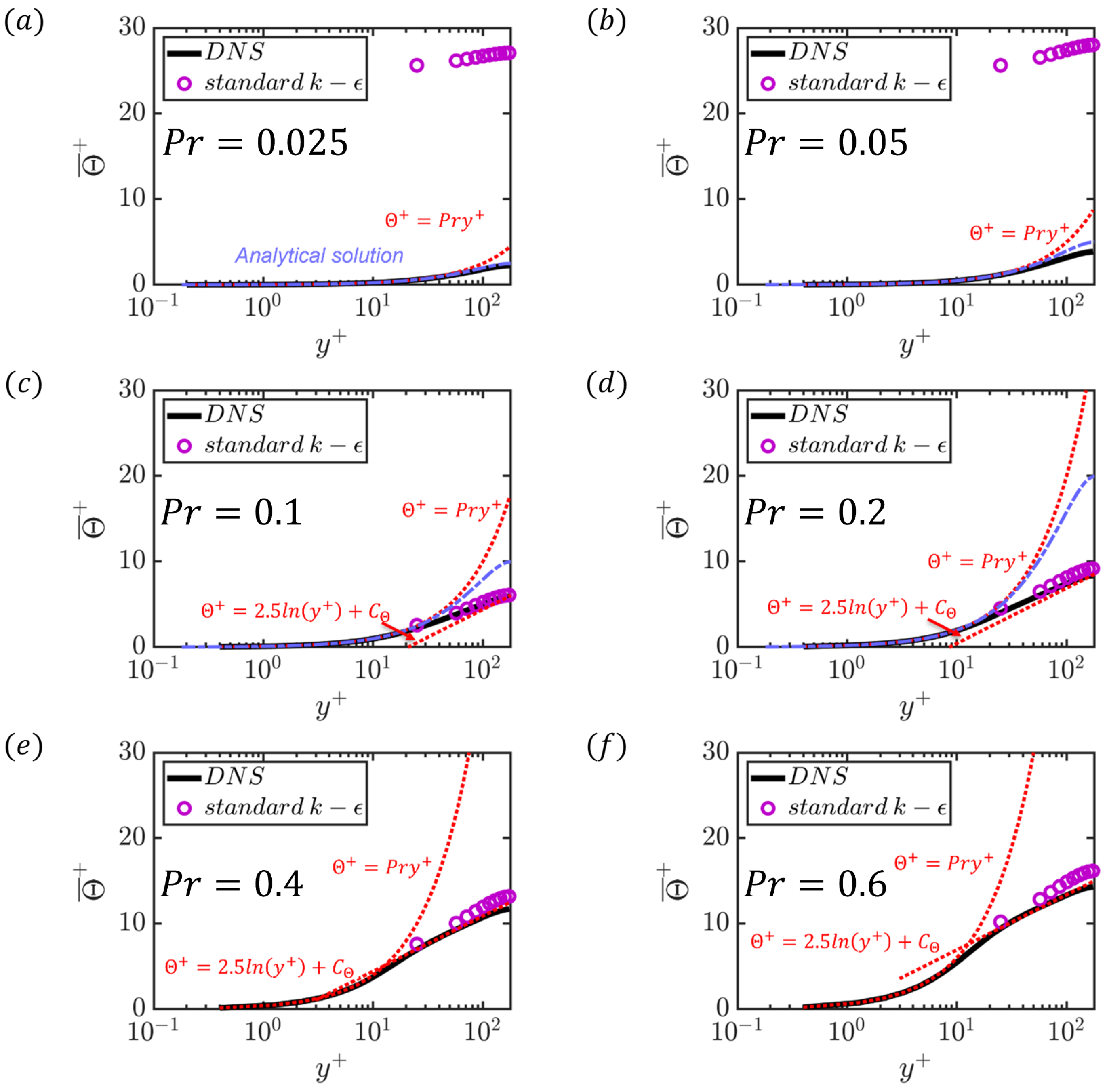
The analytical solution can be used to divide the thermal field into distinct regions based on the value of $Pr$. These regions include the analytical solution region (henceforth also called the low $Pr$ region), transitional region, and turbulent diffusivity-dominant region. Within the turbulent diffusivity-dominant region, there are two sub-regions: the $Pr\approx 1.0$ region and the high-$Pr$ (i.e., $Pr>>1$) region. The reason why these two sub-regions are defined is that the high-$Pr$ region can account for variations in the thickness of the velocity and temperature boundary layers. Table 6 provides an overview of these three regions and their corresponding $Pr$ values in the current configuration. Details along with the characteristics are discussed in Figure 10 for $R{e}_{\tau }=180$, but the same practice can be followed for other values of $R{e}_{\tau }$; however, the polynomials will be different.

Table 6. Three different regimes and the corresponding $Pr$.

Analytical Regime	Transitional Regime	Turbulent Diffusivity-Dominant Regime
		$Pr\approx 1.0$ region	high $Pr$ region
$Pr=0.025,0.05$	$Pr=0.1,0.2$	$Pr=0.4,0.6,0.71,1.0,2.0$	$Pr=5.0,7.0,10.0$

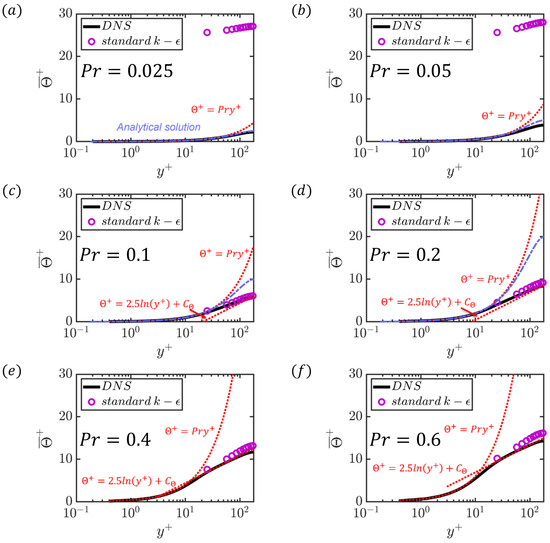
Figure 10. Three different regions in the thermal field concerning $Pr$. (a,b) are located in the analytical region; (c,d) are located in the transitional region; (e,f) are located in the turbulent diffusivity-dominant region.

In Figure 10a, the DNS result is in perfect agreement with the analytical solution, which means the thermal field is only influenced by molecular diffusivity at $Pr=0.025$. At $Pr=0.05$ in Figure 10b, the DNS result shows a slight deviation from the analytical solution, indicating that turbulent diffusivity starts to play an influential role. In this regime, the thermal field is dominated by molecular diffusivity, rendering turbulence models with wall functions depending on the log-law invalid. This low-$Pr$ regime can also be verified by using a three-layer thermal wall function and setting $y_1^{+}=y_2^{+}$. In this case, the turbulent Prandtl number is approximately equal to $0.71$, and $\kappa =0.42$. As a result, the critical Prandtl number is approximately $0.07$, and there is no existence of an intermediate layer or log-law layer when the Prandtl number is less than $0.07$.

The transitional regime can be observed at $Pr=0.1$ and $0.2$ in Figure 10c,d, respectively, where a diffusion sublayer and an intermediate layer exist. The DNS results aligned well with the analytical solution only in the diffusion sublayer, while deviations are seen in the intermediate layer, indicating that turbulent diffusivity effects became important. There is no log-law layer observed because the slope of the DNS data and the standard $k-ϵ$ model deviate from the log-law layer auxiliary line (${\overline{\mathsf{\Theta }}}^{+}=2.5ln\left(y^{+}\right)+C_{\mathsf{\Theta }}$). However, as $Pr$ increases, the mean temperature profiles of DNS and the standard $k-ϵ$ in the log-law layer gradually approached the log-law layer’s auxiliary line.

At $Pr=0.4$ and $0.6$ in Figure 10e,f, respectively, three layers can be observed in the temperature profiles: a diffusion sublayer, an intermediate layer, and a log-law layer. This behaviour is characteristic of the regime where turbulent diffusivity plays a dominant role, and the effects of turbulent diffusivity strengthen with increasing $Pr$. Additionally, the intermediate layer becomes larger as $Pr$ increases because the endpoint of the diffusion sublayer, $y_1^{+}$, decreases as $Pr$ increases, while the starting point of the log-law layer is independent of $Pr$.

5. Conclusions

In this study, five different RANS modelling strategies are assessed for their ability to predict the heat transfer rate in a fully developed channel flow across a wide range of $R{e}_{\tau }$ and $Pr$. Specifically, these modelling strategies include the standard $k-ϵ$, $k-ϵLS$, and $k-\omega SST$ models, which are all categorised as Eddy Viscosity Models (EVMs), as well as Launder–Reece–Rodi ($LRR$) and Speziale–Sarkar–Gatski ($SSG$) models, which are classified as Reynolds Stress Models (RSMs).

Firstly, the predictions of the mean velocity and thermal fields obtained from these turbulence models are compared with the corresponding quantities extracted from the DNS data. Four setups with varying friction Reynolds numbers $R{e}_{\tau }$ of 180, 395, 640, and 1020 at $Pr=0.71$ are considered to analyse the Reynolds number dependence of the model performance. The mean velocity and temperature profiles obtained from both DNS and RANS for different turbulence models are found to exhibit self-similar behaviour. The Root-Mean-Squared (RMS) deviation from the DNS data is used to quantify the difference between the turbulence model predictions and the corresponding DNS data. All models perform well in the prediction of the mean streamwise velocity, with the RMS of the relative error of the velocity $Error\left({\overline{u}}^{+}\right)$ less than $10\%$ at all values of $R{e}_{\tau }$ considered in this work. However, the performance of these models is less satisfactory for the prediction of the mean temperature, with the RMS of relative error of mean temperature $Error({\overline{\mathsf{\Theta }}}^{+})$ being larger than $10\%$ for all models, except for the $k-\omega SST$ model. Additionally, the model predictions of the second moments are also compared with the corresponding quantities obtained from the DNS data. All models perform well in the prediction of the Reynolds shear stress and turbulent kinetic energy, but the RSM closures perform better than the EVM closures in terms of the predictions of normal Reynolds stresses. Among the RSM models, the $SSG$ model outperforms the $LRR$ model due to an improved representation of the pressure strain correlation term.

Secondly, the influence of the Prandtl number on the prediction of the thermal field by different turbulence models in fully developed channel flow is considered. Nineteen setups with Prandtl numbers varying from 0.025 to 10.0 at $R{e}_{\tau }=180$ and 395 are considered. The turbulence models with the wall function are found not to predict the mean temperature and Nusselt number adequately for small values of $Pr$. However, except for the very-low-$Pr$ regime, these models performed comparably well for different choices of $Pr$. The performances of the $k-ϵLS$ and $k-\omega SST$ models show opposite trends in the prediction of the mean temperature and Nusselt number, with $k-ϵLS$ model being more accurate in the molecular diffusivity-dominated regime (i.e., small values of $Pr$) and $k-\omega SST$ model performing better in the turbulent diffusivity dominated regime (i.e., high values of $Pr$). Finally, an analytical solution is introduced to distinguish the Prandtl number dependence on thermal field predictions by the RANS models into three different regimes: the analytical regime, also called the low-Prandtl-number regime, the transitional regime, and the turbulent diffusivity-dominant regime. There are two sub-regions in the turbulent diffusivity regime: the $Pr\approx 1.0$ regime and the large-$Pr$ regime. These regimes can help understand the performance variation of a model with the variation in $Pr$.

References

- Kawamura, H.; Abe, H.; Matsuo, Y. DNS of turbulent heat transfer in channel flow with respect to Reynolds and Prandtl number effects. Int. J. Heat Fluid Flow 1999, 20, 196–207. [Google Scholar] [CrossRef]
- Johansson, A.V.; Wikström, P.M. DNS and modelling of passive scalar transport in turbulent channel flow with a focus on scalar dissipation rate modelling. Flow Turbul. Combust 2000, 63, 223–245. [Google Scholar] [CrossRef]
- Mujumdar, A.S.; Mashelkar, R.A. Advances in Transport Processes; Elsevier: Amsterdam, The Netherlands, 2013. [Google Scholar]
- Kim, J.; Moin, P. Transport of passive scalars in a turbulent channel flow. In Turbulent Shear Flows 6; Springer: Berlin/Heidelberg, Germany, 1989; pp. 85–96. [Google Scholar]
- Kasagi, N.; Tomita, Y.; Kuroda, A. Direct numerical simulation of passive scalar field in a turbulent channel flow. ASME J. Heat Transf. 1992, 114, 589–606. [Google Scholar] [CrossRef]
- Kasagi, N.; Ohtsubo, Y. Direct numerical simulation of low Prandtl number thermal field in a turbulent channel flow. In Turbulent Shear Flows 8; Springer: Berlin/Heidelberg, Germany, 1993; pp. 97–119. [Google Scholar]
- Kawamura, H.; Ohsaka, K.; Abe, H.; Yamamoto, K. DNS of turbulent heat transfer in channel flow with low to medium-high Prandtl number fluid. Int. J. Heat Fluid Flow 1998, 19, 482–491. [Google Scholar] [CrossRef]
- Abe, H.; Kawamura, H.; Matsuo, Y. Surface heat-flux fluctuations in a turbulent channel flow up to Reτ = 1020 with Pr = 0.025 and 0.71. Int. J. Heat Fluid Flow 2004, 25, 404–419. [Google Scholar] [CrossRef]
- Germano, M.; Piomelli, U.; Moin, P.; Cabot, W.H. A dynamic subgrid-scale Eddy Viscosity Model. Phys. Fluids 1991, 3, 1760–1765. [Google Scholar] [CrossRef]
- Moin, P.; Squires, K.; Cabot, W.; Lee, S. A dynamic subgrid-scale Model for compressible turbulence and scalar transport. Phys. Fluids 1991, 3, 2746–2757. [Google Scholar] [CrossRef]
- Wang, W.P.; Pletcher, R.H. On the large Eddy simulation of a turbulent channel flow with significant heat transfer. Phys. Fluids 1996, 8, 3354–3366. [Google Scholar] [CrossRef]
- Wang, L.; Dong, Y.H.; Lu, X.Y. An investigation of turbulent open channel flow with heat transfer by large Eddy simulation. Comput. Fluids 2005, 34, 23–47. [Google Scholar] [CrossRef]
- Wu, H.; Wang, J.; Tao, Z. Passive heat transfer in a turbulent channel flow simulation using large Eddy simulation based on the lattice Boltzmann method framework. Int. J. Heat Fluid Flow 2011, 32, 1111–1119. [Google Scholar] [CrossRef]
- Abe, K.; Suga, K. Towards the development of a Reynolds-Averaged algebraic turbulent scalar-flux Model. Int. J. Heat Fluid Flow 2001, 22, 19–29. [Google Scholar] [CrossRef]
- Pozorski, J.; Wacławczyk, M.; Minier, J.P. Full velocity-scalar probability density function computation of heated channel flow with wall function approach. Phys. Fluids 2003, 15, 1220–1232. [Google Scholar] [CrossRef]
- Pozorski, J.; Waclawczyk, M.; Minier, J.P. Probability density function computation of heated turbulent channel flow with the bounded Langevin Model. J. Turbul. 2003, 4, 011. [Google Scholar] [CrossRef]
- Wei, T. Heat transfer regimes in fully developed plane-channel flows. Int. J. Heat Fluid Flow 2019, 131, 140–149. [Google Scholar] [CrossRef]
- Mathur, A.; Roelofs, F.; Fiore, M.; Koloszar, L. State-of-the-art turbulent heat flux modelling for low-Prandtl flows. Nucl. Eng. Des. 2023, 406, 112241. [Google Scholar] [CrossRef]
- Mollik, T.; Roy, B.; Saha, S. Turbulence modelling of channel flow and heat transfer: A comparison with DNS data. Procedia Eng. 2017, 194, 450–456. [Google Scholar] [CrossRef]
- Alcántara-Ávila, F.; Hoyas, S.; Pérez-Quiles, M.J. DNS of thermal channel flow up to Reτ = 2000 for medium to low Prandtl numbers. Int. J. Heat Mass Transf. 2018, 127, 349–361. [Google Scholar] [CrossRef]
- Lluesma-Rodríguez, F.; Álcantara-Ávila, F.; Pérez-Quiles, M.J.; Hoyas, S. A code for simulating heat transfer in turbulent channel flow. Mathematics 2021, 9, 756. [Google Scholar] [CrossRef]
- Archambeau, F.; Méchitoua, N.; Sakiz, M. Code Saturne: A finite volume code for the computation of turbulent incompressible flows-industrial applications. Int. J. Finite Vol. 2004, 1. [Google Scholar]
- Ahmed, U.; Prosser, R. Modelling flame turbulence interaction in RANS simulation of premixed turbulent combustion. Combust. Theory Model. 2016, 20, 34–57. [Google Scholar] [CrossRef]
- Klein, T.S.; Craft, T.J.; Iacovides, H. Assessment of the performance of different classes of turbulence Models in a wide range of non-equilibrium flows. Int. J. Heat Fluid Flow 2015, 51, 229–256. [Google Scholar] [CrossRef]
- Pope, S.B. Turbulent Flows; Cambridge University Press: Cambridge, UK, 2000. [Google Scholar]
- Menter, F.R. Two-Equation Eddy Viscosity turbulence Models for engineering applications. AIAA J. 1994, 32, 1598–1605. [Google Scholar] [CrossRef]
- Speziale, C.G.; Sarkar, S.; Gatski, T.B. Modelling the pressure–strain correlation of turbulence: An invariant dynamical systems approach. J. Fluid Mech. 1991, 227, 245–272. [Google Scholar] [CrossRef]
- Launder, B.E.; Reece, G.J.; Rodi, W. Progress in the development of a Reynolds-Stress turbulence closure. J. Fluid Mech. 1975, 68, 537–566. [Google Scholar] [CrossRef]
- Rotta, J. Statistical theory of nonhomogeneous turbulence. ii. Z. Phys. 1951, 131. [Google Scholar] [CrossRef]
- Hanjalić, K.; Launder, B.E. A Reynolds Stress Model of turbulence and its application to thin shear flows. J. Fluid Mech. 1972, 52, 609–638. [Google Scholar] [CrossRef]
- von Kármán, M.A. Nachrichten von der Gesellschaft der Wissenschaften zu Göttingen. Math. Phys. Kl. 1930, 58. [Google Scholar]
- Jones, W.P.; Launder, B.E. The prediction of laminarization with a two-Equation Model of turbulence. Int. J. Heat Mass Transf. 1972, 15, 301–314. [Google Scholar] [CrossRef]
- Arpaci, V.S.; Larsen, P.S. A thick gas Model near boundaries. AIAA J. 1969, 7, 602–606. [Google Scholar] [CrossRef]
- Launder, B.E.; Sharma, B.I. Application of the energy-dissipation Model of turbulence to the calculation of flow near a spinning disc. Lett. Heat Mass Transf. 1974, 1, 131–137. [Google Scholar] [CrossRef]
Disclaimer/Publisher’s Note: The statements, opinions and data contained in all publications are solely those of the individual author(s) and contributor(s) and not of MDPI and/or the editor(s). MDPI and/or the editor(s) disclaim responsibility for any injury to people or property resulting from any ideas, methods, instructions or products referred to in the content. |
© 2024 by the authors. Licensee MDPI, Basel, Switzerland. This article is an open access article distributed under the terms and conditions of the Creative Commons Attribution (CC BY) license (https://creativecommons.org/licenses/by/4.0/).