Article

Numerical Study of the Unsteady Flow in Simplified and Realistic Iliac Bifurcation Models

1
MEtRICs, Campus de Azurém, University of Minho, 4800-058 Guimarães, Portugal
2
PIEP-Innovation in Polymer Engineering, University of Minho, 4800-058 Guimarães, Portugal
3
ALGORITMI Center, Campus de Azurém, University of Minho, 4800-058 Guimarães, Portugal
4
Centro Hospitalar de Vila Nova de Gaia, Vilar de Andorinho, 4430-502 Vila Nova de Gaia, Portugal
*
Author to whom correspondence should be addressed.
Fluids 2021, 6(8), 284; https://doi.org/10.3390/fluids6080284
Submission received: 23 June 2021 / Revised: 3 August 2021 / Accepted: 12 August 2021 / Published: 14 August 2021
(This article belongs to the Special Issue Computational Biofluid Mechanics)

Abstract

:
Cardiovascular diseases are a major cause of death and disability worldwide and they are commonly associated with the occurrence of atherosclerotic plaque deposition in the vessel walls, a process denoted as atherosclerosis. This is a chronic and progressive inflammatory disease of large-/medium-sized blood vessels that affects blood flow profiles, with the abdominal aorta and its branches being one of the locations prone to the development of this pathology, due to their curvatures and bifurcations. In this regard, the effect of flow patterns was studied and compared for both a simplified three-dimensional model of aorta bifurcation on the iliac arteries and a realistic model of iliac bifurcation, which was constructed from a computational tomography medical image. The flow patterns were analyzed in terms of velocity and wall shear stress distribution, but a special focus was given to the size and location of the recirculation zone. The simulations were performed using the Computational Fluid Dynamics software, FLUENT, taking into account the cardiac cycle profile at the infrarenal aorta. The shear stress and the velocity distribution observed for both models indicated that higher shear stress occurred along the flow divider wall (inner wall) and low shear stress occurred along the outer walls. In addition, the results demonstrated that the wall shear stress profiles were deeply affected by the transient profile of the cardiac cycle, with the deceleration phase being the most critical phase to the occurrence of backflow.

Graphical Abstract

1. Introduction

Atherosclerosis is characterized by the thickening of the arterial wall, a process in which cholesterol molecules are deposited and, consequently, cause the narrowing of the arterial lumen and inadequate blood flow to organs perfused by the affected artery [1,2,3]. Although this disease seems to be simple, it usually worsens silently over the years, leading to severe conditions, and it remains a major cause of death globally [4]. Hence, there has been a growing interest in understanding the biomechanics of its formation, detection, and treatment of atherosclerotic lesions, with computational simulations being one of the main tools applied to better understand the disease and to develop new treatments [5,6,7,8].
Over the years, this pathology has been deeply studied; however, the focus has essentially been on the carotid [9,10,11,12] and coronary arteries [13,14,15,16], since these are the most commonly affected arteries. Nevertheless, the abdominal aorta branches are also of great importance, such as the renal arteries and iliac bifurcation [5,17,18,19,20]. According to the literature, patients with atherosclerotic lesions in the iliac arteries will probably show coronary disease with varying degrees of severity [21]. Moreover, when these arteries are affected, claudication can occur, which is characterized by ischemic muscle pain or weakness brought on by exertion and promptly relieved by rest [22,23]. In the presence of this pathological condition, three scenarios can occur, namely, amputation, revascularization, or the death of the patient as a result of cardiovascular events [23]. Given the impact of this disease on human health, some investigations have been conducted [18,24,25,26,27,28], but further hemodynamic studies in these stenotic arteries are needed.
In this field of investigation, various researchers have applied idealized geometries to represent the desired disease model in simplified conditions [29,30,31]. Nevertheless, in recent decades, the field of medical imaging has been developing a set of techniques that noninvasively produce images of internal anatomical structures. The two most widely used techniques include Computational Tomography (CT) imaging and Magnetic Resonance Imaging (MRI). These imaging techniques provide helpful information with diagnostic and prognostic value and also allow the generation of computational surfaces for the development of acceptable models that mimic real conditions for the improvement of numerical studies [32,33,34].
One of the earliest studies was conducted by Taylor et al. [35]. In this study, the authors simulated the blood flow in an idealized model of the abdominal aorta under resting and exercise pulsatile flow conditions. Under resting conditions, a recirculation zone was formed along the downstream wall of the aorta immediately distal to renal branches. This study also demonstrated low values of wall shear stress (WSS) at the same location. In contrast, under moderate exercise conditions, all regions of low shear stress and high oscillatory shear index were eliminated [35]. More recently, a similar study was conducted by Mohammed and co-workers [5]. The authors studied idealized stenotic and healthy renal arteries under rest and exercise conditions. The authors observed flow recirculation zones in the proximal side during rest which reduced significantly during exercise conditions. In addition, they observed that the WSS behavior at the renal bifurcation in the distal side and in the stenosis throat, was more intense during exercise when compared with rest conditions. Another interesting study was conducted by Prince et al. [22]. The research team studied the feasibility of endovascular treatment of iliac stenosis in thirty-four patients. On the basis of the results obtained, it was verified that this method has a high technical success rate, causing the relief of claudication symptoms in the majority of patients. Sanghan et al. [36] investigated the effects of iliac stenosis on abdominal aortic aneurysm (AAA) formation in both mice and humans. Their results suggested that arterial stenosis at the time of aneurysm induction leads to faster AAA growth, indicating that moderate iliac stenosis may have upstream effects on AAA progression.
Taking into account the lack of hemodynamic studies in the iliac arteries and considering their importance, the purpose of this work is to understand flow patterns, including reverse flows, in the vicinity of the iliac bifurcation considering a pulsatile flow profile. To this end, both idealized and realistic geometries were considered aiming to evaluate if there are significant differences between the flow patterns obtained. A realistic anatomic model was constructed from a CT medical image, and the flow patterns were analyzed in terms of velocity and WSS distribution, but a special focus was given to the size and location of the recirculation zone. Aiming to achieve these goals, the geometry of the different models and the respective mesh suitable to capture the relevant fluid flow details were developed. Then, the FLUENT software package was used to perform the numerical simulations defining the appropriate settings [37].
Through this study, new insights about stenosis development in bifurcation regions and the effect of considering idealized and realistic models are provided. Moreover, numerical simulations aid in evaluating the hemodynamic variables for different hemodynamic conditions.

2. Computational Model

The development of a computational model for cardiovascular applications involves different steps. First of all, it is essential to identify the anatomic region of interest and create a computer model for that specific truncated region, which should be representative of real conditions. Then, the governing equations are solved for the entire domain allowing to extract the information about hemodynamic behavior [38].

2.1. Mathematical Equations

The CFD software used, ANSYS FLUENT, solves the three-dimensional equations for mass, Equation (1), and momentum, Equation (2), assuming conservation for each variable:
v = 0
t ( ρ v ) + ( ρ v v ) = p + ( τ ¯ ¯ )
where v is the fluid velocity vector, ρ is the density, p is the static pressure, and τ ¯ ¯ is the stress tensor. The turbulence was modelled by the k- ε model, with enhanced wall treatment, which is described by Equations (3) and (4):
t ( ρ k ) + ( ρ v k ) = [ ( μ + μ t σ k ) k x j ] + G k ρ ε
t ( ρ ε ) + ( ρ v ε ) = [ ( μ + μ t σ ε ) ε x j ] + C 1 ε ε k G k C 2 ε ρ ε 2 k
where k is the kinetic energy, ε the dissipation rate, μ the viscosity, and μ t the turbulent (or eddy) viscosity. G k represents the generation of turbulence kinetic energy due to the mean velocity gradients. C 1 ε and C 2 ε are constants, 1.44 and 1.92, respectively. σ k = 1.0 and σ ε = 1.3 are the turbulent Prandtl numbers for k and ε , respectively. The turbulent viscosity is given by Equation (5), combining k and ε as follows:
μ t = ρ C μ k 2 ε
where C μ is 0.09 .

2.2. Boundary Conditions and Fluid Flow Assumptions

The abdominal aorta is an artery of great size, and therefore, the viscosity is approximately constant, which makes it possible to consider the Newtonian model to be a good approximation of the numerical simulation. This assumption was previously assessed by Carneiro et al. [39], whose study demonstrated that the differences of fluid flow behavior for Newtonian and non-Newtonian profiles are not considered significant at the presented numerical model. Due to this assumption, the numerical simulations were carried out considering a Newtonian and incompressible fluid, for which the viscosity was assumed to be 0.0004 kg/m·s and the density 1057 kg/m3. Furthermore, the wall was modelled as rigid and the k-ε turbulent model was used with enhanced wall treatment.
The numerical simulations were performed considering an unsteady inlet velocity profile as depicted in Figure 1. Taylor and Draney [40] have quantified the blood flow at the infrarenal aorta and they described an inlet velocity profile as a function of time for the complete cardiac. On this basis, Carneiro et al. [41] approximated a curve to a sinusoidal function through a numerical method using the CoNum, a numerical application written in C++ developed at the University of Minho, in order to achieve the maximum velocity of the pulsatile waveform and define the inlet velocity value.
Thus, the pulsatile inlet velocity is defined by Equation (6), where V in m / s is obtained by multiplying the resulting value for 10 2 .
V ( t ) = 2.46 + 5.10 c o s ( 2 π t ) 1.93 c o s ( 4 π t ) 4.93 c o s ( 6 π t ) 0.919 c o s ( 8 π t ) + 5.81 s i n ( 2 π t ) + 6.72 s i n ( 4 π t ) + 0.395 s i n ( 6 π t ) 1.07 s i n ( 8 π t )
where V is the inlet velocity in the axial direction (m/s) and t is the time (s).

2.3. Numerical Solution

The numerical solution of the governing partial differential equations begins by discretizing the domain into elementary control volumes, using the commercial software package ANSYS®. Then, FLUENT software is used to solve the equations of continuity, momentum, and turbulence in each control volume, guaranteeing conservation for each variable. Each equation is integrated over each control volume and values of the dependent variable and its derivatives at control surfaces are approximated in terms of nodal values at surrounding points [42]. In summary, the differential equations are approximated by a set of algebraic equations over the computational domain and the algebraic equations are subsequently solved. The standard scheme for solving the pressure equation and the second-order upwind scheme to discretize the momentum, turbulence kinetic energy, and turbulence dissipation rate equations were used. Solutions are obtained iteratively, solving the equations sequentially, using the segregated solver with the Semi-Implicit Method for Pressure-Linked Equations (SIMPLE) algorithm for the pressure-velocity coupling. The convergence is accepted when the residuals are below 10 5 .

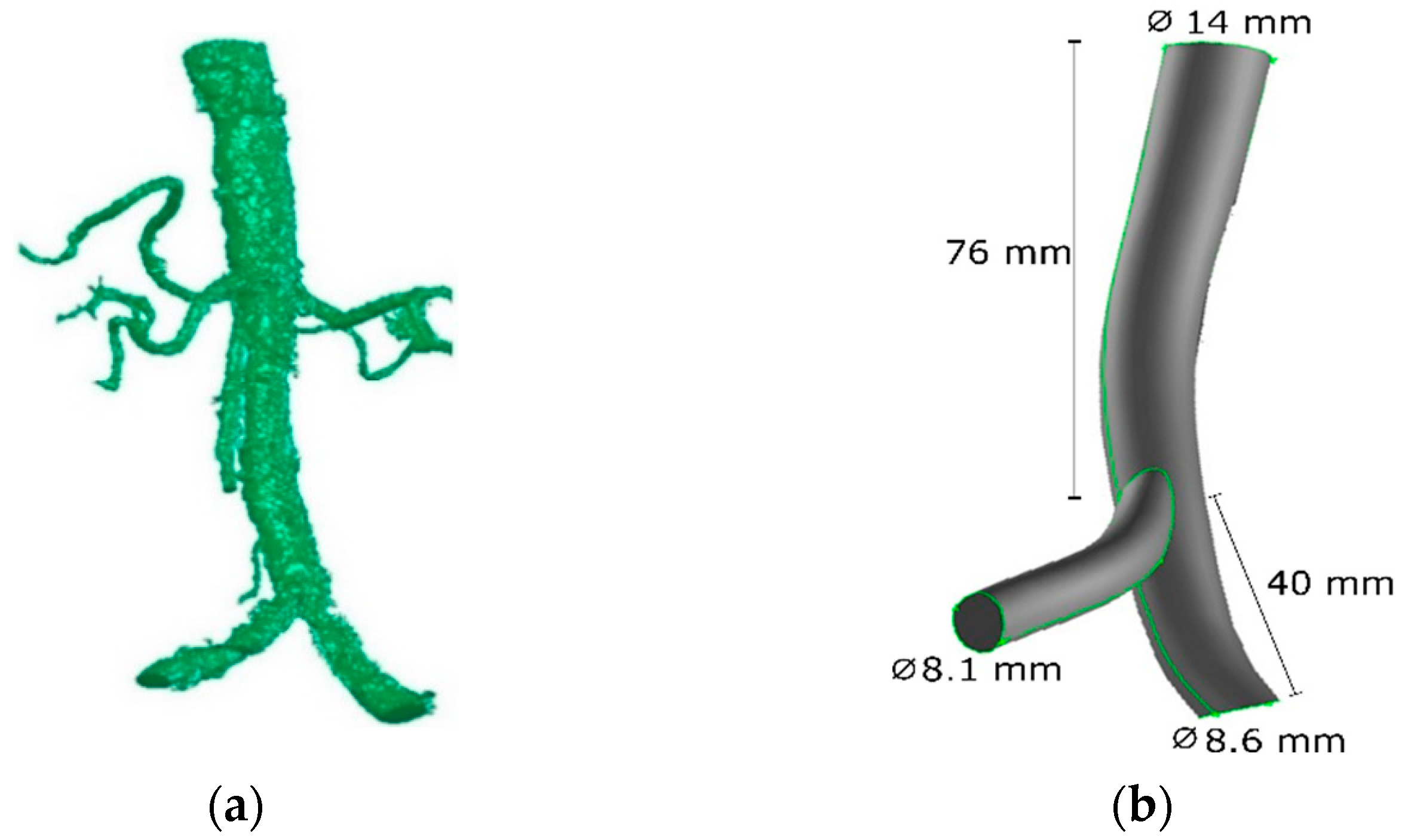
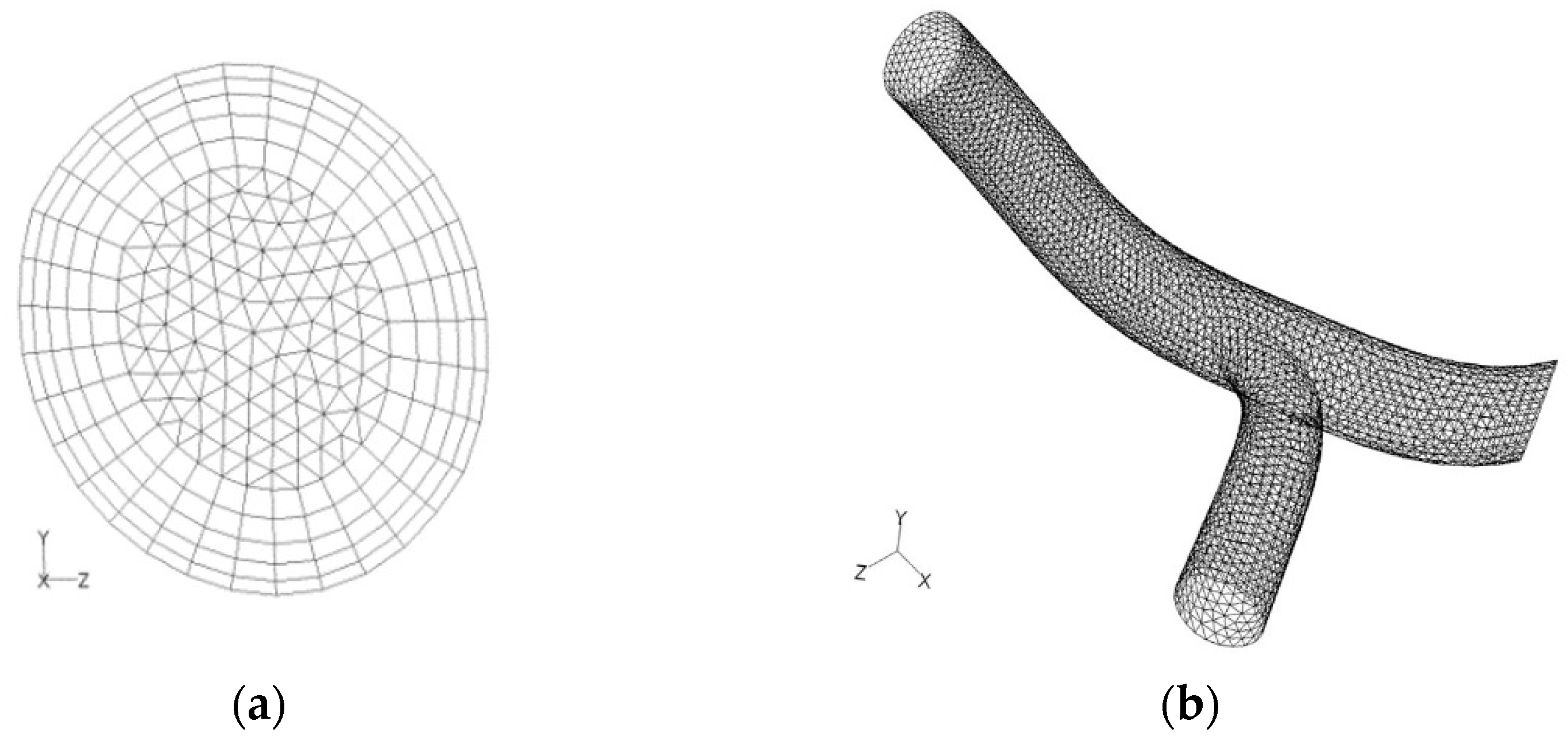
3. Geometry and Mesh

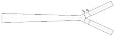
3.1. Simplified Model

A schematic representation of the three-dimensional geometry considered in this investigation and the configuration details are given in Figure 2. Please note that both iliac arteries are assumed to have the same geometric characteristics.
After the geometry was created, the computational mesh was generated. To reduce the computational time, a symmetrical geometry is assumed in the median planes y and z, reducing the domain to just one quarter. The domain was decomposed into four connected subdomains. Specifically, two of these are at the bifurcation region, to refine the mesh near the bifurcation, where higher velocity gradients are expected. The mesh consisted of hexahedral elements of different sizes: 2.3 mm for the aorta, 0.75 mm in the bifurcation zone, and 1.4 mm for the iliac. These mesh sizes were assumed from a preliminary study, published elsewhere [39]. Boundary layers, with a growth factor of 1.2, were considered at the cross-section throughout the entire domain, to refine the mesh near the walls, and at the inlet and outlet faces of the abdominal aorta. It should be referred that grid refinement tests were performed, and the following mesh showed to be adequate to perform the numerical simulations.
The resulting computational domain for this model was built with 13,376 hexahedral elements (Figure 3).

3.2. Anatomic Model

Considering that each individual has its own anatomical specificities, investigating the hemodynamic behavior on a real iliac bifurcation model is of great importance. The application of CFD analysis in realistic vessel models represents an important tool in the investigation of blood flow fields under real anatomical conditions.
Through a CT image, the generation of a computational model through real anatomic data is possible. Thus, a model of the abdominal aorta and iliac branches obtained from CT images of a normal adult subject was implemented in order to compare the computational results obtained from a realistic and a simplified anatomic geometry.
Briefly, the 3D geometry of the patient-specific model was obtained in a DICOM (Digital Imaging and Communications in Medicine) format, and it was segmented and post-processed using the MIMICS software (Materialise, Belgium). Then, when all the image processing steps had been concluded, the 3D model was exported in stereolithographic (STL) format, and imported to SolidWorks software. As the 3D model obtained directly from rendering the CT images had too many interferences in its surface, a second model was constructed in SolidWorks, using the first model as a source for dimensions, curvature, and bifurcation axes. A three-dimensional view of the realistic model obtained is shown in Figure 4.
The file was then imported into the pre-processor software. The domain was divided into 41,314 tetrahedral elements applying wall refinement criteria. The computational model and its mesh are shown in Figure 5. Five boundary layers, with a growth factor of 1.2, were considered at the cross-section throughout the entire domain in order to refine the mesh near the walls, and at the inlet and outlet faces of the abdominal aorta.
The simulations with the realistic model were performed according to the previously used boundary conditions, including the pulsatile input flow rate.

4. Results and Discussion

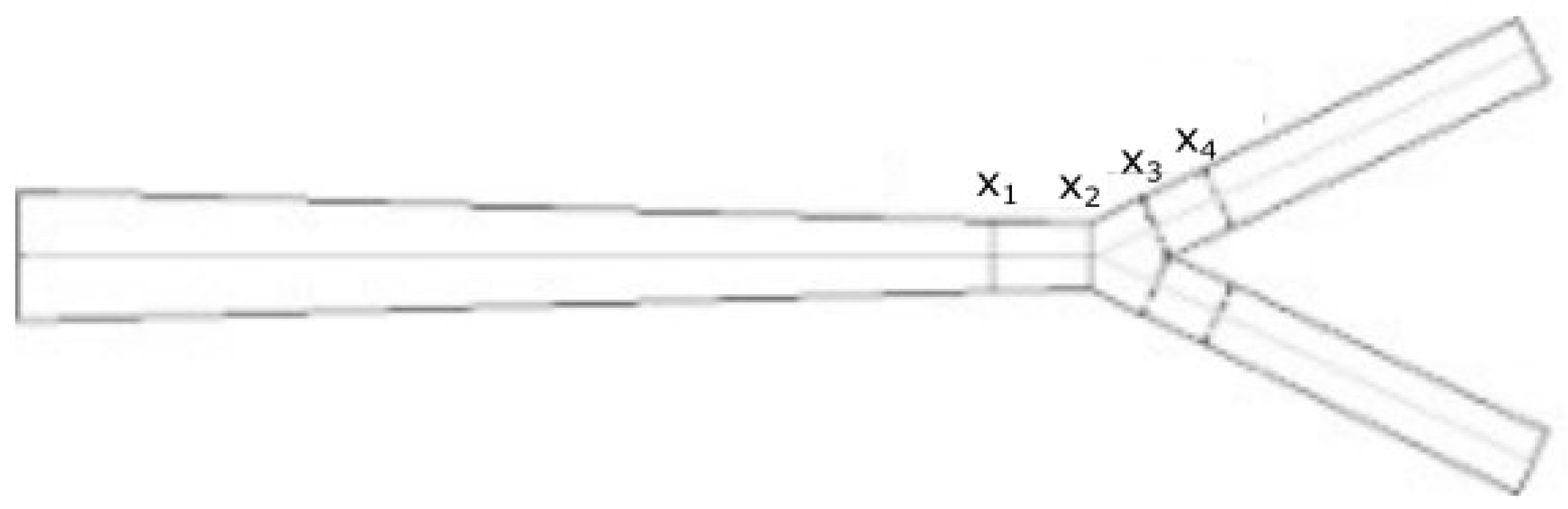
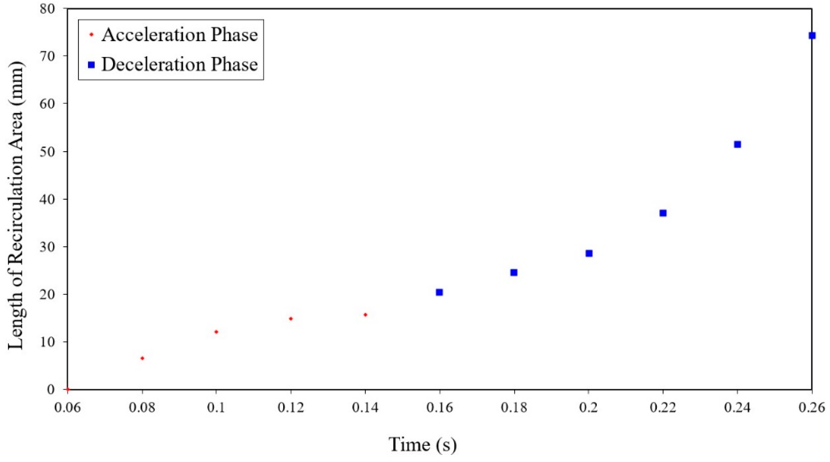
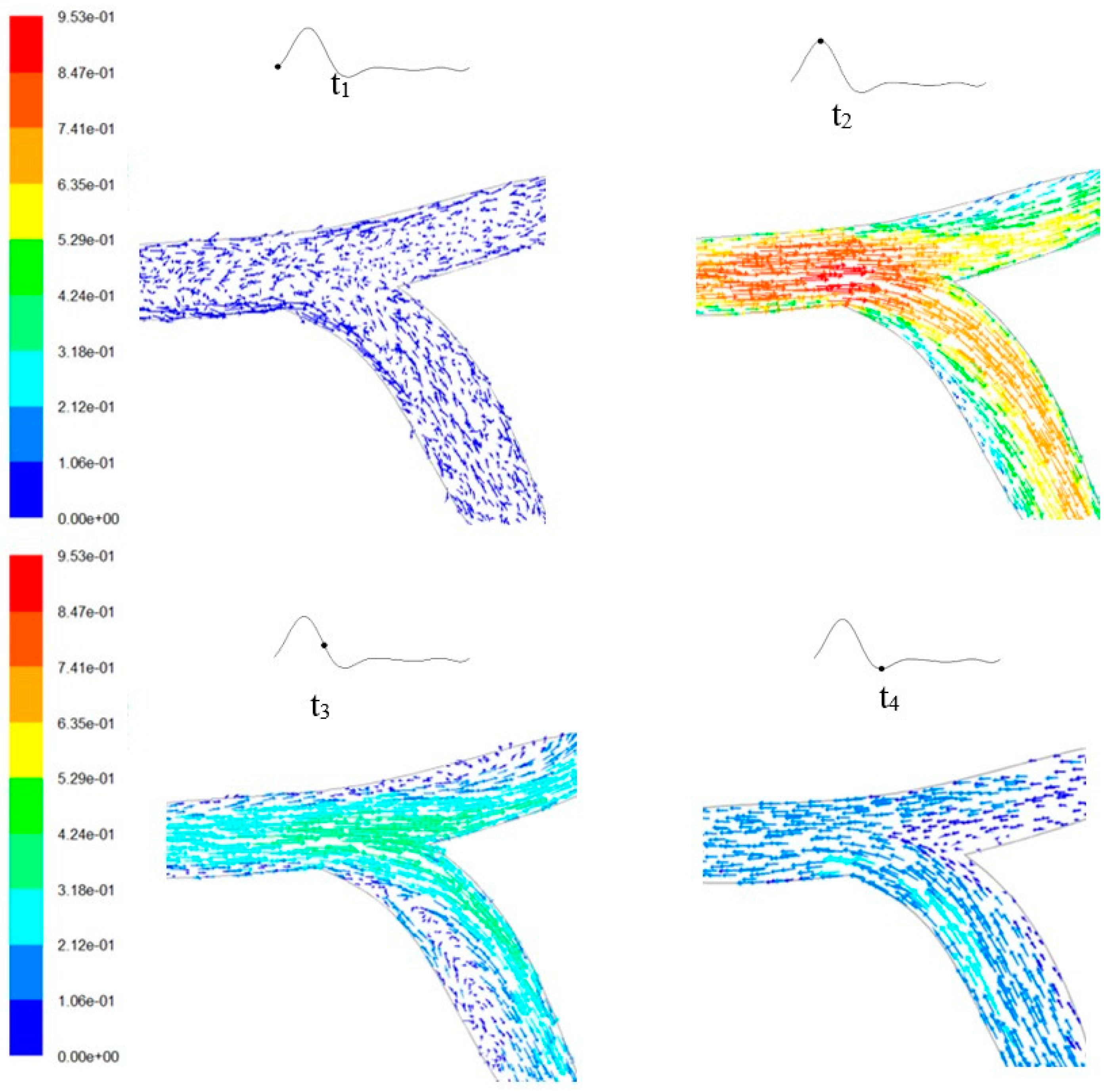
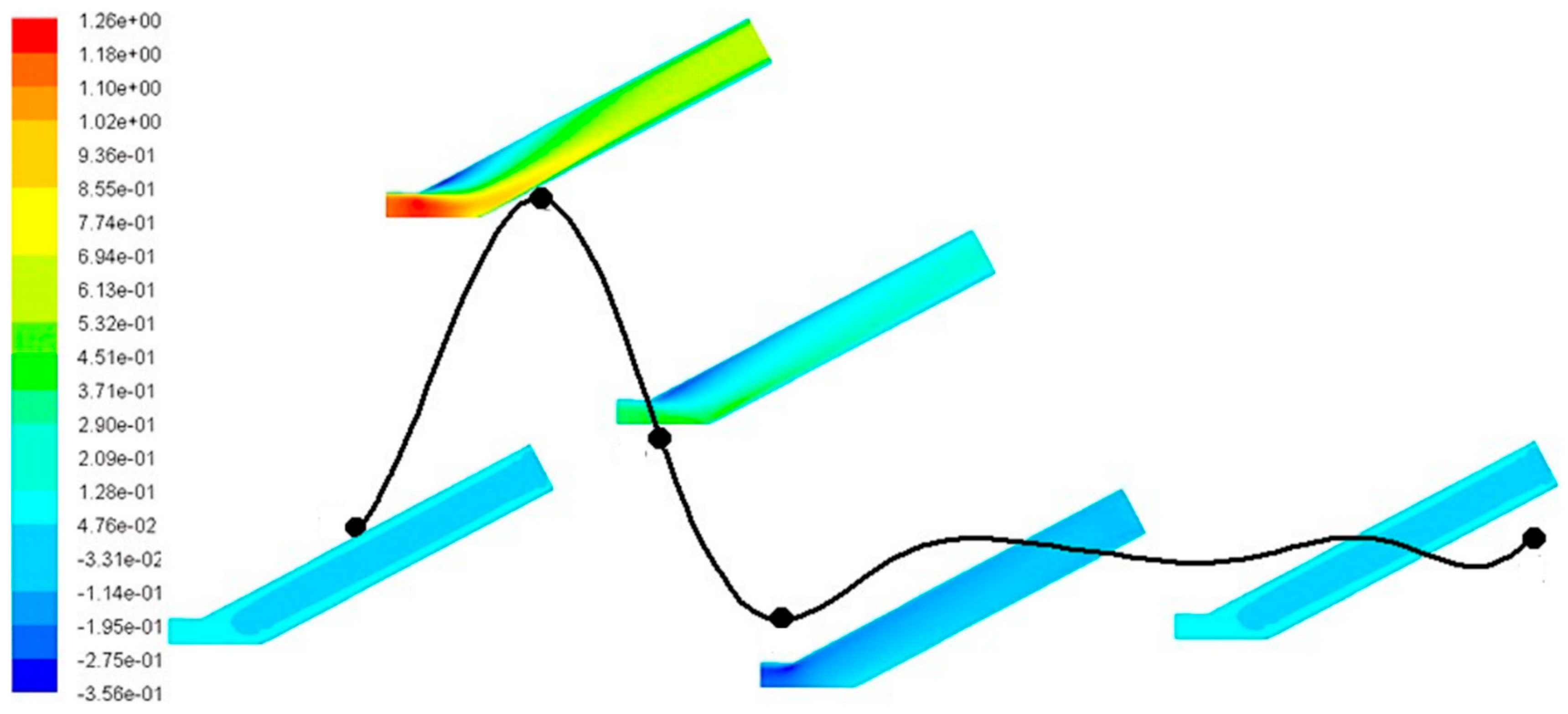
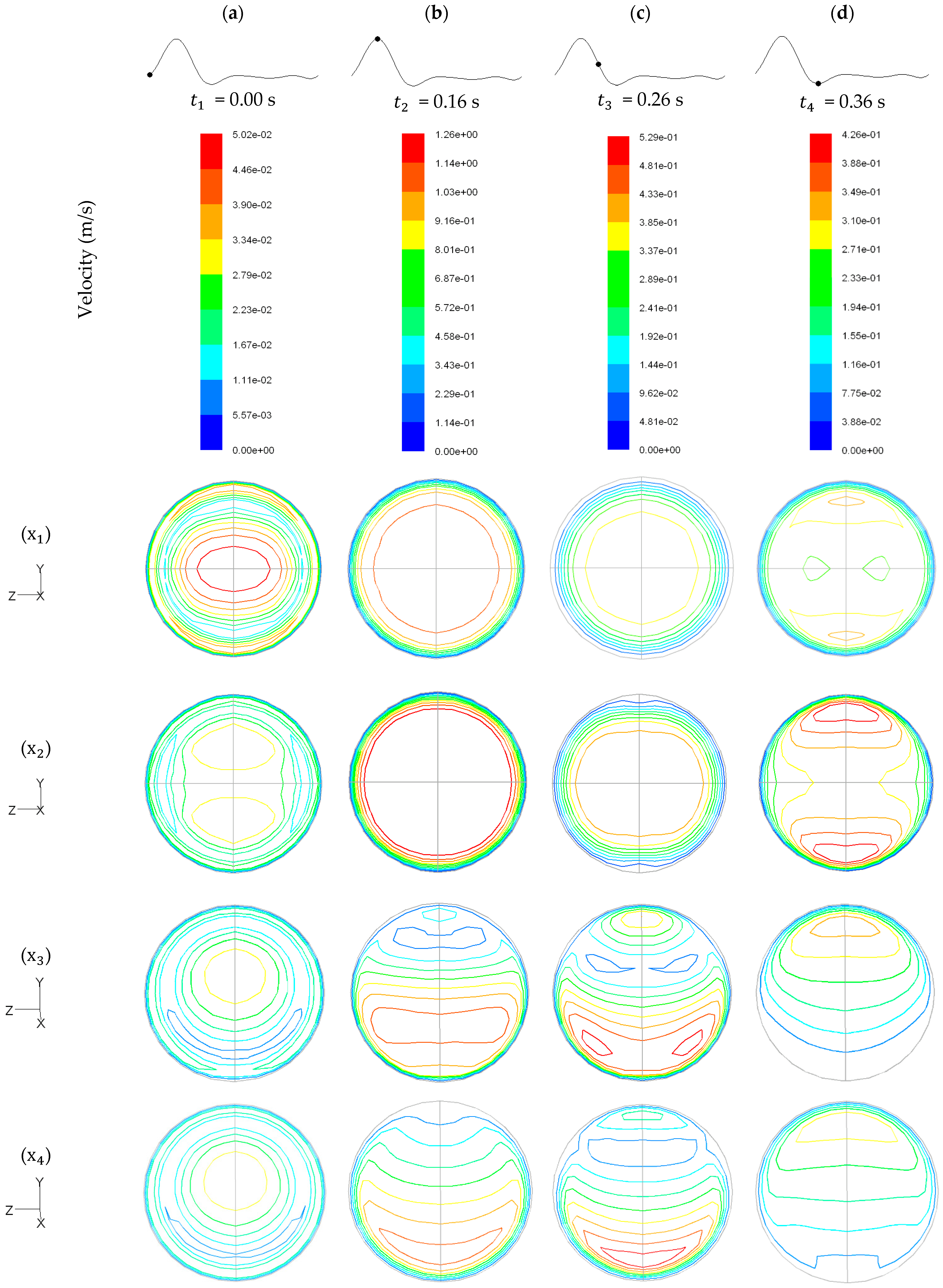
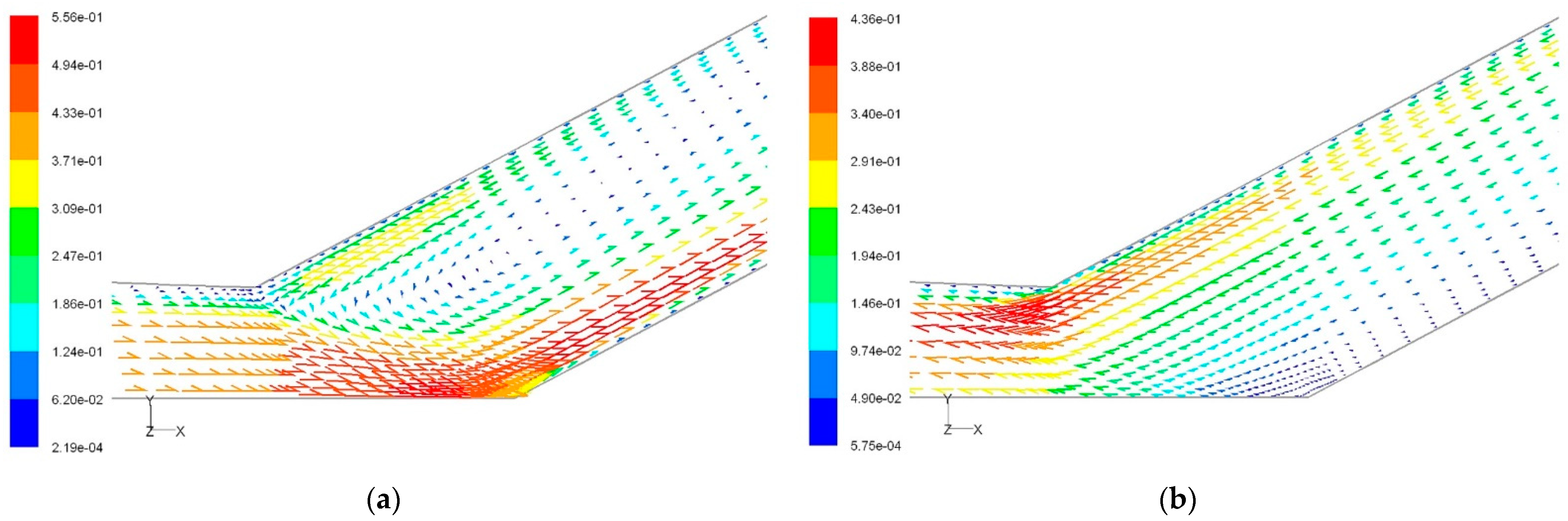
4.1. Flow in the Simplified Geometry

For the simplified geometry (presented in Figure 2), the blood flow was simulated considering the inlet velocity profile representative of the cardiac cycle infrarenal (Figure 1). The distribution of x velocities, in the vicinity of the iliac bifurcation, obtained for the time instants of t 1 = 0.00 s, t 2 = 0.16 s, t 3 = 0.26 and t 4 = 0.36 s, is shown in Figure 6.
The results show that at the beginning of the cardiac cycle ( t 1 ), the flow is not fully developed, and the velocity is positive in the whole domain, with a low value, being approximately zero. At the systolic peak ( t 2 ), the velocity increases in the central region of the abdominal aorta until the maximum value is reached, 1.26 m/s. At the instants t 2 and t 3 , the development of a recirculation region in the outer wall, downstream of the bifurcation, is also observed. At the instant t 4 , for the minimum peak, the velocity is negative in almost the entire domain.
To clarify the presentation and the discussion of the results, some regions were identified (Figure 7) in the geometry that they have received particular attention, such as, the radial lines x 1 , x 2 , x 3 , and x 4 with the axial positions of 150, 165, 175 and 185 mm, respectively.
Figure 8 presents the contours of velocity magnitude at the four transverse sections, x 1 , x 2 , x 3 , and x 4 , close to the iliac bifurcation for the different time instants of the cardiac cycle. The velocity increases at the center of the abdominal aorta, from x 1 to x 2 , the location at which the maximum velocity is found. A vortex of recirculation is formed in the position x 3 , near the outer wall of the iliac artery, decreasing to the x 4 position. In the deceleration phase, upstream of the abdominal aorta, in x 2 , two small areas of fluid recirculation close to the wall for each one of the iliac arteries are visible. Between positions x 3 and x 4 , the thickness of the vortex increases during deceleration which spreads to the entire cross-section from t 2 to t 3 instant. However, in t 4 there is a zone of positive flow on the interior wall of the iliac artery, which decreases along the axial position. In the deceleration phase for the x 3 to x 4 locations, the recirculation vortex increases both in the axial (Figure 6) and in radial directions (Figure 8), presenting this phase of the cardiac cycle is more likely to lipidic deposition.
These effects indicate that the development of atherosclerosis is, therefore, deeply correlated with the transient character of the cardiac cycle, mainly in the deceleration phase, where the recirculation expands all over the iliac artery. Figure 9 illustrates the vectors of velocity magnitude at the median plane x-y in the vicinity of the iliac bifurcation for the deceleration phase.
The formation of a vortex at the outer wall of the iliac artery for both instants of the deceleration phase is shown. From the instance t 2 to t 3 , vortex thickness increases, occupying the entire cross-section in t 3 . These observations are consistent with the results seen in Figure 8. The formation of recirculation zones close to the outer wall was also previously observed by other authors [20].
To evaluate the development of the recirculation area, the variation of recirculation spread close to the outer wall of the iliac artery during the acceleration and deceleration phases is presented in Figure 10.
Recirculation initiates at 0.06 s of the infrarenal cardiac cycle. During the acceleration phase, its increase is gradual, but in the deceleration phase, the increase of the recirculation length is more pronounced, particularly after 0.22 s. At 0.26 s, the recirculation zone reaches a value of 72 mm of length. After 0.26 s, the recirculation extends throughout the computational domain of the iliac arteries and, therefore, its length cannot be further evaluated.
The atherosclerotic plaque formation, together with its focal distribution has been associated with the variations of WSS. In fact, it has been established that arterial locations where the WSS is significantly lower in magnitude and oscillatory values occur, appear to be the highest risk areas for the increase of intimal wall thickening. The WSS distribution along the abdominal aorta and the outer and inner walls of the iliac artery is shown in Figure 11, for all representative instants of the cardiac cycle.
At the beginning of the cardiac cycle ( t 1 ), the WSS on the wall is approximately constant throughout the entire domain. The behavior of the WSS profile is similar to the deceleration phase (instants t 2 and t 3 ), but with higher values for the instant t 2 , due to higher inlet velocity. For the moment t 4 , the profile of the WSS is the opposite to that verified in the deceleration phase, except close the outer wall of the iliac artery, probably because of the negative velocity values.
The acceleration and deceleration phases of the infrarenal cardiac cycle are characterized by large fluctuations in values of WSS in the vicinity of the iliac bifurcation, associated with the formation of vortices downstream of bifurcation. The initial segment of the exterior and interior walls of the iliac arteries is the most likely site for the endothelium degradation, with subsequent deposition of plaque. Thus, atherosclerosis is more likely to be originated in the vicinity of the iliac bifurcation, because of the complex flow created by geometry features [17].

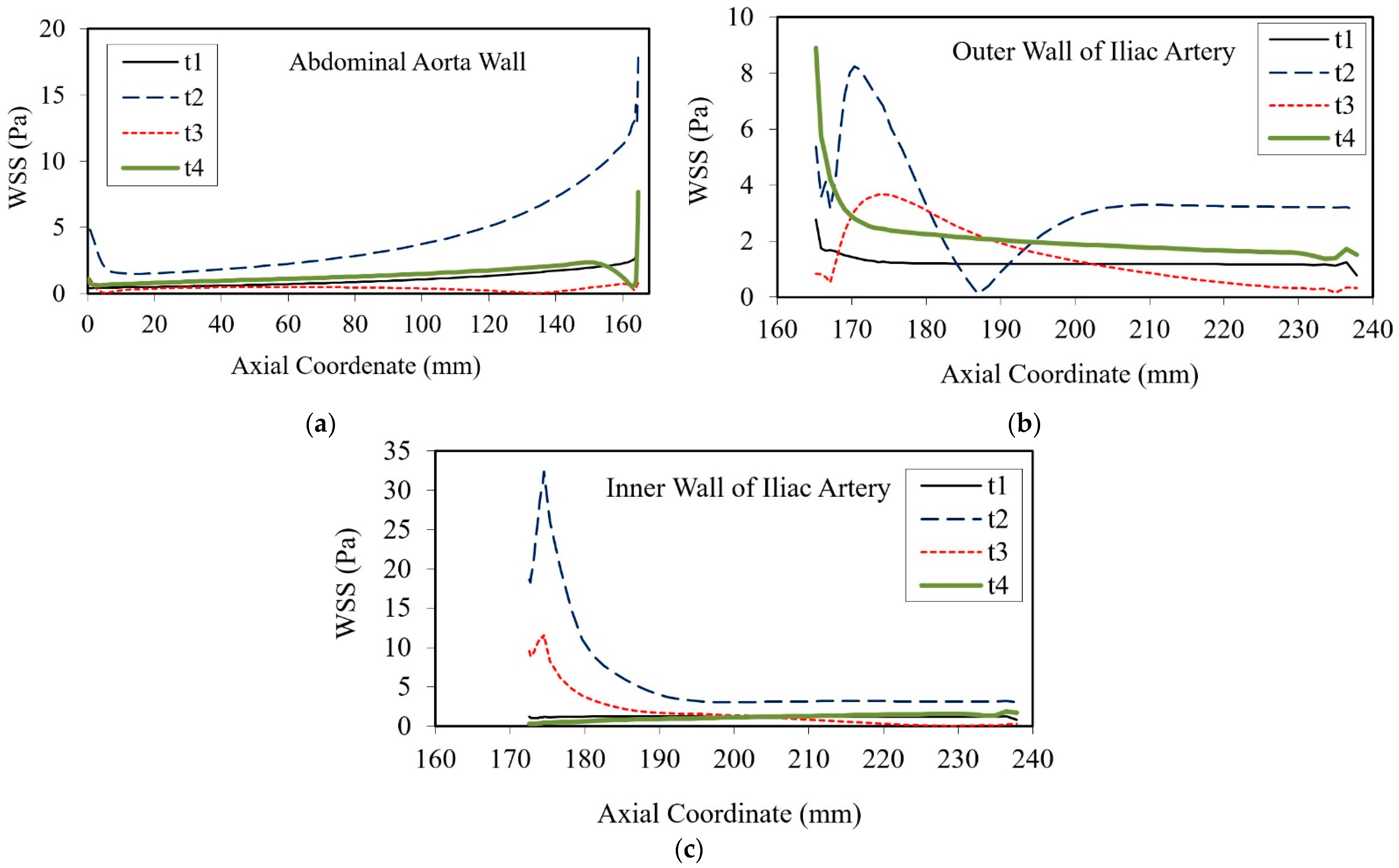
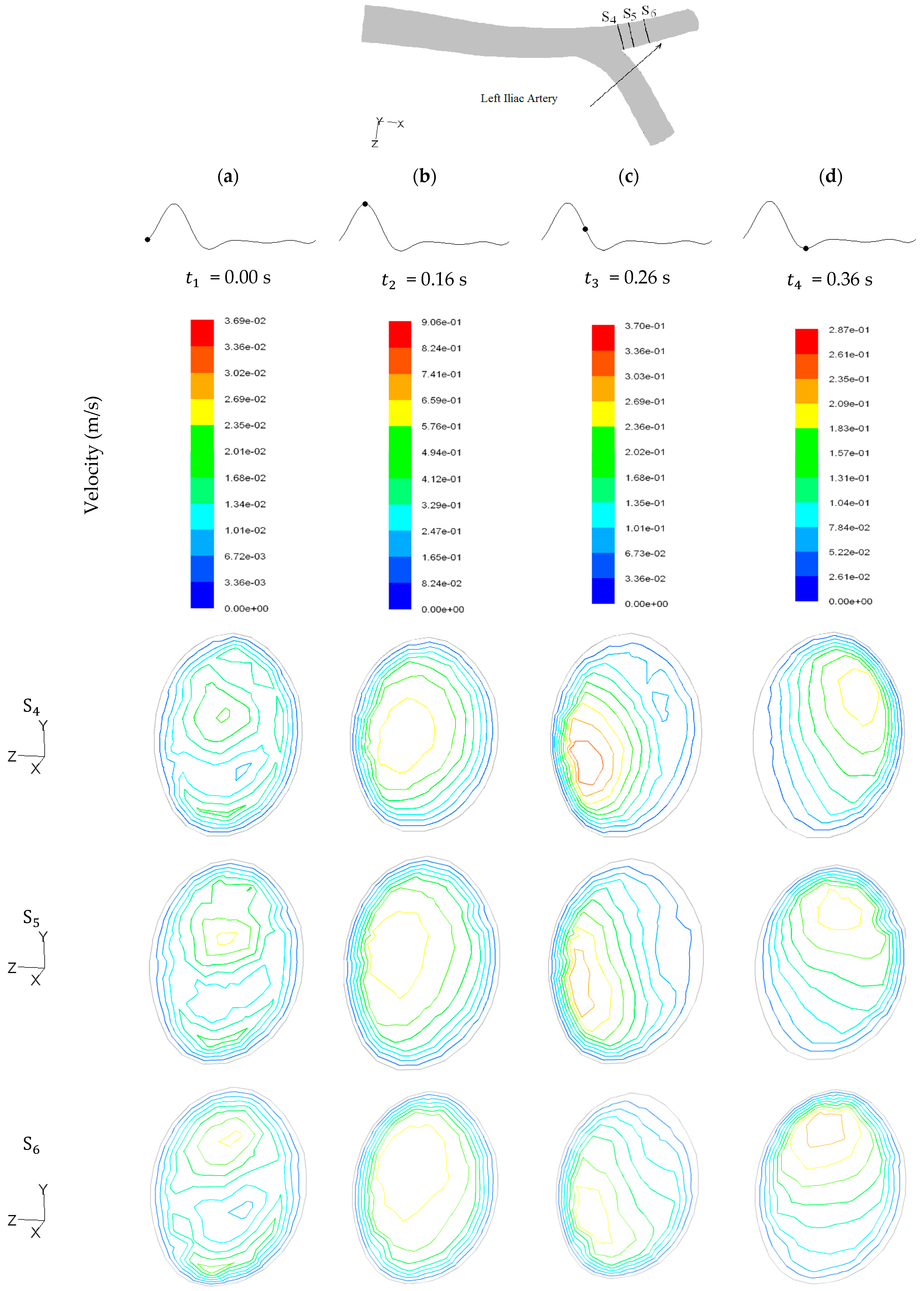
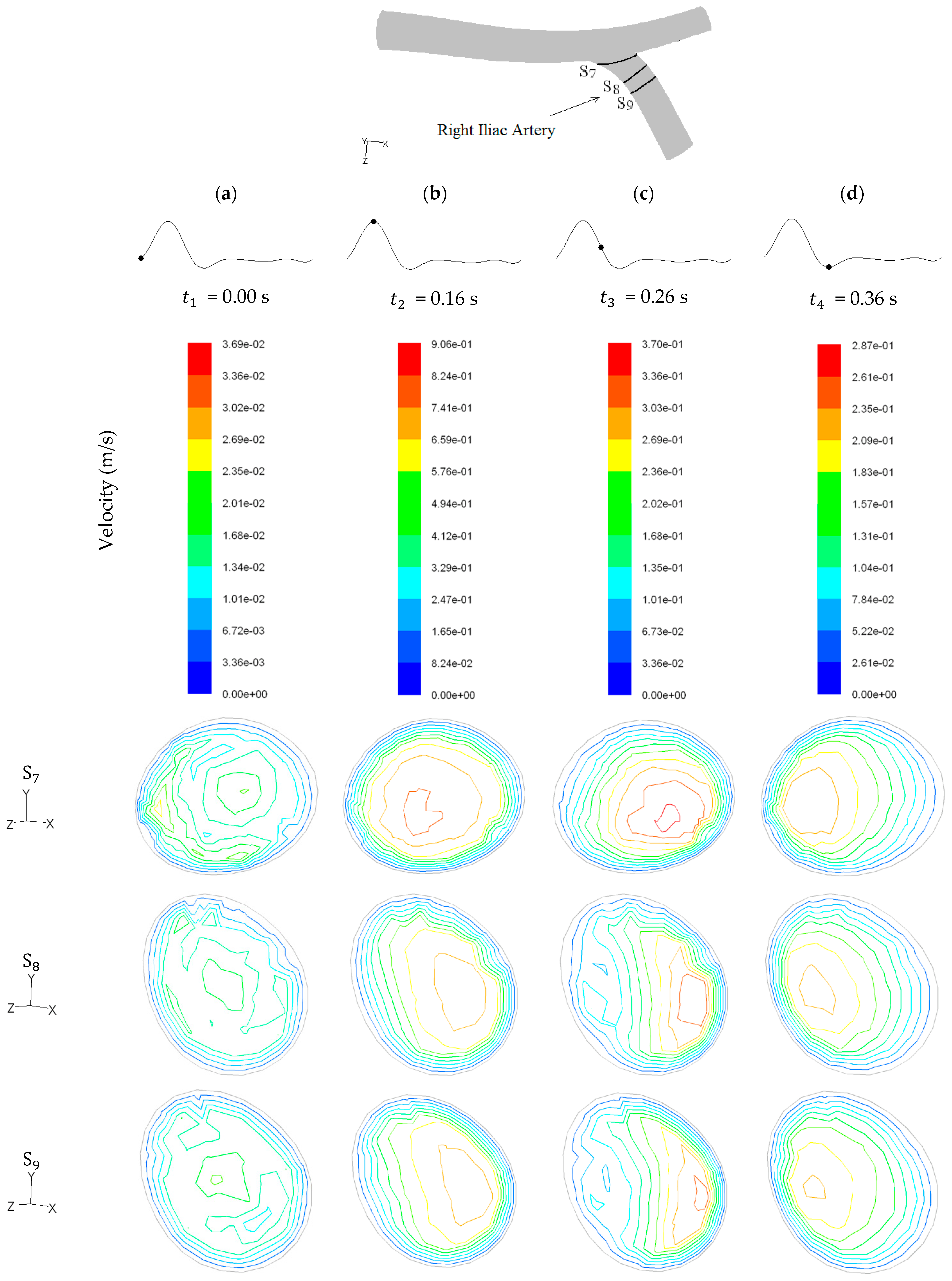
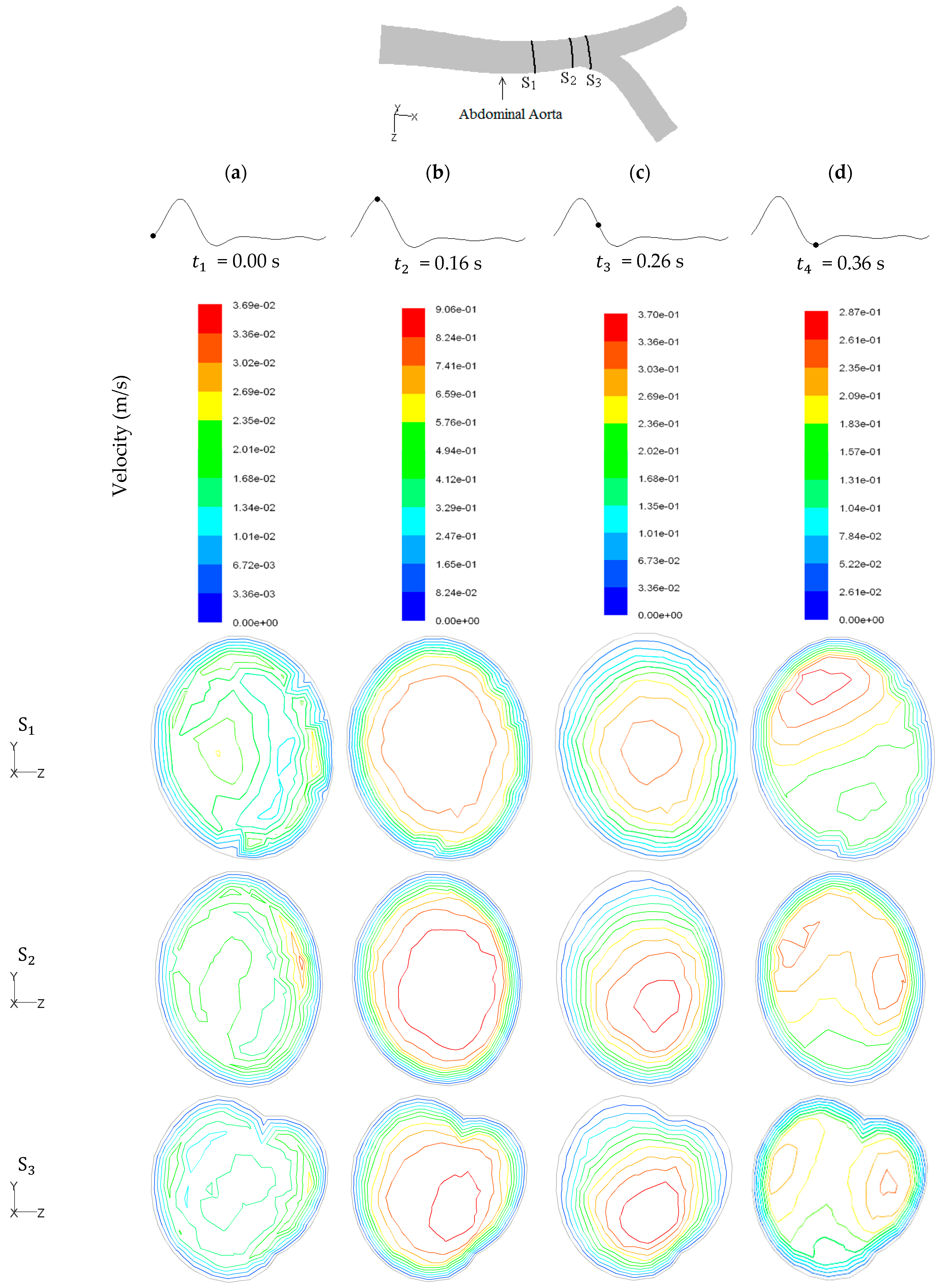
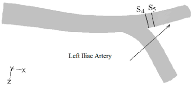
4.2. Flow in the Anatomic Geometry

Although the simplified model represents a good approximation of the realistic conditions, the assumptions and geometrical modeling present some limitations, since they do not fully describe the morphological irregularity of real arteries [32]. Therefore, the use of realistic models is crucial, as it accounts for the diameter and cross-section variations along the vessels. For this reason, in the present study, the numerical simulations of the simplified and the real iliac bifurcation geometry are compared in order to infer about the hemodynamic profiles obtained for both cases. According to this, the same study was performed for the real model along the cardiac cycle.
The vectors of velocity magnitude are presented in Figure 12 for the median x-y plane for different instants of acceleration and deceleration phase of cardiac cycle for the time instants of t 1 = 0.00 s, t 2 = 0.16 s, t 3 = 0.26 and t 4 = 0.36 s.
The division of flow between the two iliac arteries and the formation of a vortex recirculation in the outer wall of each iliac artery are visible on the basis of the analysis of the results. This vortex has larger dimensions in the right iliac artery, which may be explained through the geometry of the bifurcation. In the realistic model, there are no geometrical discontinuities close to the bifurcation, a feature that could affect the distribution of blood immediately upstream of the bifurcation. Plus, it is important to note that each artery has a different angle in relation to the positioning of the abdominal aorta, as well as the iliac arteries have different diameters. These parameters might be responsible for the non-uniform distribution of blood flow in both iliac branches. Therefore, the differences of results may be due to fact that the right iliac branch has a different shape to the left one and due to the obviously higher bifurcation angle performed by the right artery with the abdominal aorta.
The velocity profiles reveal the presence of reverse flow throughout, especially for the instants t 3 and t 4 , which correspond to the deceleration phase. It is also demonstrated that the recirculation initiates at the outer wall of iliac arteries, as happens in the simplified model, differing in the manner in which the vortex is spread. Consequently, it may be said that the deceleration of the flow is a decisive factor for the occurrence of recirculation, which is even more pronounced as the cardiac cycle evolves to the period of backflow.
The isokinetic lines for cross-sections of the abdominal aorta, right and left iliac arteries, S1–S9, for time instants of t 1 , t 2 , t 3 , and t 4 are presented in Figure 13, Figure 14 and Figure 15, respectively. The cross-sections are outlined in their respective figures. Note that the colored scales for the anatomical results were adjusted to allow the assessment of the velocity magnitude differences for each location at different instants of the cardiac cycle. Without this adjustment, the variations in the velocity would not be noticeable, especially for the instants corresponding to the deceleration phase.
Figure 13 shows that the highest velocity occurs in the center of the abdominal aorta, but in t 4 there are two peaks of velocity, suggesting the division of flow bifurcation in the two iliac arteries. Although the flow profile is more symmetrical in the first section (S1), it is verified that the maximum velocity tends to move towards the right iliac artery.
In Figure 14, the formation of a recirculation area at the outer wall of the left iliac artery is shown, during the deceleration phase ( t 3 ). In t 4 , where the vortex of recirculation t 3 was formed, the maximum velocity magnitude can be observed, suggesting that the recirculation area is extended to the entire cross-section.
Comparing Figure 13 and Figure 14, it is also demonstrated that the right iliac artery reaches higher values of velocity magnitude. The higher flow rate in this artery should be due to its higher cross-section when compared with the left iliac artery. In Figure 15, a recirculation area in cross-sections S8 and S9 can also be noted. Like the left iliac artery, it is suggested that recirculation extends to the whole cross-section.
To allow a better understanding of the results, the velocities between the two models, idealized and realistic, were compared for t 2 , which corresponds to the peak velocity of the profile shown in Figure 1. For this purpose, only the axial regions of interest were selected to perform the comparison as represented in Table 1.
Looking at the previous results, it can be observed that the velocities estimated in the anatomical model are lower than those obtained for the idealized model. This is due to the differences in the flow rates of the two models. Although the same velocity profile was used as with the idealized geometry, the actual cross-section is smaller at the inlet boundary. Nonetheless, taking into consideration the cross-section areas of the aorta and iliac arteries for both geometries, the data presented in Table 1 are in agreement with flow rate and geometric details. The differences between the right and left branches of the iliac arteries (both with diameters within 0.5 mm of each other) are due to the asymmetric flow patterns between the two branches. As can be observed from Figure 12 (at t 2 ), the higher split angle of this artery drives the main flow towards the outer wall yielding a higher peak velocity when compared with the left branch.
In summary, with this study, it was verified that although the idealized models make it possible to study the flow phenomena with a high degree of precision, the comparison between idealized geometries and the real anatomical ones cannot be carried out directly. The different curvatures of the bifurcation and possible variations in the cross-section area can result in some differences in the flow distribution, which impacts on velocity patterns, but the occurrence of recirculation vortices in the outer walls of the artery was also observed. Another conclusion is related to the specificity of the cardiac cycle, and the results show that during reverse flow, the vortex of recirculation extends to the entire section downstream of the bifurcation, as presented in Figure 15.

5. Conclusions

A simplified CFD model and a realistic one based on anatomical geometry were implemented in order to simulate the blood flow dynamics in the abdominal aorta bifurcation into the iliac arteries. The flow was modeled and the grid quality was conveniently checked. The strategy applied to the grid generation was thought to take into consideration the refinements required to capture the high variable gradients of flow patterns, and therefore, to obtain accurate results.
The shear stress distribution observed in the iliac arteries of the simplified model followed the usual trend seen in bifurcation studies with high shear stress occurring along the flow divider wall (inner wall) and low shear stress occurring along the outer walls. In addition, the WSS profiles for the simplified model were deeply affected by the transient profile of the cardiac cycle. These effects indicate that the development of atherosclerosis is, therefore, deeply correlated with the transient character of the cardiac cycle, mainly in the deceleration phase, where the recirculation expands all over the iliac artery. The velocity patterns and WSS distribution obtained in the present work are in good agreement with previous investigations [35,43].
The introduction of in vivo images in the computational models contributed to the understanding of blood flow in the descending abdominal aorta under physiologic conditions. The results of the simulation using the realistic model geometry confirmed that the more likely regions of the geometry to develop a recirculation area occur, preferentially, downstream the bifurcation at the outer walls of iliac branches.
The anatomical geometry is smoothed, reducing the geometrical discontinuities that promote the formation of atherosclerosis when compared with the simplified model. However, the simulations demonstrated that the deceleration phase of the flow is a decisive factor for the occurrence of recirculation, which is more pronounced for the period of backflow.
There are potential limitations of the presented numerical models due to the performed assumptions: the walls of the model were considered as rigid walls and the same transient inlet flow rate for both models was defined.
The pulsatile nature creates a dynamic environment that raises many interesting and fundamental unsteady fluid mechanical questions. Each feature of hemodynamics plays a role in the generation, detection, and treatment of arterial disease. This study improved our understanding that most cardiovascular diseases are highly localized and must be caused by local factors acting at a specific site of blood vessels. In conclusion, this study allowed a better understanding of the relationship between hemodynamics and vascular diseases, by assessing the distributions of blood velocity and biomechanical forces imposed on the arterial wall by the blood fluid.

Author Contributions

The authors contributed equally to the work. All authors have read and agreed to the published version of the manuscript.

Funding

This work was supported by FCT—Fundação para a Ciência e Tecnologia through the R&D Units Project Scope: UIDB/00319/2020, UIDB/04077/2020, and NORTE-01-0145-FEDER-030171, funded by COMPETE2020, NORTE 2020, PORTUGAL 2020, and FEDER.

Institutional Review Board Statement

Not applicable.

Informed Consent Statement

Not applicable.

Data Availability Statement

Not applicable.

Conflicts of Interest

The authors declare no conflict of interest.

References

  1. Libby, P.; Buring, J.E.; Badimon, L.; Hansson, G.K.; Deanfield, J.; Bittencourt, M.S.; Tokgözoğlu, L.; Lewis, E.F. Atherosclerosis. Nat. Rev. Dis. Prim. 2019, 5, 1–18. [Google Scholar] [CrossRef] [PubMed]
  2. Berger, S.A.; Jou, L. Flows in Stenotic Vessels. Annu. Rev. Fluid Mech. 2000, 32, 347–382. [Google Scholar] [CrossRef]
  3. Rogers, K. The Cardiovascular System, 1st ed.; Britannica Educational Publishing: Edinburgh, Scotland, 2011. [Google Scholar]
  4. World Health Organization (WHO). Available online: https://www.who.int/news-room/fact-sheets/detail/cardiovascular-diseases-(cvds) (accessed on 10 June 2021).
  5. Mohammed, S.; Khader, A.; Azriff, A.; Johny, C.; Pai, R.; Zuber, M. Haemodynamics behaviour in normal and stenosed renal artery using computational fluid dynamics Akademia Baru Journal of Advanced Research in Fluid Haemodynamics Behaviour in Normal and Stenosed Renal Artery using Computational Fluid Dynamics. J. Adv. Res. Fluid Mech. Therm. Sci. 2018, 51, 80–90. [Google Scholar]
  6. Barber, T. Wall shear stress and near-wall flows in the stenosed femoral artery. Comput. Methods Biomech. Biomed. Engin. 2017, 20, 1048–1055. [Google Scholar] [CrossRef] [PubMed]
  7. Carvalho, V.; Pinho, D.; Lima, R.A.; Teixeira, J.C.; Teixeira, S. Blood Flow Modeling in Coronary Arteries: A Review. Fluids 2021, 6, 53. [Google Scholar] [CrossRef]
  8. Carvalho, V.; Maia, I.; Souza, A.; Ribeiro, J.; Costa, P.; Puga, H.; Teixeira, S.F.C.F.; Lima, R.A. In vitro stenotic arteries to perform blood analogues flow visualizations and measurements: A Review. Open Biomed. Eng. J. 2020, 14, 87–102. [Google Scholar] [CrossRef]
  9. Saxena, A.; Saha, V.; Ng, E.Y.K. Skin temperature maps as a measure of carotid artery stenosis. Comput. Biol. Med. 2020, 116, 103548. [Google Scholar] [CrossRef]
  10. He, S.; Liu, W.; Qu, K.; Yin, T.; Qiu, J.; Li, Y. Effects of Different Positions of Intravascular Stent Implantation in Stenosed Vessels on In-stent Restenosis: An Experimental and Numerical Simulation Study. J. Biomech. 2020, 113, 110089. [Google Scholar] [CrossRef]
  11. Lancellotti, R.M.; Vergara, C.; Valdettaro, L.; Bose, S.; Quarteroni, A. Large eddy simulations for blood dynamics in realistic stenotic carotids. Int. J. Numer. Method. Biomed. Eng. 2017, 33. [Google Scholar] [CrossRef]
  12. Dong, J.; Wong, K.; Tu, J. Hemodynamics analysis of patient-specific carotid bifurcation: A CFD model of downstream peripheral vascular impedance. Int. J. Numer. Method. Biomed. Eng. 2013, 29, 476–491. [Google Scholar] [CrossRef]
  13. Carvalho, V.; Rodrigues, N.; Ribeiro, R.; Costa, P.F.; Lima, R.A.; Teixeira, S.F.C.F. 3D Printed Biomodels for Flow Visualization in Stenotic Vessels: An Experimental and Numerical Study. Micromachines 2020, 11, 549. [Google Scholar] [CrossRef]
  14. Carvalho, V.; Rodrigues, N.; Lima, R.A.; Teixeira, S.F.C.F. Modeling blood pulsatile turbulent flow in stenotic coronary arteries. Int. J. Biol. Biomed. Eng. 2020, 14, 1998–4510. [Google Scholar]
  15. Tajeddini, F.; Nikmaneshi, M.R.; Firoozabadi, B.; Pakravan, H.A.; Ahmadi Tafti, S.H.; Afshin, H. High precision invasive FFR, low-cost invasive iFR, or non-invasive CFR?: Optimum assessment of coronary artery stenosis based on the patient-specific computational models. Int. J. Numer. Method. Biomed. Eng. 2020, 36, 3382. [Google Scholar] [CrossRef]
  16. Seo, J.; Schiavazzi, D.E.; Kahn, A.M.; Marsden, A.L. The effects of clinically-derived parametric data uncertainty in patient-specific coronary simulations with deformable walls. Int. J. Numer. Method. Biomed. Eng. 2020, 36, 3351. [Google Scholar] [CrossRef] [PubMed]
  17. Carneiro, F.; Silva, A.E.; Teixeira, S.F.C.F.; Teixeira, J.C.F.; Lobarinhas, P.A.M.; Ribeiro, V.G. The influence of renal branches on the iliac arteries blood flow. In Proceedings of the Annual Frontiers in Biomedical Devices Conference, Irvine, CA, USA, 18–20 June 2008. [Google Scholar]
  18. Mahé, G.; Kaladji, A.; Le Faucheur, A.; Jaquinandi, V. Internal Iliac Artery Stenosis: Diagnosis and How to Manage it in 2015. Front. Cardiovasc. Med. 2015, 2, 33. [Google Scholar] [CrossRef] [PubMed] [Green Version]
  19. Shipkowitz, T.; Rodgers, V.G.J.; Frazin, L.J.; Chandran, K.B. Numerical study on the effect of steady axial flow development in the human aorta on local shear stresses in abdominal aortic branches. J. Biomech. 1998, 31, 995–1007. [Google Scholar] [CrossRef]
  20. Lee, D.; Chen, J.Y. Numerical simulation of steady flow fields in a model of abdominal aorta with its peripheral branches. J. Biomech. 2002, 35, 1115–1122. [Google Scholar] [CrossRef]
  21. Haverich, A.; Boyle, E.C. Atherosclerosis Pathogenesis and Microvascular Dysfunction, 1st ed.; Springer: Berlin, Germany, 2019. [Google Scholar]
  22. Prince, J.F.; Smits, M.L.J.; van Herwaarden, J.A.; Arntz, M.J.; Vonken, E.J.P.A.; van den Bosch, M.A.A.J.; de Borst, G.J. Endovascular Treatment of Internal Iliac Artery Stenosis in Patients with Buttock Claudication. PLoS ONE 2013, 8, e73331. [Google Scholar] [CrossRef] [Green Version]
  23. Griggs, R.; Wing, E.F.G. Cecil Essentials of Medicine, 9th ed.; Elsevier: Amsterdam, The Netherlands, 2016. [Google Scholar]
  24. Chong, A.Y.; Doyle, B.J.; Jansen, S.; Ponosh, S.; Cisonni, J.; Sun, Z. Blood flow velocity prediction in aorto-iliac stent grafts using computational fluid dynamics and Taguchi method. Comput. Biol. Med. 2017, 84, 235–246. [Google Scholar] [CrossRef] [PubMed]
  25. Huml, E.L.; Davies, R.A.; Kearns, G.A.; Petersen, S.M.; Brismée, J.M. Common iliac artery occlusion presenting with back and leg pain: Case report and differential diagnosis considerations for neurogenic/vascular claudication. J. Man. Manip. Ther. 2018, 26, 249–253. [Google Scholar] [CrossRef] [Green Version]
  26. Zhou, Y.; Tong, J.; Li, X.; Li, X.; Wang, G. Numerical simulation of haemodynamics of the descending aorta in the non-diabetic and diabetic rabbits. J. Biomech. 2019, 91, 140–150. [Google Scholar] [CrossRef] [PubMed]
  27. Andayesh, M.; Shahidian, A.; Ghassemi, M. Numerical investigation of renal artery hemodynamics based on the physiological response to renal artery stenosis. Biocybern. Biomed. Eng. 2020, 40, 1458–1468. [Google Scholar] [CrossRef]
  28. Skopalik, S.; Hall Barrientos, P.; Matthews, J.; Radjenovic, A.; Mark, P.; Roditi, G.; Paul, M.C. Image-based computational fluid dynamics for estimating pressure drop and fractional flow reserve across iliac artery stenosis: A comparison with in-vivo measurements. Int. J. Numer. Method. Biomed. Eng. 2021, 15, e3427. [Google Scholar] [CrossRef]
  29. Carvalho, V.; Rodrigues, N.; Lima, R.A.; Teixeira, S. Numerical simulation of blood pulsatile flow in stenotic coronary arteries: The effect of turbulence modeling and non-Newtonian assumptions. In Proceedings of the International Conference on Applied Mathematics & Computer Science, Athens, Greece, 31 May–2 June 2020; pp. 112–116. [Google Scholar]
  30. Li, M.X.; Beech-Brandt, J.J.; John, L.R. Numerical analysis of pulsatile blood flow and vessel wall mechanics in different degrees of stenoses. J. Biomech. 2007, 40, 3715–3724. [Google Scholar] [CrossRef]
  31. Chaichana, T.; Sun, Z.; Jewkes, J. Computation of hemodynamics in the left coronary artery with variable angulations. J. Biomech. 2011, 44, 1869–1878. [Google Scholar] [CrossRef] [PubMed] [Green Version]
  32. Doutel, E.; Viriato, N.; Carneiro, J.; Campos, J.B.L.M.; Miranda, J.M. Geometrical effects in the hemodynamics of stenotic and non-stenotic left coronary arteries—numerical and in vitro approaches. Int. J. Numer. Method. Biomed. Eng. 2019, 35, 1–18. [Google Scholar] [CrossRef] [PubMed]
  33. Queijo, L.; Lima, R. PDMS Anatomical Realistic Models for Hemodynamic Studies Using Rapid Prototyping Technology. In Proceedings of the International Federation for Medical and Biological Engineering (IFMBE), Singapore, 1–6 August 2010; pp. 434–437. [Google Scholar]
  34. Gijsen, F.J.H.; Schuurbiers, J.C.H.; van de Giessen, A.G.; Schaap, M.; van der Steen, A.F.W.; Wentzel, J.J. 3D reconstruction techniques of human coronary bifurcations for shear stress computations. J. Biomech. 2014, 47, 39–43. [Google Scholar] [CrossRef]
  35. Taylor, C.A.; Hughes, T.J.R.; Zarins, C.K. Finite element modeling of three-dimensional pulsatile flow in the abdominal aorta: Relevance to atherosclerosis. Ann. Biomed. Eng. 1998, 26, 975–987. [Google Scholar] [CrossRef]
  36. Sangha, G.S.; Busch, A.; Acuna, A.; Berman, A.G.; Phillips, E.H.; Trenner, M.; Eckstein, H.; Maegdefessel, L.; Goergen, C.J.; Lafayette, W.; et al. Effects of Iliac Stenosis on Abdominal Aortic Aneurysm Formation in Mice and Humans. J. Vasc. Res. 2019, 56, 217–229. [Google Scholar] [CrossRef]
  37. Ansys, I. ANSYS® Fluent User ’ s Guide, Release 2020 R2.
  38. Carneiro, F.; Ribeiro, V.G.; Teixeira, S.F.C.F.; Teixeira, J.C. The effect of outflow distribution on the recirculation properties during the cardiac cycle in the iliac bifurcation. In Proceedings of the IASTED Applied Simulation and Modelling, Corfu, Greece, 23–25 June 2008; pp. 23–25. [Google Scholar]
  39. Carneiro, F.; Ribeiro, V.G.; Teixeira, S.F.C.F.; Teixeira, J.C. Numerical study of blood fluid rheology in the abdominal aorta bifurcation. In Proceedings of the Design & Nature—WIT Transactions on Ecology and the Environment, Algarve, Portugal, 24–26 June 2008; Volume 114, pp. 169–178. [Google Scholar]
  40. Taylor, C.A.; Draney, M.T. Experimental and computational methods in cardiovascular fluid mechanics. Annu. Rev. Fluid Mech. 2004, 36, 197–231. [Google Scholar] [CrossRef]
  41. Carneiro, F.; Ribeiro, V.G.; Teixeira, J.C.; Teixeira, S.F.C.F. Numerical Study of the Velocity Profile Effect in the Atherosclerosis Development. In Proceedings of the 4th Engineering Conference “Engenharias’07—Innovation and Development“, Covilhã, Portugal, 21–23 November 2007. [Google Scholar]
  42. Versteeg, H.K.; Malalasekera, W. An Introduction to Computational Fluid Dynamics: The Finite Volume Method, 2nd ed.; Prentice Hall: Hoboken, NJ, USA, 2007. [Google Scholar]
  43. Lee, T.S.; Liao, W.; Low, H.T. Numerical study of physiological turbulent flows through series arterial stenoses. Int. J. Numer. Meth. Fluids 2004, 46, 315–344. [Google Scholar] [CrossRef]
Figure 1. Axial velocity on the inlet with the representation of different time instants: t 1 = 0.00 s, t 2 = 0.16 s, t 3 = 0.26 and t 4 = 0.36 s.
Fluids 06 00284 g001
Figure 2. Geometry and dimensions (mm) of the aorta bifurcation into the iliac arteries, in the median z plane (a) and the three-dimensional model geometry view (b).
Fluids 06 00284 g002
Figure 3. Computational grid of the model at the inlet (a), and median y-x plane (b). The blue line represents the axial direction.
Fluids 06 00284 g003
Figure 4. Three-dimensional view of imaging rendering (a) and real iliac bifurcation model geometry (b).
Fluids 06 00284 g004
Figure 5. Computational mesh in the inlet section (a) and in the iliac bifurcation (b).
Fluids 06 00284 g005
Figure 6. Distribution of X velocity (m/s) along the cardiac cycle.
Fluids 06 00284 g006
Figure 7. Relevant locations of the geometry.
Fluids 06 00284 g007
Figure 8. Distribution of velocity magnitude (m/s) in the cross-sections in the vicinity of iliac bifurcation along the cardiac cycle, (a) t = 0.00 s, (b) t = 0.16 s, (c) t = 0.26 s, (d) t = 0.36 s.
Fluids 06 00284 g008
Figure 9. Vectors of the velocity magnitude (m/s) in the median x-y plane in the vicinity of the iliac bifurcation: for the deceleration phase, t 3 (a), and for the reverse phase, t 4 (b).
Fluids 06 00284 g009
Figure 10. Length of the recirculation area during the acceleration and deceleration phase of the cardiac cycle.
Fluids 06 00284 g010
Figure 11. Distribution of WSS at the median x-y plane during the cardiac cycle, (a) at the abdominal aorta wall, and at the (b) outer and (c) inner wall of the iliac artery.
Fluids 06 00284 g011
Figure 12. Vector distribution of velocity magnitude (m/s) for the median x-y plane at different instants of acceleration and deceleration phase of the cardiac cycle.
Fluids 06 00284 g012
Figure 13. Velocity magnitude (m/s) for different cross-sections during the cardiac cycle at the abdominal aorta, (a) t = 0.00 s, (b) t = 0.16 s, (c) t = 0.26 s, (d) t = 0.36 s.
Fluids 06 00284 g013
Figure 14. Velocity magnitude (m/s) for different cross-sections during the cardiac cycle at the left iliac artery, (a) t = 0.00 s, (b) t = 0.16 s, (c) t = 0.26 s, (d) t = 0.36 s.
Fluids 06 00284 g014
Figure 15. Velocity magnitude (m/s) for different cross-sections during the cardiac cycle at the right iliac artery, (a) t = 0.00 s, (b) t = 0.16 s, (c) t = 0.26 s, (d) t = 0.36 s.
Fluids 06 00284 g015
Table 1. Comparison between the velocities measured for the anatomical and idealized model.
Axial PositionsMaximum Velocity (m/s)
Fluids 06 00284 i001 x 3
1.14
x 4
1.14
Fluids 06 00284 i002 S 4
0.659
S 5
0.659
Fluids 06 00284 i003 S 7
0.824
S 8
0.741
Publisher’s Note: MDPI stays neutral with regard to jurisdictional claims in published maps and institutional affiliations.

