Comparing HEC-HMS and HEC-RAS for Continuous, Rain-on-Grid, Urban Watershed Modeling

Abstract

The application of two-dimensional (2D) hydrologic and hydraulic modeling tools is increasing for overland flow simulation, as they represent spatial changes in depth, velocity, and flow conditions more accurately. Recently, the US Army Corps HEC-HMS (Hydrologic Engineering Center Hydrologic Modeling System) added the capability to import an unstructured 2D mesh, which enables the routing of excess precipitation across the mesh, as a fully distributed hydrological model. In HEC-HMS, the 2D diffusion-wave component functions as a hydrologic transform representing overland flow routing. In contrast, HEC-RAS 2D (Hydrologic Engineering Center-River Analysis System), initially applied to river flow simulation, can apply either the 2D shallow-water equations or the 2D diffusion-wave option. Similarly to HEC-HMS, HEC-RAS also includes rain-on-grid (RoG) capability and infiltration algorithms, and in this fashion has some hydrological modeling capabilities. Still, while HEC-HMS is capable of representing extended-period hydrological simulations, HEC-RAS hydrological capabilities are limited to event-based simulations, as there are no provisions to represent abstractions such as evapotranspiration or groundwater/baseflow contributions together. Studies performing a direct comparison between the HEC-HMS RoG and HEC-RAS RoG approaches for representing urban hydrology remain scarce. This study aims to fill that gap by assessing their performance in Moore’s Mill Creek Watershed, in Lee County, Alabama, with a focus on continuous rainfall-runoff modeling. Both models run on the same unstructured mesh and use identical rainfall, terrain, land-use, and soil data. Model simulations are compared over an extended period to evaluate simulated depth, velocity, and flow hydrographs against field observations. The comparison shows HEC-HMS’s superior performance for extended simulation and provides practical guidance on parameter alignment, data needs, and tool selection.

1. Introduction

Urban and semi-urban catchments exhibit strong spatial heterogeneity in land cover and imperviousness, surface roughness, and infiltration capacity, which influences where runoff is generated and how it is routed to the drainage network [1,2]. This heterogeneity complicates prediction of runoff response because models must represent spatially variable runoff production and routing during storms while also maintaining a realistic water balance between events across wet and dry periods [1,3,4]. This motivates the selection of an appropriate hydrological tool for urban watershed response studies.

Several hydrologic modeling tools are available based on how they represent watershed heterogeneity, ranging from lumped approaches that treat a catchment as spatially uniform [5] to semi-distributed and fully distributed formulations that represent variability across subbasins or grid cells [6]. Compared to lumped and semi-distributed models, fully distributed models can best reflect spatial variability and are well suited to questions about land-use change, spatially varying inputs, pollutant and sediment transport, and basins with limited gauges [7,8]. Fully distributed two-dimensional (2D) gridded modeling approaches have become more common as high-resolution topographic data and computing capacity have improved, enabling simulation of spatially distributed depths, velocities, and flow pathways across complex terrains [9].

In addition to hydrologic models, hydraulic simulators are also used in rainfall-driven flood studies (for example, MIKE+, and TELEMAC-2D). In this context, the U.S. Army Corps of Engineers (USACE) Hydrologic Engineering Center River Analysis System (HEC-RAS) has gained widespread adoption because its 2D unsteady framework can represent distributed surface-flow routing while offering alternative numerical formulations, including full shallow-water equations (SWE) and a diffusion-wave approximation [10]. The diffusion-wave option is frequently used in large-domain applications where computational efficiency is important and where neglected acceleration terms are expected to have secondary relevance compared to gravity and friction [10,11]. Although HEC-RAS is primarily a hydrodynamic (hydraulic) model, the addition of precipitation-driven 2D simulations with loss formulations (e.g., SCS Curve Number, Green–Ampt, and Deficit and Constant) allows it to be applied in event-based rainfall–runoff studies focused on surface-runoff generation and routing.

A major driver of HEC-RAS 2D adoption in rainfall-driven flood studies is the rain-on-grid (RoG) workflow, which applies precipitation directly to the 2D mesh and routes resulting runoff across the terrain without relying on a separate lumped rainfall–runoff model [12]. This approach is popular because RoG can reduce workflow complexity for event-based studies, as runoff production and routing are handled within a single 2D domain. For example, a recent case study in an Italian basin by [13] reported satisfactory inundation performance with calibration focused on a relatively small parameter set, commonly dominated by Manning’s roughness and an infiltration loss formulation compared with hydrological models that require more parameters. However, much of the RoG literature has prioritized single-event inundation mapping and peak flood behavior (for example, studies by [12,13,14,15]), rather than extended-period or multiple-storm-event performance evaluated against continuous observations of hydraulic states and flows. In this paper, ‘continuous simulation’ refers to uninterrupted multi-week simulations that include multiple storm events and intervening dry periods. Thus, antecedent wetness, evapotranspiration-driven drying, and recession/baseflow were considered in the models.

This aspect in hydrological modeling matters because event-based tools typically omit or simplify longer-term processes such as evapotranspiration and baseflow [16]. In watersheds where baseflow sustains a substantial fraction of streamflow or strongly influences recession dynamics, ignoring baseflow can bias runoff volumes and hydrograph shape across multi-event periods [17]. Consistent with this limitation, Ref. [18] noted that HEC-RAS 2D event-based simulations do not explicitly represent baseflow. Additionally, HEC-RAS documentation notes that infiltration is currently subtracted directly from the precipitation hyetograph rather than computed as a function of surface water depth, which has implications for ponding behavior and longer-duration simulations where storage and delayed infiltration processes may matter. Recent model-comparison work by [19] also shows that multi-peak events with sustained flow can be challenging for RoG configurations when infiltrated water is effectively removed from the domain. This limits the ability to sustain between-peak flows without external inflows or additional process representation. A practical workaround is to estimate flow using an external hydrologic model and introduce it to HEC-RAS via boundary conditions, as performed by [20], or using effective precipitation estimated from an external hydrologic model and routing it through the domain without including an infiltration module in its settings, as performed by [21]. While effective in some settings, coupling can introduce additional assumptions and potential inconsistencies between the hydrologic forcing (runoff generation and baseflow) and the hydraulic response simulated on the 2D domain.

Continuous hydrologic models provide an alternative framework by simulating watershed behavior over weeks to years while accounting for both storm response and inter-event dynamics, including evapotranspiration and conceptual groundwater contributions [16]. Semi-distributed continuous tools such as SWAT and SWMM are widely used for continuous simulation (for example, studies by [22,23,24]) and include groundwater or baseflow-related components. Yet, some models, particularly semi-distributed models, lack the spatial detail of fully distributed physics-based models. Fully distributed surface–subsurface models (for example, MIKE SHE and GSSHA) can represent surface–groundwater interactions more explicitly, but they typically require detailed subsurface characterization, boundary condition specification, and complex calibration workflows [25,26] that can limit practicality in routine watershed-management or engineering applications. These tradeoffs have motivated interest in modeling approaches that preserve distributed surface routing while retaining a pragmatic representation of long-term processes.

USACE’S Hydrologic Engineering Center Hydrologic Modeling System (HEC-HMS) 2D aligns with the need for continuous simulation by combining distributed surface representation with hydrologic process components suitable for extended periods, including precipitation inputs, interception, evapotranspiration, infiltration losses, surface depression storage, conceptual baseflow, and overland routing [27]. Recent applications have emphasized HEC-HMS capability across forecasting, planning, and impact assessment contexts [28]. Importantly, HEC-HMS (version 4.7 and later) introduced a 2D diffusion-wave transform method that explicitly routes excess precipitation cell-to-cell using the same 2D computational engine originally developed for HEC-RAS. This allows for unstructured grid discretizations that can be imported from HEC-RAS Unsteady Plan HDF files [29]. HEC-HMS infiltration is computed using various hydrologic loss models, some of which are able to represent extended-period simulations [29]. However, there are limited studies that use this 2D diffusion-wave transform method for continuous urban watershed modeling. One of the studies by [30] uses it to find the impact of grid resolution using the SCS Curve Number loss method for an event-based study. Current HEC-HMS 2D documentation [29] also indicates that only diffusion-wave equations are available and that compatible baseflow methods are limited. This affects how continuous-process representation can be combined with 2D surface routing in practice and creates a practical scenario where both HEC-RAS 2D RoG and HEC-HMS 2D can route runoff across a 2D domain using diffusion-wave-style formulations. Nevertheless, RAS and HMS differ substantially in their representation of processes such as abstractions and baseflow.

Despite the similarity between 2D routing capabilities, there remain limited studies directly comparing HEC-HMS 2D RoG using diffusion wave transform on an unstructured grid and HEC-RAS 2D RoG under consistent spatial representation, evaluated against observed hydraulic and hydrologic time series in a multiple-storm-event simulation, especially for semi-urban watersheds. Because both approaches can produce similar-looking routed surface flow fields for a given rainfall input, it is not yet clear when the additional continuous-process representation in HEC-HMS 2D yields materially different performance, runoff volumes, runoff coefficients, and recession behaviors compared with an event-focused RoG configuration. Addressing this gap is important for practitioners deciding between single-platform continuous modeling versus coupled event-based hydraulic modeling with external hydrologic inputs.

This study addresses this knowledge gap by evaluating and comparing HEC-HMS 2D and HEC-RAS 2D RoG for the Moore’s Mill Creek watershed using observed rainfall and in-stream measurements. The comparison focuses on model agreement with observed depth, velocity, and discharge; sensitivity of runoff volumes and runoff coefficients to loss-method choices and calibration decisions; and the implications of baseflow representation for multi-event performance. While not restricted to event-based simulations, the present study does not address seasonal or interannual variability.

2. Materials and Methods

2.1. Study Area

This study was performed in the Moore’s Mill Creek watershed (MMC) in Lee County, Alabama (32.586° N, 85.450° W; NAD83), which drains approximately 29.8 km² (about 11.5 mi²). The creek is listed on Alabama’s impaired water list, or the 303(d) list, according to the Clean Water Act [31] for not meeting swimming, fish, and wildlife uses due to siltation from land development and urban runoff/storm sewers [32]. The climate in the watershed is humid subtropical, with a mean annual precipitation of 1216 mm and a mean annual temperature of about 18 °C [33]. Precipitation occurs year-round, with relatively higher totals in winter and early spring seasons, while warm seasons are characterized by frequent convective storms that can drive short-duration runoff events from impervious surfaces [34]. In response to accelerated growth in Auburn and Opelika, it was necessary to update the 2008 watershed plan [35] and deploy sensors across the basin to observe storm-driven water-level changes and to prioritize erosion and stormwater controls, providing up-to-date context for hydrologic modeling in this watershed. This research focused on the upper third of the MMC watershed (Figure 1), which encompasses parts of Opelika and a small portion of Auburn. Its area is approximately 8 km² (3 mi²). The area includes a mix of land uses: developed, forested, barren, and woody wetlands (Figure A1). Predominant soils are sandy loam (Figure A2), which confers moderate infiltration capacity and influences storm-event response. A prominent feature that may affect local hydrology and sediment supply in this subwatershed is the Interstate 85 (I-85N) crossing. Other prominent sites include the Tiger Town Shopping Center and Saugahatchee Country Club. Figure 1 shows the study area, two stream monitoring stations, Hamilton Bridge (HAM) and Bent Creek Road Bridge (BCR), and two rain gauge stations, the Auburn University Airport Rain Gauge (AR) and Moore’s Mill Road Rain Gauge (MMRd).

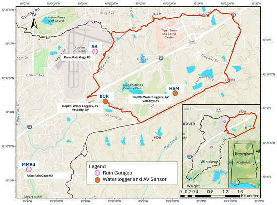
Figure 1. Study area and monitoring sites.

2.2. Data Collection and Event Selection

Rainfall and stream depth data used for model calibration were obtained from a previous study [36], including precipitation from the Airport Rain Gauge (AR) and stream observations at HAM and BCR. Rainfall was measured using an Onset HOBO R3 rain gauge (Onset Computer Corporation, Bourne, MA, USA) [37] at 5 min intervals, and stream depth was measured using Onset HOBO U20L-04 level loggers (Onset Computer Corporation, Bourne, MA, USA) [38] at 15 min intervals. The quality control of these data relied on instrument calibration and screening. Velocity data used for calibration at Hamilton Bridge (HAM) were obtained from an earlier study by [39], which measured velocity and depth using a Teledyne ISCO 2150 area-velocity sensor (Teledyne ISCO Inc., Lincoln, NE, USA) [40]. Velocity data were collected at 30 min intervals when the stream depth was below 2.54 cm (5 inches) and at 5 min intervals when it exceeded this threshold. The present study extends these records by collecting new monitoring data for independent validation and by adding field-based velocity measurements at BCR. The recorded depth and velocity measurements from the AV Sensor were used to derive head-velocity curves at HAM and BCR. In addition, discharge was also estimated at BCR using tape-measured channel cross-sectional area and velocity derived from the head-velocity (HV) rating curve. Instrument deployment details were unchanged from a prior study [18] and are not repeated here for brevity. Table 1 summarizes the datasets used to reproduce the HEC-HMS and HEC-RAS workflows.

Table 1. Monitoring stations, measured variables, and periods used for calibration and validation.

Station	Collected Field Data	Calibration Events (Rain Gauge Station: AR)	Validation Events (Rain Gauge Station: MMRd)
Hamilton Bridge (HAM)	Depth and Velocity	29 December 2021–26 January 2022	26 December 2024–23 January 2025
Bent Creek Road (BCR)	Depth and Velocity	29 December 2021–26 January 2022	4 March 2025–21 March 2025

Storm events were selected from periods with complete and time-synchronized rainfall and stream records, and the dataset was divided into calibration and validation windows. Validation periods were selected from a subset of the AV sensor deployment period to ensure that depth and velocity were measured simultaneously at the same monitoring cross-section. In contrast, the earlier calibration period relied on stream depth recorded by Onset HOBO level loggers, while velocity was estimated using a head-velocity curve developed from AV sensor measurements collected at a nearby cross-section that was slightly offset from the HOBO level logger location. The different AV sensor deployment period at two stations was due to limited AV sensor availability, and the offset in deployment location with respect to the HOBO level loggers was to place the AV sensor at a more hydraulically stable and secure site for safe operation.

In addition to the field-collected data, external datasets used in this study included a 1 m resolution digital elevation model (DEM) (Figure A3) obtained from the USDA Geospatial Data Gateway [41]. A City of Auburn (COA) high-contrast basemap was used to refine the DEM-derived stream network and to identify smaller channels and culvert crossings that were not clearly represented in the elevation data [42]. Soil information was derived from the gSSURGO database [43] to assign hydrologic soil groups. Land-use and land-cover data were obtained from the National Land Cover Database (NLCD) [44] and were used, together with soil data, to parameterize spatially distributed model inputs such as surface roughness and representative loss characteristics at the grid-cell scale.

2.3. Model Development

This study developed and compared fully distributed, two-dimensional (2D) rain-on-grid (RoG) models in HEC-HMS and HEC-RAS for extended-period watershed simulation in Moore’s Mill Creek (MMC). Both models were configured to use (i) a common terrain model, (ii) consistent precipitation time series, and (iii) aligned loss and roughness assumptions to enable direct comparison of runoff generation and overland routing behavior. Figure 2 shows the model workflow followed in this study.

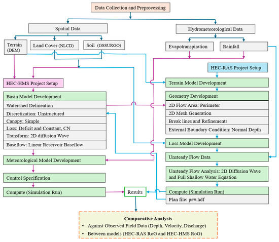
Figure 2. Schematic of basic components of model development.

2.3.1. HEC-HMS Model Development

A two-dimensional (2D) rain-on-grid (RoG) model was developed in HEC-HMS (v4.12). The DEM was imported to create the HEC-HMS terrain model, and GIS tools were used to delineate the watershed boundary using BCR as an outlet point. The initial delineation produced multiple subbasins, which were merged into a single basin element to enable a fully distributed overland-flow configuration inside the basin with flow control at BCR. Reach elements were removed so that surface routing was represented exclusively through the 2D RoG transform rather than 1D channel routing.

Continuous simulation was implemented using the Deficit and Constant Loss Method as the primary loss formulation. This choice was made to (i) support water-balance behavior as it is one of the recommended loss methods available in HEC-HMS for continuous simulation and (ii) maintain consistency with loss options available in HEC-RAS, which include SCS Curve Number, Green and Ampt, and Deficit and Constant. Here, ‘consistency’ refers to using similarly named loss formulations to support a controlled comparison, not to imply identical process representation. In HEC-HMS (single-subbasin setup in this study), losses are embedded within a continuous hydrologic soil-moisture accounting framework that produces excess precipitation for the 2D transform. In contrast, in the HEC-RAS rain-on-grid model, losses are applied cell by cell within the 2D hydraulic computation.

The Deficit and Constant method was parameterized using maximum deficit, initial deficit, percent imperviousness, and constant loss rate. Because the HEC-HMS model was configured as a single basin, one parameter set was applied for the full domain. Maximum deficit was estimated following HEC-HMS Tutorials and Guide [45] as (“Effective Porosity” − “Wilting Point”) × “Soil Depth”, with soil depth computed from NRCS Web Soil Survey (WSS) attributes [46]. Effective porosity and wilting point were selected from the HEC-HMS tutorial guidance [45] for the dominant soil texture class. The constant loss rate was estimated using area-weighted saturated hydraulic conductivity (Ksat) from WSS. Percent imperviousness was computed as an area-weighted summary of the NLCD percent imperviousness dataset in ArcGIS Pro 3.4.0. The initial deficit was treated as a calibration parameter and adjusted to improve agreement between simulated and observed runoff peak and volume.

The SCS Curve Number method, although designed for event-based simulations, is widely used in hydrologic practice because it is relatively simple and less data-intensive [47]. Therefore, in addition to the primary continuous loss formulation, the gridded SCS Curve Number (CN) method was implemented in supplementary simulations to evaluate the sensitivity of the hydrologic response to a widely used event-based loss representation and to support cross-model scenario comparisons. CN values corresponding to the average antecedent moisture condition (AMC II) were suggested by [36], with values assigned consistent with the study’s land cover and soil classification of the Moore’s Mill Creek watershed.

Subsurface contributions were represented using the linear reservoir baseflow method with two groundwater layers (GW1 representing a faster interflow component and GW2 representing a slower baseflow component). Initial discharge per unit area was set from observed pre-event flow normalized by drainage area. Groundwater storage coefficients were estimated from observed recession behavior using the linear-reservoir routing relationship [48], and manual calibration was used to adjust groundwater partition fractions and storage coefficients.

Canopy interception was represented using the Simple Canopy method. For evapotranspiration, the Monthly Average method was used for its simplicity and data availability compared to other empirical approaches. Furthermore, previous simulations without explicit calibration using the Monthly Average method produced satisfactory results in terms of hydrograph behavior for this study area. The monthly evapotranspiration rate was assigned from 20-year pan evaporation averages for the Auburn site (Southeast Ag Weather Service Center, Auburn University, Auburn, AL, USA) [49], and the crop coefficient was assumed to be 1 for simplicity. The evapotranspiration method was included in the continuous simulation for this study because it represents the mechanism by which infiltrated water is returned to the atmosphere from the canopy and the surface in the chosen Deficit and Constant Loss method.

Rainfall–runoff transformation and overland routing were simulated using the HEC-HMS 2D diffusion-wave transform on an unstructured computational mesh. It is a simplified form of the shallow-water equations in which inertial (local and convective acceleration) effects are neglected and flow is driven primarily by the water-surface slope and resisted by friction (represented through Manning-based relationships). The diffusion-wave formulation is represented as Equation (1) [11].

$${\displaystyle \frac{\partial h}{\partial t}} =\nabla ·\left(\beta \nabla z_s\right)+q$$

(1)

where $h$ is the flow depth (m), $\beta$ is the diffusivity or hydraulic conductance coefficient (m²/s), which depends on depth, roughness, and slope, $z_s$ is the water-surface elevation (m), and q is the source or sink term (m/s).

Meteorological forcing was specified using the Specified Hyetograph precipitation method based on an available gauge time series sampled at 5 min intervals. Three simulation control periods were defined to support calibration and validation: 26 December 2021 to 26 January 2022 (calibration), 23 December 2024 to 23 January 2025 (validation at HAM), and 1 March 2025 to 21 March 2025 (validation at BCR). Simulations used a 15 min computation interval, and spatial results were saved at 15 min intervals.

2.3.2. HEC-RAS Model Development

HEC-RAS (v6.3.1) was used to develop a two-dimensional (2D) rain-on-grid (RoG) model for continuous simulation. The same DEM used for the HEC-HMS 2D configuration was imported into RAS Mapper, and the watershed boundary delineated in HEC-HMS was imported to define the 2D flow-area perimeter. A base mesh with 60 m × 60 m cells was generated following prior work in the watershed [18], which showed satisfactory performance in this watershed at this scale. The mesh was locally refined along ridges, stream centerlines, and lake boundaries using breaklines and refinement regions with target cell sizes of 10–20 m, yielding approximately 15,000 cells. Elevation–area and elevation–volume relationships were precomputed for each cell from the terrain. NLCD land cover was used to spatially assign Manning’s roughness and percent imperviousness, with initial values selected based on HEC-RAS user’s manual [10]. Infiltration was represented using the Deficit and Constant method with an infiltration layer derived from NLCD land cover and gSSURGO soil data. To maintain comparability with the single-basin loss parameterization applied in HEC-HMS, a consistent set of Deficit and Constant loss parameters was applied across the modeling domain. Also, it is important to note that HEC-HMS applies loss parameterization at the subbasin level (a single parameter set in our single-subbasin configuration), whereas HEC-RAS applies losses and computations cell by cell over a 2D mesh.

Rainfall forcing used the same precipitation time series as the HEC-HMS meteorological model and was applied uniformly over the 2D mesh. A downstream external boundary condition was specified at the watershed outlet (BCR) using a normal depth, with the friction slope estimated from terrain measurements near the outlet in RAS Mapper. Internal boundary conditions were not used to maintain consistency with the HEC-HMS 2D framework used in this study. As of v4.12, HEC-HMS does not support internal boundary conditions.

To reduce dry-start sensitivity and improve reproduction of the first observed peak, a model warm-up rainfall of 30 mm was applied four days prior to the storm period in both HEC-RAS and HEC-HMS, in accordance with HEC-HMS tutorial practices [45] for initializing soil moisture. This period was not used for model evaluation. The baseline HEC-RAS simulations used the diffusion-wave solver to align with the diffusion-wave formulation used in HEC-HMS RoG. However, the 2D diffusion-wave formulation acted as a hydrologic transform in HEC-HMS, whereas it was framed as a hydraulic flow solution option inside the 2D unsteady solver in HEC-RAS. A 10 s computational time step was selected to satisfy the Courant stability criterion for the smallest refined 2D cells (10–20 m) using the maximum Courant number of 1, while maintaining computational efficiency for month-long simulations.

Calibration focused on a limited set of adjustments, including initial deficit, Manning’s roughness (iteratively varied by approximately ±10%), and refinement of breaklines and refinement regions near hydraulically sensitive locations. Terrain corrections were also applied using the Terrain Modification tool to remove unrealistic water retention and to represent pond and lake bottoms where bathymetry was not included in the original DEM. The same tool was also used to represent culverts by lowering roadway or embankment elevations along culvert alignments identified from the COA high-contrast basemap. The finalized HEC-RAS mesh and configuration (Figure A4) were then imported into the previously developed HEC-HMS model to reproduce the unstructured discretization and maintain consistent terrain, mesh, rainfall forcing, loss settings, and surface-property assumptions across platforms. HEC-HMS additionally represented baseflow and evapotranspiration. Parameters calibrated in HEC-RAS were held fixed in HEC-HMS, and further calibration in HEC-HMS was limited to baseflow parameters.

Similarly to HEC-HMS, the calibrated model was also rerun using the SCS Curve Number infiltration method, with the same CN values used in the corresponding HEC-HMS supplementary simulations, while keeping all other inputs and parameters unchanged.

Following the calibration of both models, the finalized baseline configurations (HMS-BF and RAS) were applied without further parameter adjustment to two independent validation periods at HAM and BCR.

2.4. Scenario Matrix

To compare model structures and key process assumptions, a set of scenarios was defined to test alternative loss formulations (Deficit and Constant versus SCS Curve Number) and the effect of baseflow inclusion. Table 2 summarizes the configuration of each scenario. All scenarios used the diffusion-wave formulation and baseflow was represented only in HEC-HMS.

Table 2. Scenario definitions used for model comparison.

Scenario	Loss Method	Baseflow
HMS-No BF	Deficit and Constant	Off
HMS-BF	Deficit and Constant	On
HMS-No BF-CN	SCS Curve Number	Off
HMS-BF-CN	SCS Curve Number	On
RAS	Deficit and Constant	Off
RAS-CN	SCS Curve Number	Off

2.5. Sensitivity Test

Sensitivity analyses were conducted around the calibrated baseline scenarios HMS–BF and RAS. For HEC-HMS, groundwater coefficients and fractions (GW1 and GW2), were varied within ±40% of calibrated values while preserving physical constraints, including (i) the sum of groundwater fractions not exceeding 1 and (ii) GW1 representing the faster reservoir response relative to GW2. In addition to parameter perturbations, a structural sensitivity test was performed in HEC-RAS by rerunning the calibrated model using the full shallow-water equation (SWE) while keeping all other inputs and parameters unchanged; this configuration is hereafter referred to as RAS-SWE.

2.6. Analysis

Model performance was evaluated by comparing simulated and observed hydrographs of water depth, flow velocity, and discharge for both HEC-HMS and HEC-RAS during the calibration and validation periods. Model outputs were extracted at two monitoring locations, HAM and BCR, and compared against field observations.

Model accuracy was quantified using three commonly used performance metrics: Nash–Sutcliffe efficiency (NSE), coefficient of determination (R²), and root mean square error (RMSE).

NSE was used as the primary goodness-of-fit metric because it summarizes the ability of the model to reproduce the overall hydrograph shape and variability relative to the observed mean. NSE was computed as follows:

$$\mathrm{NSE}=1-{\displaystyle \frac{{\sum }_{i=1}^n({OBS}_i-SI{M}_i{)}^2}{{\sum }_{i=1}^n({OBS}_i-\overline{OBS}{)}^2}}$$

(2)

where $OB{S}_i$ and $SI{M}_i$ are the observed and simulated values at time $i$, $\overline{OBS}$ is the mean of the observed series, and $n$ is the number of observations. NSE values range from $-\mathrm{\infty }$ to 1, with values closer to 1 indicating better agreement. Model performance was interpreted using the criteria of [50]: very good (0.75–1.00), good (0.65–0.75), satisfactory (0.50–0.65), and unsatisfactory (≤0.50).

R² was used to quantify the degree of linear association between simulated and observed values and to indicate how well the model reproduced the variance in observations. R² was computed as follows:

$${\mathrm{R}}^2={\left[{\displaystyle \frac{{\sum }_{i=1}^n({OBS}_i-\overline{OBS})(SI{M}_i-\overline{SIM})}{\sqrt{{\sum }_{i=1}^n({OBS}_i-\overline{OBS}{)}^2}\sqrt{{\sum }_{i=1}^n(SI{M}_i-\overline{SIM}{)}^2}}}\right]}^2$$

(3)

where $\overline{SIM}$ is the mean of simulated values. R² was interpreted alongside NSE and volumetric diagnostics because it does not, by itself, distinguish systematic bias (under- or overestimation) and can be influenced by outliers.

RMSE was used to quantify the average magnitude of error in the original units of the simulated variable, with larger errors weighted more heavily due to squaring. RMSE was computed as follows:

$$\mathrm{RMSE}=\sqrt{{\displaystyle \frac{1}{n}}\sum _{i=1}^n({OBS}_i-SI{M}_i{)}^2}$$

(4)

Lower RMSE values indicate closer agreement between simulated and observed time series, while higher values indicate larger typical deviations, particularly during periods such as peaks and recession limbs where errors can be amplified.

Percent Bias (PBIAS, %) was employed to assess the systematic bias of depth, velocity, and discharge simulations. A positive PBIAS value indicates overestimation, whereas a negative PBIAS value indicates underestimation, and a PBIAS value of 0 indicates a perfect case. PBIAS was computed as follows:

$$\mathrm{P}\mathrm{B}\mathrm{I}\mathrm{A}\mathrm{S}=100\times {\displaystyle \frac{{\sum }_{i=1}^n({SIM}_i-{OBS}_i)}{{\sum }_{i=1}^n\left({OBS}_i\right)}}$$

(5)

In addition to hydrograph-based evaluation, event runoff volumes were computed by integrating discharge over each storm event. An effective runoff coefficient was calculated as the ratio of runoff volume to rainfall volume over the catchment. Storm events were separated using an inter-event dry period of 6 h, and event runoff coefficients were summarized as a time series using the event end time.

Sensitivity test results for HEC-HMS were analyzed relative to the baseline configuration by comparing changes in the NSE and cumulative runoff volume.

3. Results

3.1. Calibration Results

3.1.1. Loss Method: Deficit and Constant

Figure 3 compares simulated depth hydrographs at HAM (Figure 3a) and BCR (Figure 3b) using the Deficit and Constant Loss method. It is noticed that HMS-BF tends to capture peak depths better relative to the observations (OBS) than the other models. Adding baseflow in HEC-HMS (HMS-BF) increases peak depth relative to the no-baseflow case (HMS-No BF) by 24% on average at HAM and by 54% on average at BCR. HMS-BF captured the overall hydrograph behavior, including peak depth and recession patterns, better than HMS-No BF. Because HMS-No BF and HEC-RAS share the same mesh, terrain, loss method, and 2D diffusion-wave transform, their simulated hydrographs are broadly similar. The small differences that are visible likely arise from software-specific numerical implementations and internal handling of cell-averaged quantities. Table 3 also compares the depth errors at the two stations and shows that HMS-BF provides better agreement with the observed depth hydrographs at both stations, indicating the importance of including baseflow in the model.

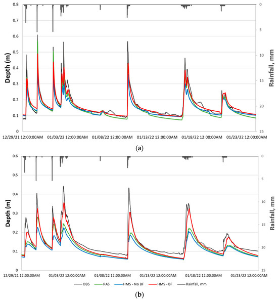
Figure 3. Comparison of depth hydrographs at (a) HAM and (b) BCR using Deficit and Constant Loss method.

Table 3. Comparison of depth errors for HAM and BCR monitoring sites using Deficit and Constant Loss method.

Scenario	NSE		R2		RMSE (m)		PBIAS (%)
	HAM	BCR	HAM	BCR	HAM	BCR	HAM	BCR
RAS	0.82	0.59	0.88	0.78	0.03	0.04	−11.7	−19.3
HMS-No BF	0.74	0.41	0.9	0.81	0.04	0.05	−11.8	−26.37
HMS-BF	0.89	0.83	0.9	0.88	0.02	0.03	−1.22	−10.75

Similarly to the depth results, adding baseflow (HMS-BF) produced higher inter-event velocities and a more prolonged recession at both HAM (Figure 4a) and BCR (Figure 4b) relative to the no-baseflow case (HMS-No BF) and RAS. This also improved the evaluation statistics (higher NSE and R² and lower RMSE and PBIAS) (Table 4), while peak timing remained comparable between scenarios. The main station-level difference was velocity persistence between storms. At HAM, HMS-BF showed a slightly raised baseline compared to HMS-No BF and RAS, but simulated velocities still remained below the observed baseline during extended dry periods (Figure 4a), whereas this behavior was not apparent at BCR under the same rainfall forcing (Figure 4b). This discrepancy likely reflects observational and geometric differences at HAM because observed velocities were obtained by applying a rating curve developed from AV depth–velocity measurements in 2024 to HOBO depths recorded slightly upstream during the 2021–2022 calibration period. Because the HOBO deployment cross-section was deeper than the AV sensor cross-section, the transferred rating curve may introduce systematic bias in the derived velocities. While this was the same for BCR, cross-sections at two deployments were very similar at BCR.

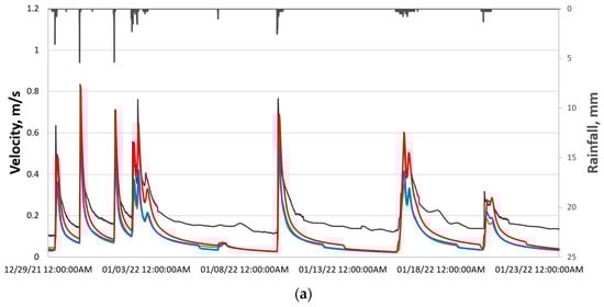
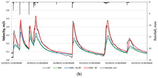
Figure 4. Comparison of velocity hydrographs at (a) HAM and (b) BCR using Deficit and Constant Loss method.

Table 4. Comparison of velocity errors for HAM and BCR monitoring sites using Deficit and Constant Loss method.

Scenario	NSE		R2		RMSE (m/s)		PBIAS (%)
	HAM	BCR	HAM	BCR	HAM	BCR	HAM	BCR
RAS	−0.43	0.64	0.87	0.85	0.11	0.06	−55.7	−20.18
HMS-No BF	−0.36	0.73	0.89	0.89	0.11	0.05	−54.6	−15.9
HMS-BF	0.15	0.9	0.89	0.91	0.09	0.03	−39.0	6.46

Figure 5 shows the discharge hydrographs generated by HEC-RAS and HEC-HMS using the Deficit and Constant Loss method. The HEC-HMS simulation with linear reservoir baseflow (HMS-BF) shows the closest agreement with observed discharge, capturing storm peaks and sustaining inter-event flows. In contrast, the HMS-No BF and RAS simulations both underestimate the observed discharge between events. This might be because neither of them incorporates groundwater return flow, so any infiltrated rain is treated as a permanent loss from the surface system. Table 5 compares the discharge errors for various scenarios at BCR monitoring sites. NSE and RMSE improved significantly with the addition of baseflow components.

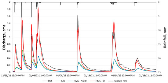
Figure 5. Comparison of discharge hydrograph at BCR using Deficit and Constant Loss method.

Table 5. Comparison of discharge errors for BCR monitoring site using Deficit and Constant Loss method.

Scenario	NSE	R2	RMSE (m3/s)	PBIAS (%)
RAS	0.25	0.72	0.25	−58.9
HMS-No BF	0.18	0.8	0.26	−64.7
HMS-BF	0.91	0.94	0.09	−13.6

3.1.2. Loss Method: SCS Curve Number Method

Figure 6 shows depth, velocity, and discharge hydrographs from the CN simulations. For the first two peaks, the HEC-HMS scenario with baseflow shows better agreement with observations than the scenario without baseflow and the HEC-RAS scenario for depth, velocity, and discharge. After the first major storm sequence, the two HEC-HMS scenarios behave almost identically and both overshoot the observed peaks, whereas no such spikes are visible in the HEC-RAS scenario. Over the extended simulation, the RAS-CN scenario shows more satisfactory performance than the comparable HEC-HMS scenario for depth and velocity (NSE = 0.59 and 0.64) (Figure 6a,b). However, discharge remains underpredicted (NSE = 0.25) (Figure 6c), likely due to the lack of a loss recovery option. Although both models used the same CN grids and the same routing method, these differences likely result from model-specific implementations of the CN loss method, particularly the treatment of soil moisture settings for the same CN grids.

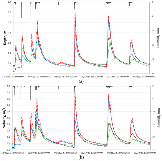
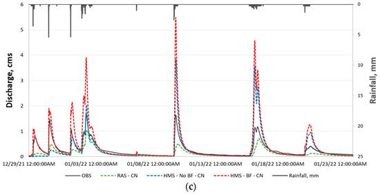
Figure 6. Comparison of (a) depth, (b) velocity, and (c) discharge hydrographs at BCR using the SCS Curve Number Loss method.

3.2. Validation Results

Table 6 indicates a very good statistical performance during the validation period at HAM. Figure 7 shows that the model reproduces the observed hydrograph behavior, including time to peak, recession, and overall shape. The lower baseline velocities noted during calibration (Figure 4a) are not apparent in validation (Figure 7b), likely because the validation analysis uses depth and velocity extracted directly from the AV sensor location, unlike during the calibration period, where they were not collocated.

Table 6. Comparison of depth and velocity errors for HAM monitoring site using Deficit and Constant Loss method for validation period.

	Scenario	NSE	R2	RMSE	PBIAS (%)
Depth	RAS	0.81	0.87	0.03	−2.04
	HMS-BF	0.9	0.92	0.02	8.03
Velocity	RAS	0.64	0.86	0.05	−24.26
	HMS-BF	0.83	0.9	0.04	−12.5

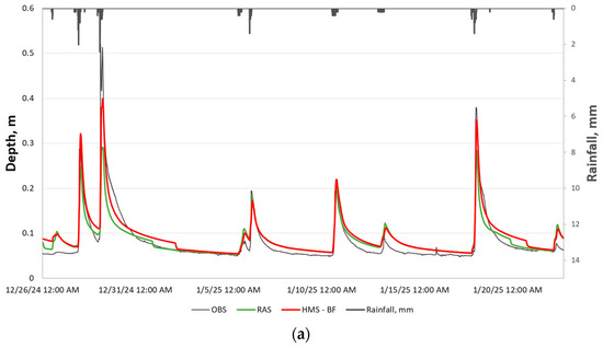
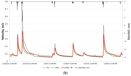
Figure 7. Comparison of (a) depth and (b) velocity hydrographs at HAM using Deficit and Constant Loss method for validation period.

Table 7 compares discharge hydrograph performance at BCR across the two models and shows degraded performance relative to the calibration period (Table 5). In validation, the simulated hydrograph deviates from observations on the rising limb and in the time to peak (Figure 8). This timing mismatch is likely driven by spatial rainfall variability because the rain data used for validation was from the MMRd Station, and it is possible that the rain started slightly later at this station than at the BCR location, causing a shift in timing. Furthermore, the processing used to smooth irregularities in the AV sensor record may have shifted the observed hydrograph earlier. The inflated first peak may also reflect that antecedent precipitation added during calibration appears to be ineffective for the validation storm and may require recalibration.

Table 7. Comparison of discharge errors for BCR monitoring site using Deficit and Constant Loss method for validation period.

Scenario	NSE	R2	RMSE	PBIAS (%)
RAS	0.21	0.47	0.97	−72.4
HMS-BF	0.21	0.28	0.97	−64.6

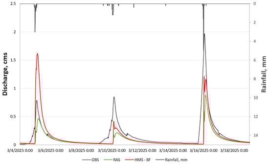
Figure 8. Comparison of discharge hydrograph at BCR using Deficit and Constant Loss method for validation period.

3.3. Sensitivity Results

Figure 9 shows the sensitivity of HEC-HMS to groundwater parameters. NSE is more sensitive to the groundwater fractions than to the coefficients (Figure 9a). Increasing the GW fractions from the calibrated value increased return flow and cumulative volume (Figure 9b) while degrading NSE, suggesting that routing a larger share of infiltrated water to the groundwater reservoirs increases total volume. In contrast, GW1 and GW2 coefficients have a negligible influence on cumulative volume and only a modest influence on NSE (maximum change of about 6% for a −40% change in the GW2 coefficient) (Figure 9a). This might be because GW coefficients primarily control the rate at which stored water is released. Accordingly, increasing the coefficients mainly redistributes the flow in time by attenuating peaks and extending recessions, while leaving the overall volume nearly unchanged.

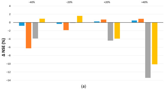
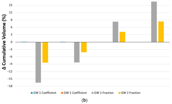
Figure 9. Sensitivity analysis of HEC-HMS baseflow parameters: (a) discharge-based change in NSE with respect to baseline model, (b) cumulative volume difference relative to baseline simulation at BCR monitoring site.

Figure 10 shows that under identical terrain, mesh, loss method, and land cover scenarios, the two solvers produce different hydrographs. The trends in the rising and falling of the hydrographs are similar in both solvers. However, the model using full shallow-water equations fails to achieve the base water level. This might be because diffusion-wave solutions tend to move water more slowly and spread it out in time. As a result, to move the same volume at slower velocities, the system often compensated by holding more water, leading to higher depths compared to SWE. However, an earlier study by [18] in the same watershed, calibrated using a full shallow-water equation, showed satisfactory results, but required much effort to adjust the cross-sections of DEM and inclusion of low flow discharge through internal boundary conditions to match the baseline depths or velocities.

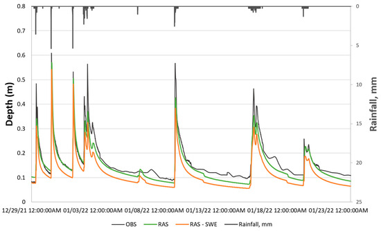
Figure 10. Sensitivity analysis of HEC-RAS model to solver settings at HAM, diffusion-wave equation and full shallow-water equation (SWE).

3.4. Cumulative Volume Comparison

The cumulative runoff volume curves in Figure 11a show differences between the HEC-RAS and HEC-HMS scenarios. Enabling baseflow in HEC-HMS introduces a continuous groundwater contribution, which substantially increases the cumulative volume curves. Because HEC-RAS does not include a baseflow component, its cumulative runoff volume is lower than the HEC-HMS with-baseflow scenario for the same loss method. The loss method also strongly influences runoff volume. The SCS Curve Number method produces higher cumulative runoff than the Deficit and Constant method in both models. However, the difference is greater in HEC-HMS than in HEC-RAS. This is likely because these two software handle soil moisture settings differently for the same CN grids as mentioned earlier.

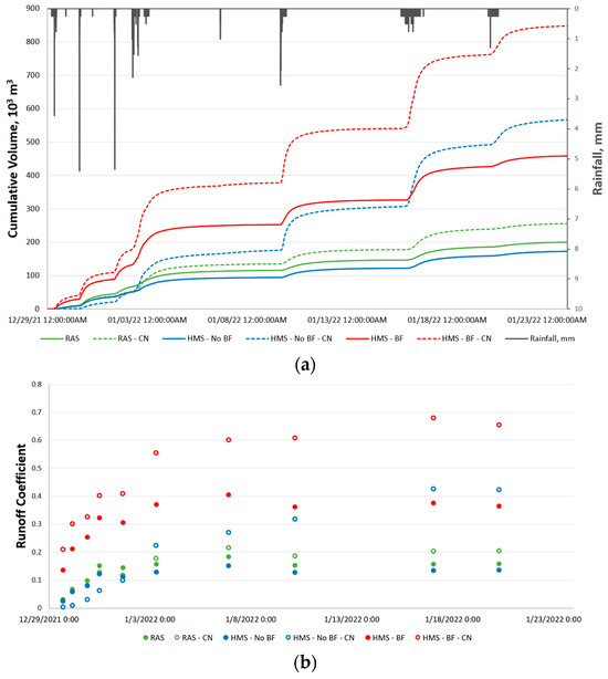
Figure 11. Comparison of (a) cumulative runoff volume and (b) runoff coefficients at BCR monitoring site for different scenarios.

The time-varying runoff coefficient (Figure 11b) shows the dynamic runoff response, which differs between models and loss methods. All scenarios exhibit low initial runoff coefficients at the onset of rainfall, and the runoff coefficient rises non-linearly during each rainfall event. The CN-based simulations reach a higher peak runoff coefficient than their Deficit and Constant counterparts, particularly in prolonged storms for HEC-HMS. This is likely because once the CN loss method’s initial retention is satisfied, additional rainfall is converted mainly to runoff. In contrast, the Deficit and Constant method continues to infiltrate at a constant rate even after saturation, which moderates the rise in the runoff fraction. Baseflow effects are also clearly reflected in the trends of the runoff coefficient.

4. Discussion and Conclusions

In this study, the rain-on-grid comparison between HEC-HMS 2D and HEC-RAS 2D used an identical unstructured mesh, loss parameters, and 2D routing formulation. Under this shared geometric foundation, differences in simulated hydrographs are most plausibly attributed to differences in hydrologic accounting, particularly baseflow and loss-method state handling, rather than to differences in terrain processing or channel routing structure. Although both models produced satisfactory to very good depth and velocity results based on NSE classifications, their outputs displayed clear differences when the model configurations were varied.

One of the most important distinctions between HEC-HMS 2D and HEC-RAS 2D affecting the multi-event simulations in the present study was baseflow representation. In HEC-HMS, the Deficit and Constant Loss method conceptualizes soil storage and percolation, and the HEC-HMS User’s Manual [27] indicates that percolation is lost from the system unless the linear reservoir baseflow method is used, in which case percolation becomes baseflow at the outlet. Consistent with this process representation, enabling linear-reservoir baseflow improved recession behavior and increased inter-event flow persistence and cumulative runoff volume relative to surface-only configurations in HEC-RAS, which underpredicted them. This contrast gives insight into a broader limitation when hydraulic models such as HEC-RAS are applied to extended-period watershed simulation. Although these models are highly effective at representing flood wave propagation, spatially distributed inundation, and peak timing, as shown by studies [9,12,15], they lead to biased water balances and unrealistic, low flow in rain-on-grid configurations. This finding is consistent with recent studies that emphasize the importance of representing groundwater in continuous modeling. For example, Ref. [18] compared scenarios with and without a groundwater module in a semi-urban watershed using SWMM and showed that including a baseflow component substantially improved the overall water balance. Similarly, Ref. [51] reported that combining a soil-moisture accounting loss method with a linear reservoir baseflow option in HEC-HMS yielded more realistic runoff volumes and recession behavior. Together, these results indicate that explicit baseflow representation is a key requirement for extending rain-on-grid frameworks beyond event-based flood analysis toward continuous watershed simulation.

Differences between the SCS Curve Number and Deficit and Constant configurations indicate that multi-event rain-on-grid performance is strongly controlled by how soil-water state and recovery are represented. The HEC-HMS Technical Reference Manual [29] notes that the CN method includes no mechanism to extract infiltrated water and therefore “should only be used for event simulation.” This provides a plausible explanation for the progressive increase in runoff response observed in the HMS-CN simulations over multi-storm periods. As cumulative rainfall increases, infiltration approaches the maximum retention (S), and subsequent rainfall is converted more efficiently to direct runoff. Because soil drying and evapotranspiration-driven recovery are not represented within this event-oriented formulation, storage does not fully recover between storms, leading to reasonable early hydrographs but exaggerated peaks later and a biased water balance. In contrast, Deficit and Constant is described as enabling continuous simulation when paired with a canopy method that removes soil water in response to potential evapotranspiration, allowing soil storage to dry between events and stabilizing storm-to-storm response [29]. Differences between HMS-CN and RAS-CN over later storms are also consistent with the fact that HEC-RAS modifies the CN method by including a recovery approach that resets cumulative rainfall depth to zero after a user-specified dry-time period [27]. In this study, applying event separation in HEC-RAS reduced late-period runoff amplification and improved hydrograph shape, although cumulative volume remained biased (Figure 6c). Therefore, even with identical CN grids, CN behavior is not expected to be equivalent across platforms in multi-event simulations, and the results reinforce that extended-period realism depends more on loss-method state, recovery mechanisms, and baseflow representation than on routing alone.

Baseflow sensitivity results are interpretable through the parameter roles defined in the HEC-HMS linear-reservoir method. The technical reference manual [29] notes that the method uses infiltrated volume as inflow and partitions it across one to three reservoirs using partition fractions; routing coefficients then control how quickly each reservoir drains and therefore shape recession timing. This provides a direct explanation for the outcome that cumulative volume was more sensitive to groundwater fractions than to coefficients. The solver sensitivity results are also best framed as a structural modeling choice rather than a minor numerical preference. The observed divergence in baseline depths between diffusion-wave and SWE configurations shows that the choice of equation set can influence the inferred low-flow behavior under rain-on-grid models, even with identical terrain and infiltration layers. The model results were also heavily influenced by cross-sections.

The results also indicate that the event-scale runoff coefficients computed from the continuous HEC-HMS 2D simulations varied from storm to storm in response to antecedent soil moisture and storm intensity. Before larger storm events, the soil-moisture accounting module indicated higher saturation, which led to higher runoff efficiency. This behavior is consistent with previous PCSWMM applications in the same watershed, which calculated time-varying runoff coefficients and reported a systematic increase in runoff fraction as the catchment became progressively wetter [18], similar to the pattern observed in our simulations. Compared with HEC-HMS 2D results, the PCSWMM models tend to produce somewhat higher runoff coefficients. However, these differences are likely influenced by differences in model configuration, loss methods, calibration strategy, and most importantly, monitoring locations, so a strict one-to-one comparison is not possible. A study in the Ohio River region by [52] also examined tens of thousands of rainfall–runoff events and found that the same watershed can generate a small runoff fraction during one storm and a much larger fraction during a subsequent storm when the soil is wet, further reinforcing that runoff coefficients are highly event-dependent. In contrast, design approaches that rely on a single runoff coefficient for each land-use category, such as the traditional Rational Method, cannot represent this dependence on antecedent conditions and storm sequencing, a limitation that is also acknowledged in Ref. [53]. In addition, different scenarios in this study showed that the use of the CN loss method (HMS-No BF-CN, HMS-BF-CN, RAS-CN) consistently yielded higher cumulative volumes and higher event runoff coefficients than the corresponding Deficit and Constant runs, which indicates a lower effective infiltration capacity in CN-based formulations. However, since CN in this study was not calibrated, but instead imported directly from a QGIS CN look-up value presented by [18,36], it might be inappropriate to draw conclusions about this. Furthermore, turning on the baseflow module (HMS-BF and HMS-BF-CN) further increased both cumulative discharge and event runoff coefficients compared with the no baseflow cases, because groundwater discharge also added to stormflow volume. Taken together, these patterns also show that the effective runoff coefficient in this semi-urban catchment is a dynamic outcome of antecedent soil moisture, baseflow state, rainfall intensity, and the chosen loss formulation, rather than an intrinsic constant tied only to land use.

The findings thus guide us toward the goal of analyzing surface hydrology parameters, such as depth and velocity, for multi-event simulations where inter-event recession and cumulative volumes are important. The improved realism yielded by HEC-HMS 2D is important for the modeling of water balance in watersheds in extended-period simulations. Moreover, it is hoped that this model will support future studies tracking the generation and motion of sediment within the watershed.

5. Limitations and Recommendations for Future Works

5.1. Limitations

Despite using identical rain-on-grid forcing, the same unstructured mesh, and closely aligned numerical settings, the comparison between HEC-HMS 2D and HEC-RAS 2D is constrained by limited observational control and shared sources of uncertainty. Discharge was observed only at the outlet near Bent Creek Road (BCR), so calibration and evaluation were anchored to a single outlet hydrograph, while the evaluation at Hamilton (HAM) relied on depth and velocity time series and therefore did not provide an independent discharge or water-balance constraint.

Discharge estimates were further affected by rating-curve uncertainty, which is often largest at high flows and during recessions [54], and by potential noise or bias in area-velocity measurements associated with flow conditions, acoustic scatterers, sensor alignment, and fouling [55]. Rainfall forcing was another limitation because spatial and temporal variability in precipitation strongly controls runoff generation [56], and any bias in storm structure, timing, or magnitude in the rainfall product propagated to both models, as seen in Figure 8.

In addition, deficit and constant loss parameters were uniform across the watershed; therefore, spatial variability in infiltration capacity was not fully represented. Another limitation of this study relates to field data availability. Occasional instrument failures, particularly rainfall measurements, resulted in data gaps that prevented the use of longer continuous simulation periods for calibration. Consequently, calibration was limited to windows for which complete and reliable rainfall and in-stream observations were available. Furthermore, environmental sensitivity of instrumentation and uncertainty in terrain representation, including microtopography, channel geometry, and sensor elevation referencing, can affect simulated stages and velocities, as seen in Figure 4a.

5.2. Recommendations for Future Work

Future work should test the generalizability of these findings by extending the intercomparison to longer simulation windows across multiple seasons and hydrometeorological conditions, thereby evaluating the stability and transferability of calibrated parameters such as baseflow and roughness. Additional experiments should separate forcing uncertainty from structural model differences by repeating the analysis with alternative rainfall products, such as those from [57,58], and by systematically varying temporal resolution to quantify sensitivity to time-step selection.

As mentioned earlier, the comparison should also be strengthened by increasing internal model structure, for example, by subdividing the watershed into multiple subbasins and junctions so that distributed flow behavior can also be evaluated at interior locations rather than primarily at a single outlet. In parallel, performance and practicality should be assessed across modeling complexity options by comparing fully 2D rain-on-grid configurations with semi-distributed HEC-HMS formulations using lumped subbasin parameters and empirical unit hydrographs, with explicit accounting for accuracy gains versus computational cost. Process representation can be further tested by evaluating alternative loss and soil-water accounting schemes within HEC-HMS (for example, Green–Ampt infiltration or soil-moisture accounting).

Furthermore, this work can be extended by comparing HEC-HMS 2D with widely used urban watershed models, such as SWMM, under consistent forcing and observation datasets to assess model suitability. Finally, linking hydrologic simulations to sediment transport or water-quality modules would expand the management relevance by testing whether improved spatiotemporal flow fields translate into realistic predictions of erosion, sediment yield, and deposition patterns.

References

- Redfern, T.W.; Macdonald, N.; Kjeldsen, T.R.; Miller, J.D.; Reynard, N. Current Understanding of Hydrological Processes on Common Urban Surfaces. Prog. Phys. Geogr. 2016, 40, 699–713. [Google Scholar] [CrossRef]
- Jacobson, C.R. Identification and Quantification of the Hydrological Impacts of Imperviousness in Urban Catchments: A Review. J. Environ. Manag. 2011, 92, 1438–1448. [Google Scholar] [CrossRef]
- Cristiano, E.; ten Veldhuis, M.C.; van de Giesen, N. Spatial and Temporal Variability of Rainfall and Their Effects on Hydrological Response in Urban Areas: A Review. Hydrol. Earth Syst. Sci. 2017, 21, 3859–3878. [Google Scholar] [CrossRef]
- Moors, E.J.; Grimmond, C.S.B.; Veldhuizen, A.B.; Järvi, L.; van der Bolt, F. Urban Water Balance and Hydrology Models to Support Sustainable Urban Planning. In Understanding Urban Metabolism: A Tool for Urban Planning; Chrysoulakis, N., de Castro, E.A., Moors, E.J., Eds.; Routledge: London, UK, 2014; pp. 106–116. [Google Scholar]
- Jones, J.A.A. Global Hydrology: Processes, Resources and Environmental Management; Routledge: London, UK, 2014; 414p. [Google Scholar] [CrossRef]
- Vasconcelos, J.G.; Fang, X.; Geller, V.G.; Nicolaico, G.G.; Reyes, E.M. NCHRP Synthesis 602: Resilient Design with Distributed Rainfall-Runoff Modeling; Transportation Research Board, National Academies of Sciences, Engineering, and Medicine; The National Academies Press: Washington, DC, USA, 2023. [Google Scholar] [CrossRef]
- Wolff-Piggott, B. Demonstrating the Potential of GIS Technology in Hydrosalinity Modelling Through Interfacing the DISA Model and a GIS; WRC Report No. 588/1/95; Water Research Commission (WRC): Pretoria, South Africa, 1995. Available online: https://www.wrc.org.za/wp-content/uploads/mdocs/588-1-95.pdf (accessed on 30 December 2025).
- Beven, K. Changing Ideas in Hydrology: The Case of Physically-Based Models. J. Hydrol. 1989, 105, 157–172. [Google Scholar] [CrossRef]
- Costabile, P.; Macchione, F.; Natale, L.; Petaccia, G. Flood Mapping Using LiDAR DEM: Limitations of the 1-D Modeling Highlighted by the 2-D Approach. Nat. Hazards 2015, 77, 181–204. [Google Scholar] [CrossRef]
- Hydrologic Engineering Center. HEC-RAS User’s Manual; U.S. Army Corps of Engineers: Washington, DC, USA, 2025. Available online: https://www.hec.usace.army.mil/confluence/rasdocs/rasum/latest (accessed on 9 November 2025).
- U.S. Army Corps of Engineers; Hydrologic Engineering Center (HEC). HEC-RAS Hydraulic Reference Manual; Version 6.0 Beta; CPD-69; USACE Hydrologic Engineering Center: Davis, CA, USA, 2020. Available online: https://www.hec.usace.army.mil/confluence/rasdocs/ras1dtechref/latest (accessed on 24 November 2025).
- Costabile, P.; Costanzo, C.; Ferraro, D.; Barca, P. Is HEC-RAS 2D Accurate Enough for Storm-Event Hazard Assessment? Lessons Learnt from a Benchmarking Study Based on Rain-on-Grid Modelling. J. Hydrol. 2021, 603, 126962. [Google Scholar] [CrossRef]
- Ennouini, W.; Fenocchi, A.; Petaccia, G.; Persi, E.; Sibilla, S. A Complete Methodology to Assess Hydraulic Risk in Small Ungauged Catchments Based on HEC-RAS 2D Rain-On-Grid Simulations. Nat. Hazards 2024, 120, 7381–7409. [Google Scholar] [CrossRef]
- Afshari, S.; Tavakoly, A.A.; Rajib, M.A.; Zheng, X.; Follum, M.L.; Omranian, E.; Fekete, B.M. Comparison of New Generation Low-Complexity Flood Inundation Mapping Tools with a Hydrodynamic Model. J. Hydrol. 2018, 556, 539–556. [Google Scholar] [CrossRef]
- Bratton, A.J. A Comparison of 1D and 2D HEC-RAS Models of the Napa River Through the City of St. Helena, California. Master’s Thesis, California State University, Sacramento, CA, USA, 2017. [Google Scholar]
- Odey, G.; Cho, Y. Event-Based vs. Continuous Hydrological Modeling with HEC-HMS: A Review of Use Cases, Methodologies, and Performance Metrics. Hydrology 2025, 12, 39. [Google Scholar] [CrossRef]
- Miller, M.P.; Buto, S.G.; Susong, D.D.; Rumsey, C.A. The Importance of Base Flow in Sustaining Surface Water Flow in the Upper Colorado River Basin. Water Resour. Res. 2016, 52, 3547–3562. [Google Scholar] [CrossRef]
- Bragg, M.A.; Poudel, A.; Vasconcelos, J.G. Comparing SWMM and HEC-RAS Hydrological Modeling Performance in Semi-Urbanized Watershed. Water 2025, 17, 1331. [Google Scholar] [CrossRef]
- Godara, N.; Bruland, O.; Alfredsen, K. Comparison of Two Hydrodynamic Models for Their Rain-on-Grid Technique to Simulate Flash Floods in Steep Catchment. Front. Water 2024, 6, 1384205. [Google Scholar] [CrossRef]
- Castaneda Galvis, L.F. Effect of Hydrologic and Hydraulic Calculation Approaches on Pier Scour Estimates. Master’s Thesis, Auburn University, Auburn, AL, USA, 9 December 2023. [Google Scholar]
- Zeiger, S.J.; Hubbart, J.A. Measuring and Modeling Event-Based Environmental Flows: An Assessment of HEC-RAS 2D Rain-on-Grid Simulations. J. Environ. Manag. 2021, 285, 112125. [Google Scholar] [CrossRef]
- Zhang, Z. Performance of Long-Term Continuous Hydrological Models in Fluvial Flow Simulation in a Large-Scale River Basin. Sci. Rep. 2025, 15, 22124. [Google Scholar] [CrossRef]
- Sánchez-Gómez, A.; Schürz, C.; Molina-Navarro, E.; Bieger, K. Groundwater Modelling in SWAT+: Considerations for a Realistic Baseflow Simulation. Groundw. Sustain. Dev. 2024, 26, 101275. [Google Scholar] [CrossRef]
- Hossain, S.; Hewa, G.A.; Wella-Hewage, S. A Comparison of Continuous and Event-Based Rainfall–Runoff (RR) Modelling Using EPA-SWMM. Water 2019, 11, 611. [Google Scholar] [CrossRef]
- Jaber, F.H.; Shukla, S. MIKE SHE: Model Use, Calibration, and Validation. Trans. ASABE 2012, 55, 1479–1489. [Google Scholar] [CrossRef]
- Fattahi, A.M.; Hosseini, K.; Farzin, S.; Mousavi, S.F. An Innovative Approach of GSSHA Model in Flood Analysis of Large Watersheds Based on Accuracy of DEM, Size of Grids, and Stream Density. Appl. Water Sci. 2022, 13, 33. [Google Scholar] [CrossRef]
- Hydrologic Engineering Center (HEC). HEC-HMS User’s Manual; U.S. Army Corps of Engineers: Washington, DC, USA, 2025. Available online: https://www.hec.usace.army.mil/confluence/hmsdocs/hmsum/latest (accessed on 10 November 2025).
- Sahu, M.K.; Shwetha, H.R.; Dwarakish, G.S. State-of-the-Art Hydrological Models and Application of the HEC-HMS Model: A Review. Model. Earth Syst. Environ. 2023, 9, 3029–3051. [Google Scholar] [CrossRef]
- Hydrologic Engineering Center (HEC). HEC-HMS Technical Reference Manual; U.S. Army Corps of Engineers: Washington, DC, USA, 2025. Available online: https://www.hec.usace.army.mil/confluence/hmsdocs/hmstrm/ (accessed on 9 November 2025).
- Evaluation of the Two-Dimensional Hydrological Model HEC-HMS in a Mediterranean Semiarid Basin. Available online: https://www.iahr.org/library/infor?pid=31065 (accessed on 17 December 2025).
- U.S. Environmental Protection Agency (EPA). Clean Water Act Section 303(d): Impaired Waters and Total Maximum Daily Loads (TMDLs). Available online: https://www.epa.gov/tmdl (accessed on 23 January 2026).
- Alabama Department of Environmental Management (ADEM). 2024 Alabama §303(d) List; Alabama Department of Environmental Management: Montgomery, AL, USA, 2024. Available online: https://adem.alabama.gov/programs/water/wquality/2024AL303dList.pdf (accessed on 30 December 2025).
- Climate-Data.org. Auburn Climate: Weather Auburn & Temperature by Month. Available online: https://en.climate-data.org/north-america/united-states-of-america/alabama/auburn-17365/ (accessed on 7 December 2025).
- National Centers for Environmental Information (NCEI). U.S. Monthly Climate Normals (1991–2020): Monthly Maximum, Minimum, and Average Temperature; Precipitation; Snowfall for Station USC00016129; National Oceanic and Atmospheric Administration (NOAA): Asheville, NC, USA, 2021. Available online: https://www.ncei.noaa.gov/access/services/data/v1?dataTypes=MLY-TMAX-NORMAL%2CMLY-TMIN-NORMAL%2CMLY-TAVG-NORMAL%2CMLY-PRCP-NORMAL%2CMLY-SNOW-NORMAL&dataset=normals-monthly-1991-2020&format=pdf&stations=USC00016129 (accessed on 23 January 2026).
- Acer Engineering, LLC. Moore’s Mill Creek Watershed Management Plan, Lee County, Alabama; Acer Environmental, Inc.: Atlanta, GA, USA, 2008. [Google Scholar]
- Xiao, H. Evaluating Alternatives for the Implementation of Curve Number in SWMM for an Urbanized Watershed. Master’s Thesis, Auburn University, Auburn, AL, USA, 10 December 2022. [Google Scholar]
- Onset (HOBO). Rain Gauge Data Logger RG3. Available online: https://www.onsetcomp.com/products/data-loggers/rg3 (accessed on 18 December 2025).
- Onset (HOBO). Water Level Data Logger U20L-0x. Available online: https://www.onsetcomp.com/products/data-loggers/u20l-0x (accessed on 18 December 2025).
- Bragg, M.A. Modeling Hydrology and Water Quality in Moore’s Mill Creek Using the Storm Water Management Model (SWMM). Master’s Thesis, Auburn University, Auburn, AL, USA, 10 May 2025. [Google Scholar]
- Teledyne ISCO. 2150 Area Velocity Module. Available online: https://www.teledyneisco.com/water-and-wastewater/2150-area-velocity-module (accessed on 18 December 2025).
- U.S. Department of Agriculture, Natural Resources Conservation Service (USDA NRCS). Geospatial Data Gateway. Available online: https://datagateway.nrcs.usda.gov/ (accessed on 30 December 2025).
- City of Auburn, Alabama. City of Auburn Map. Available online: https://webgis.auburnalabama.org/coamap/ (accessed on 24 November 2025).
- United States Department of Agriculture. Soil Survey Geographic Database (SSURGO). Available online: https://data.nal.usda.gov/dataset/soil-survey-geographic-database-ssurgo (accessed on 30 December 2025). [CrossRef]
- U.S. Geological Survey, Earth Resources Observation and Science (EROS) Center. Annual National Land Cover Database. 2024. Available online: https://www.usgs.gov/centers/eros/science/annual-national-land-cover-database (accessed on 30 December 2025).
- Hydrologic Engineering Center (HEC). HEC-HMS Tutorials and Guides; U.S. Army Corps of Engineers: Washington, DC, USA, 2025. Available online: https://www.hec.usace.army.mil/confluence/hmsdocs/hmsguides (accessed on 18 December 2025).
- USDA Natural Resources Conservation Service (NRCS). Web Soil Survey. Available online: https://websoilsurvey.nrcs.usda.gov/app/ (accessed on 9 November 2025).
- Fanta, S.S.; Tadesse, S.T. Application of HEC–HMS for Runoff Simulation of Gojeb Watershed, Southwest Ethiopia. Model. Earth Syst. Environ. 2022, 8, 4687–4705. [Google Scholar] [CrossRef]
- Clark, C.O. Storage and the Unit Hydrograph. Trans. Am. Soc. Civ. Eng. 1945, 110, 1419–1446. [Google Scholar] [CrossRef]
- Alabama Cooperative Extension System (ACES), Auburn University. Pan Evaporation in Alabama: 20-Year Averages for Selected Sites. Available online: https://ssl.acesag.auburn.edu/anr/irrigation/documents/20YearAveragePanEvaporationTable.pdf (accessed on 30 December 2025).
- Moriasi, D.N.; Arnold, J.G.; Van Liew, M.W.; Bingner, R.L.; Harmel, R.D.; Veith, T.L. Model Evaluation Guidelines for Systematic Quantification of Accuracy in Watershed Simulations. Trans. ASABE 2007, 50, 885–900. [Google Scholar] [CrossRef]
- Holberg, J. Downward Model Development of the Soil Moisture Accounting Loss Method in HEC-HMS: Revelations Concerning the Soil Profile. Master’s Thesis, Purdue University, West Lafayette, IN, USA, May 2015. [Google Scholar]
- Xu, T.; Li, P.C.; Merwade, V. Analysis of Short- and Long-Term Controls on the Variability of Event-Based Runoff Coefficient. J. Hydrol. Reg. Stud. 2024, 56, 101993. [Google Scholar] [CrossRef]
- Washington State Department of Transportation (WSDOT). Hydraulics Manual. Available online: https://wsdot.wa.gov/engineering-standards/all-manuals-and-standards/manuals/hydraulics-manual (accessed on 29 December 2025).
- Jalbert, J.; Mathevet, T.; Favre, A.C. Temporal Uncertainty Estimation of Discharges from Rating Curves Using a Variographic Analysis. J. Hydrol. 2011, 397, 83–92. [Google Scholar] [CrossRef]
- Rehmel, M. Application of Acoustic Doppler Velocimeters for Streamflow Measurements. J. Hydraul. Eng. 2007, 133, 1433–1438. [Google Scholar] [CrossRef]
- Arnaud, P.; Lavabre, J.; Fouchier, C.; Diss, S.; Javelle, S.P. Sensibilité des Modèles Hydrologiques aux Incertitudes Dues à l’Information Pluviométrique. Hydrol. Sci. J. 2011, 56, 397–410. [Google Scholar] [CrossRef]
- City of Auburn, Alabama. Watershed. Available online: https://www.auburnal.gov/water-resource-management/watershed/ (accessed on 29 December 2025).
- Thor Mobile. ThorArchive. Available online: https://360.thormobile.net/opelika-al/archive/ (accessed on 29 December 2025).
Disclaimer/Publisher’s Note: The statements, opinions and data contained in all publications are solely those of the individual author(s) and contributor(s) and not of MDPI and/or the editor(s). MDPI and/or the editor(s) disclaim responsibility for any injury to people or property resulting from any ideas, methods, instructions or products referred to in the content. |
© 2026 by the authors. Licensee MDPI, Basel, Switzerland. This article is an open access article distributed under the terms and conditions of the Creative Commons Attribution (CC BY) license.