Abstract
River ice is a common natural phenomenon in cold regions during winter, and it is also one of the key factors that must be considered in the development and utilization of water resources in these areas. In this paper, based on a two-dimensional hydrodynamic model and ice dynamics model coupled with a linear thermodynamic process, this study simulates and validates the formation, decay, transport, and accumulation of river ice at the Toudaoguai reach of the Yellow River in Inner Mongolia during the winters of 2019–2020 and 2020–2021. The influence of different parameters on backwater level variations caused by ice jams is further investigated using a modified Morris sensitivity analysis method. The results show that (1) the coupled thermal-dynamic model can accurately simulate the formation, transport, and accumulation process of river ice in natural river, as well as the freeze-up patterns and corresponding hydraulic characteristics. (2) Due to the influence of river topography, flow rate, and flow density, the freeze-up form is slightly different in different years, and the low discharge process favor a more stable freeze-up. (3) According to the modified Morris screening method, discharge (Q) and ice concentration (N) are the most sensitive to the change in the backwater water level after the ice jam, and the sensitivity is more than 50%. The next most sensitive factor is the ice-cover roughness (ni), whereas ice porosity (ef) exhibits a negative sensitivity to the water level after ice jam. Thus, this study provides effective tools to reproduce the process of river ice transport and accumulation in the reach of the Yellow River (Inner Mongolia section) and offers technical support and insights for ice-flood prevention and mitigation in this section.
1. Introduction
River ice is one of the important factors that needs to be considered in the development and utilization of water resources in cold regions. The evolution of river ice is a very complex physical process which is not only related to the hydraulic and meteorological conditions of the river but also affected by the geometry of the river. Beltaos describes the thermal growth and melting process of river ice in winter, including the development of water ice, anchor ice, and border ice, and various ice evolution phenomena that may occur during the formation of an ice jam [1]. The generation of ice is due to the loss of heat in the water body. When the water body in the river loses more heat than absorbs heat, until the water temperature drops to 0 °C, further cooling causes the river water to be in a supercool state, and the frazil ice is formed in the river channel. During the freeze-up process, frazil ice is the origin of all other forms of river ice [2].
The process of river ice transport and accumulation is a complex coupling process of thermal and ice dynamics driven by hydrodynamic force. The numerical simulation technology can be used to simulate the thermal-dynamic process of river ice under the interaction of various factors [3]. Based on the thermodynamic theory of river ice, Shen et al. and Ashton constructed the nonlinear thermodynamic model of water surface–atmosphere in the glacial period, respectively [4,5]. The two models have certain commonalities in the principle mechanism, but there are differences in the influencing factors of the model. On the basis of the two-dimensional river ice dynamic model (DynaRICE) established by Shen [6,7], Knack extended the thermal module of the model and applied it to the simulation of river ice thermal growth, freezing, frazil ice transport, and accumulation under the ice cover of St. Marys River [8]. The formation conditions of breakup ice jam under different flow rates and water levels were discussed. On the basis of determining the thermal and dynamic conditions of different forms of border ice, Huang used a two-dimensional river ice model to simulate the formation and development of different forms of border ice and ice cover on the St. Lawrence River and verified it [9]. While applying the above two-dimensional river ice model to simulate the formation and evolution of ice cover, scholars have proposed new formulas to try to establish the relationship between thermodynamics and kinetics and verify them. The thermodynamic study of river ice is based on water–steam heat exchange, so as to construct a mathematical model to simulate the change in water temperature and the evolution of river ice [10]. Xu divided the influencing factors of water temperature change into heating factors and heat loss factors from the mechanism of affecting the heat balance of water flow [11]. Ke et al. analyzed the mechanics of river ice water, the freeze-up mechanism, and the factors affecting river closure and established a mathematical model of river closure prediction according to the mechanism of river closure and the factors affecting river closure. The model increased the forecast period of freeze-up date of the Yellow River (Inner Mongolia section) from 10 days to 15 days, and the maximum error was reduced to 2 days [12]. Yang studied the functional relationship between solar radiation, long-wave radiation, surface evaporation, convection heat exchange, and air temperature; established a one-dimensional flow water temperature model of open flow; and proposed a critical air temperature criterion for water temperature change [13,14]. Instead of the continuum approach used in the models mentioned above, the discrete element model (DEM) approach has recently been applied in river ice modeling [15,16]. The DEM could be used to provide additional insights into some physical processes, such as the cover breakup through wave–ice interaction, the three-dimensional ice jam formation process, and the interaction of solid ice sheets with structures.
In this paper, the Toudaoguai reach of the Yellow River is taken as the research object, and various factors affecting the ice flow and freeze-up are considered. The thermal-dynamic river morphology and other factors are coupled with each other to simulate the evolution and accumulation process of river ice during the ice flow duration of ice cover in winter of 2019–2020 and 2020–2021. Combined with the modified Morris screening method, the sensitivity analysis of the factors affecting the river ice process was carried out.
2. Overview of the Study Area and Numerical Model
2.1. Overview of the Study Area
The Toudaoguai reach is located in the lower reaches of the Inner Mongolia section of the Yellow River (as shown in Figure 1). The trend of the river channel changes sharply from the northeast of the upstream to the southeast of the downstream. The river bed slope is about 0.15‰, the average river width is about 300 m, and the average water depth is about 2.85 m [17,18]. The river channel is composed of continuous bends, shoals, mid-shoals and other complex terrains. The Shisifenzi bend is about 4 km away from the downstream Toudaoguai hydrological station [19]. The flow direction is from the upstream northeast to the downstream southwest. The bend is approximately 180° turning, and the bending rate coefficient is 3.15. The river width of the upstream inlet section of the bend is about 620 m. The river channel at the outlet section of the bend is obviously narrowed, with a width of only 215 m and river surface width of nearly 2/3. The Guanniuju bend is 2.5 km downstream of the Shisifen bend. The turning angle of the bend is approximately 60°, and the bending rate coefficient is 1.18, which is significantly smaller than the upstream Shisifen bend. The Guanniuju bend also shows a wide upper and narrow lower shape. The river width at the narrow section of the bend outlet is 168 m, which is only about 1/2 of the width of the upstream river. The Toudaoguai reach is located in a typical continental monsoon climate. In winter and spring, it is affected by the cold air in Mongolia and Siberia. The northerly wind is more, the climate is cold and dry, and the duration is long [20]. The ice flood season in this section generally runs from mid-to-late November to mid-to-late March of the next year. The average flow rate during the ice flood season is 559.48 m3/s. The average ice date for many years (1986–2020) is November 20, and the average freeze-up date is December 11. The average break-up date is March 17 of the next year, and the entire ice period lasts for nearly 4 months. The Toudaoguai reach is a transitional reach connecting the upper and middle reaches of the Yellow River, and it is also a conversion section from plain channel to canyon channel. The ice characteristics of this reach can not only reflect the ice evolution characteristics of the Yellow River (Inner Mongolia reach) in the upper reaches but also directly affect the development of ice conditions in the upper reaches of the Wanjiazhai Reservoir in the lower reaches, which plays a key role in connecting the preceding and the following.
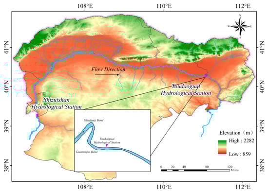
Figure 1.
Geographical location of study area.
2.2. Numerical Model
In this study, the mathematical model of river ice includes hydrodynamic model, ice dynamics model, and thermodynamic model. Based on the theory of hydraulics, thermodynamics, and river ice dynamics, the numerical simulation of river ice process under thermal-dynamic coupling is carried out [3]. The ice dynamic process, hydrodynamic process, and thermodynamic process are coupled through the interaction on the ice–water interface. Given the coupling time, based on the calibrated model parameters, the boundary conditions of hydraulic, ice, and meteorological factors are given to realize the simulation of the evolution of river ice and the process of transport and accumulation during the glacial period.
2.2.1. Governing Equation
The hydrodynamic model includes the water flow continuity equation and momentum equation.
Continuity equation:
Momentum equation:
x-direction:
y-direction:
where x, y are spatial variables, m; t is a time variable, s; H is the total water depth, m; Ht is the water depth under the ice–water interface, m; η is the height of water surface, m; qtx, qty is the component of water flow per unit width, m2/s; is the thickness of submerged ice, m; ρ is the density of water, kg/m3; , εxy is the eddy viscosity coefficient; τs is the shear stress at the ice–water interface or between the ice and free water surface, N/m2; τb is the shear stress of riverbed, N/m2.
The ice dynamics model includes surface ice motion equation, mass conservation equation, and ice concentration conservation equation.
Surface ice motion equation:
Mass conservation:
Ice concentration conservation equation:
where is the mass of ice per unit area, kg/m2; is ice density kg/m3; N is ice concentration between 0 and 100%; and the maximum density of drifting is 65% in the model. ti is ice thickness, m; is the acceleration of ice, m/s2; is the velocity of ice, m/s; is the change in surface ice area concentration caused by the mechanical accumulation of surface ice; is the drag force of wind on surface ice; and are the components of wind drag force in x and y directions, respectively; is the drag force of water flow; and are the components of the drag force of water flow in the x and y directions, respectively; and Ra is the change rate of ice concentration caused by mechanical redistribution, %/s.
The heat exchange between water surface, ice surface, and atmosphere determines the changes in water temperature, ice production, ice concentration, and ice thickness in the river during the ice period, which is the main thermal factor affecting the change in river ice [21]. The linear equation can be used to calculate the heat flux of the water surface and the ice surface. The linear expressions for calculating heat flux between the media are, respectively,
where , , is the heat exchange rate of water surface and air, ice surface and air, ice surface and water surface; is the heat exchange coefficient of air and water, ; is the average water temperature, °C; is the air temperature, °C; is a constant, generally taking 0; is the net shortwave radiation incident by the sun, which is related to the regional altitude, solar zenith angle, and solar elevation angle, ; is the heat exchange coefficient between the ice sheet surface and the air, ; is the ice surface temperature, ; is the coefficient; is the heat exchange coefficient of ice-water interface, ; and is the freezing point temperature, .
2.2.2. Initial and Boundary Conditions
The initial conditions of the model are the corresponding discharge and water level on the grid nodes. The boundary conditions include hydrodynamic, ice dynamic, and thermal-dynamic boundary conditions. The upstream boundary condition of the hydrodynamic model is the discharge, and the downstream boundary condition is the water level. The boundary conditions of the hydrodynamic model for the 2019–2020 and 2020–2021 ice periods are shown in Figure 2. The boundary conditions of the ice dynamic model include the upstream ice concentration, thickness, and size. According to the field observation, the observed ice concentration is input into the upstream boundary of the ice dynamic model. The average ice floe thickness is 0.2 m according to the field observation. The choice of ice floe size in the model is generally less than 1/15 of the river width [22]. Considering the actual field observation ice floe size and model calculation efficiency, the ice floe size is selected as 15 m in this study. The boundary conditions of the thermodynamic model of the river ice include meteorological data such as water temperature, air temperature, wind speed, and relative humidity. The daily average temperature and ice concentration during freeze-up period in 2019–2020 and 2020–2021 are shown in Figure 3.
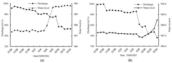
Figure 2.
Upstream flow and downstream water level during the flow and stable seal period. (a) 2019–2020; (b) 2020–2021.
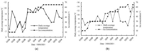
Figure 3.
Average daily temperature and ice concentration during the flow and stable seal period. (a) 2019–2020; (b) 2020–2021.
2.2.3. Model Solution and Time Step
In the governing equations of the model, the hydrodynamic equation takes into account the influence of river ice. The ice dynamics equation takes into account the influence of the internal stress, gravity, water flow, wind drag force, and river bank resistance generated by the interaction between river ice on the movement of river ice [23]. The thermodynamic equation includes the formation of surface ice, the energy exchange between the water surface and the atmosphere, the growth of border ice, and the thermal growth and regression of the ice sheet. The hydrodynamic governing equations are discretized by Euler finite element method (FEM), and the Runge–Kutta method (RKM) is used to solve the discrete equations [24]. The Lagrangian discrete particle method (DPM) is used to simulate the surface ice transport motion, and the smoothed particle hydrodynamics (SPH) method is used to solve the governing equation of ice dynamics. The internal stress between ice blocks is calculated by viscoelastic–plastic (VEP) constitutive equation [25]. The thermodynamic process is constructed by linear equations and standard heat exchange coefficients. The discretization and solution of the model governing equations are implemented through programming in VISUAL FORTRAN 6.5 software.
The time step is an important factor affecting the stability and efficiency of the model calculation. The coupling model needs to input the calculation time step of the hydrodynamic model, the calculation time step of the ice dynamic model, and the coupling time step of the two models. The criterion of time step stability is
In the formula: is the Courant number, and the size should not exceed 1; is the velocity in x direction, m/s; is the increment of time step, s; and is the grid spacing, m.
The coupling time step needs to be determined according to the simulated dynamic type. For the highly dynamic case, a smaller time interval should be used. For the slow process with thin ice thickness and hydrodynamic changes, a larger value can be used. After repeated simulation, the time step is 0.5 s, the model coupling time step is 60 s, and the ratio of the model time step to the coupling time step is 1:120. The model is stable, and the simulation efficiency is high.
3. Simulation Results and Verification
The flow of the day before the ice flow in the winter of 2019–2020 and 2020–2021 is 700 m3/s and 987 m3/s, respectively. According to the flow of the day before the ice flow, the flow and water level at each unit node of the study river section are simulated, and the initial hydraulic conditions before the ice run are obtained as shown in Figure 4. The arrows in the figure represent velocity vectors: their direction indicates the flow direction, and their length corresponds to the magnitude of the velocity. Affected by the topography and flow of the river in different years, the mainstream of the upstream river in 2019 is close to the right bank. Due to the relatively small flow, the maximum flow velocity in the upstream of the bend is less than 1 m/s. At the narrowing of the river surface at the Shisifenzi bend, the flow velocity in the river increases significantly, and the maximum flow velocity increases to 1.25 m/s. The mainstream is gradually biased towards the left bank of the river due to the influence of the bend topography. In 2020, the mainstream of the upstream river channel is in the middle of the river channel, the maximum flow velocity in the river channel is less than 1.2 m/s, and the maximum flow velocity at the narrow part of the Shisifenzi bend is increased by 1.5 m/s. The Guanniuju bend is located 6.22 km away from the upstream, and the width of the river is only 168 m, which has a significant narrowing effect on the flow. The flow velocity is symmetrical on the left and right banks, and the middle flow velocity is the largest. The downstream section of the Guanniuju bend is a straight river channel. Affected by the side bars along both banks, the main current meanders slightly within the channel; owing to the steeper downstream slope, flow velocity in this reach is somewhat higher than in the upstream section. Comparing Figure 4a,b, it can be seen that the overall flow velocity in the river channel in 2019 is less than that in 2020 due to the influence of flow rate.
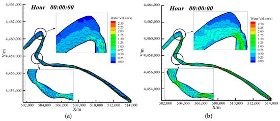
Figure 4.
Velocity distribution and velocity vector at the initial moment of ice flow. (a) 2019–2020; (b) 2020–2021.
3.1. Ice Process Numerical Simulation Under Thermal-Dynamic Coupling
Figure 5 presents the simulated distributions of river ice conditions in the Toudaoguai reach during the freeze-up period of 2019–2020 winter. In the first 24 h of the simulation, the border ice is formed in the area with low flow velocity and shallow water depth. The growth area of the border ice in the upstream of the Shisifenzi bend is larger. Under the influence of the left border ice and the mainstream bias, the surface ice floe is transported along the mainstream to the right bank side. The formation of border ice narrows the river section, weakens the ice transport capacity of the water surface, increases the ice concentration at the bend, and reduces the flow velocity. In the 48 h simulation, as ice continues to arrive from upstream, the ice concentration at the cross-section narrowed by the bend increases further, and the ice jam is formed at the narrow section of the Shisifenzi bend under the synergistic effect of border ice. After ice jamming occurred, the incoming ice from the bend’s upstream accumulated at the jam site to form an ice cover that propagated upstream. Meanwhile, the ice concentration at the constricted section near the exit of the Guanniuju bend rose sharply, creating a potential for a new jam. Both the Shisifenzi and Guanniuju bends retained an open-water reach immediately downstream of their respective jam points. By hour 72 of the simulation, ice jams had formed at both the Shisifenzi and Guanniuju bends. The area of the lead downstream of the Shisifenzi bend shrank, while the lead below the Guanniuju bend vanished as the downstream ice cover advanced, leaving almost the entire downstream channel blanketed by ice. At hour 120, as the freeze-up progressed, all remaining open-water zones within the channel disappeared, and the entire Toudaoguai reach entered duration of ice cover.
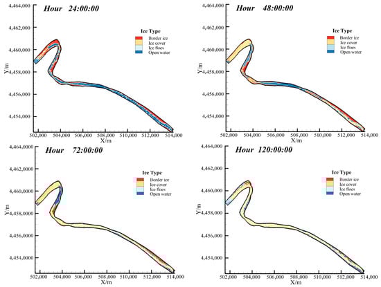
Figure 5.
Distribution of river ice morphology at different times during 2019–2020 winter.
Figure 6 shows the simulation distribution map of river ice morphology at different times in the Toudaoguai reach during freeze-up period in 2020–2021 winter. It can be seen from the map that, as in 2019–2020, border ice is first formed in the area near the river bank with shallow water depth and low flow velocity. However, due to the different river topography and inflow, the area of border ice is slightly increased compared with the previous winter. The border ice is mainly distributed near the upper and lower reaches of the Shisifenzi bend and the Guanniuju bend. At hour 48 of the simulation, some surface ice froze to the edge of the existing static border ice, forming accumulative border ice; surface ice continued to transport through the reach and no jam developed. By hour 72, border ice had extended upstream of the Shisifenzi bend, and the incoming ice flux had increased, so an ice jam first formed at this bend. The resulting ice cover propagated upstream, while the jam reduced the ice supply to the downstream reach and enlarged the area of open water. At hour 120, as the freeze-up advanced, ice jams developed at the constricted cross-sections downstream of both the Shisifenzi and Guanniuju bends and evolved into contiguous ice covers. Lead of various sizes persisted between the two jam locations. At this point the channel gradually transitioned into the stable ice-covered period.
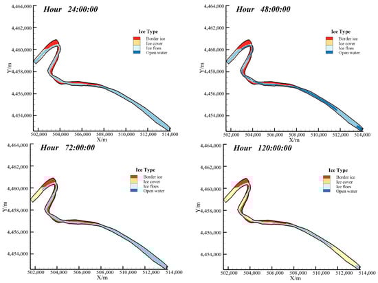
Figure 6.
Distribution of river ice morphology at different times during 2020–2021 winter.
3.2. Water Level Variation Along the Course and Validation of Simulation Result
During the freeze-up period of the winters 2019–2020 and 2020–2021, the research team conducted field observations at the Toudaoguai reach, collecting meteorological, ice, and hydrological data. The dataset includes air temperature and wind speed in the study area, ice concentration, floe size, thickness at the upstream cross-section, the ice distribution along the entire reach, ice-cover thickness at a typical section in the Shisifenzi bend, and water level at the downstream outlet section. Because of the difficult conditions during the freeze-up period, ice thickness was estimated visually by comparison; once ice cover had formed, thickness was measured by drilling holes spaced 20 m apart across the section with an L-shaped ruler.
Figure 7 shows the comparison between the simulated water level changes along the Toudaoguai reach and the measured water level at different times of the downstream Toudaoguai hydrological station in the winter of 2019–2020 and 2020–2021. It can be seen from the figure that the water level in the upstream of the Shisifenzi bend increased significantly at the 72nd hour of the simulation, but the increase in the backwater water level in 2019–2020 was less than that in 2020–2021. The change in water level depends largely on the Froude number of water flow under the condition of ice jam and is related to the ice water flow ratio and the length of ice jam [26]. As far as the flow structure is concerned, the flow field shape of the curved channel is significantly different from that of the straight channel due to the existence of spiral flow. The flow velocity and Froude number in the curved channel are significantly smaller than those in the straight channel, and the ice water level increment is smaller than that in the straight channel. In 2019, the ice accumulation at the Shisifenzi bend showed a wedge-shaped shape from the convex bank to the concave bank, and the mainstream was biased towards the non-ice jam area of the concave bank. In 2020, the ice accumulation in the upstream river channel of the Shisifenzi bend kept the two sides flat and developed upstream, and the ice flow along the straight river channel accumulated to the entire river section. Therefore, the Increase in ice water level in 2019 was less than that in 2020. At the same time, the simulated water level of Toudaoguai hydrological station at different times is compared with the measured water level, and the two are in good agreement. Figure 8 shows the comparison between the measured ice thickness and the simulated value of the typical section at the Shisifenzi bend. Affected by the topography, the mainstream of the section is close to the convex (right) bank side of the bend, and the erosion effect of the water flow on the bottom of the ice sheet is significantly greater than that of the concave (left) bank, resulting in the ice thickness on the right side of the river section is smaller than that on the left bank side. Due to the limited number of observed water level data, no validation metrics between modeled and measured water levels were calculated. Based on the simulated and observed ice thickness, the RMSEs computed for the 2019–2020 and 2020–2021 winter periods are 0.032 and 0.009, respectively, and the NSEs are 0.898 and 0.976.

Figure 7.
The variation in simulated water level along the river and the comparison between riverbed elevation and measured water level. (a) 2019–2020; (b) 2020–2021.
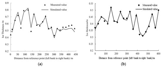
Figure 8.
Comparison of simulated ice thickness and measured ice thickness in Shisifenzi bend. (a) 2019–2020; (b) 2020–2021.
Therefore, the accuracy of the mathematical model is verified by comparing the simulated water level change and ice thickness with the measured values, indicating that the mathematical model can accurately simulate the hydraulic characteristics and river closure process of natural rivers.
4. Discussion on Key Parameters of the Model and Sensitivity Analysis
The river ice process is a complex physical phenomenon governed by the interplay of thermal, hydrodynamic, and ice-dynamic forces. When modeling this process, one must not only calibrate the bed and ice-cover roughness coefficients but also specify several critical parameters for the hydrodynamic, ice-dynamic, and thermal sub-models. Because the appropriate values of these parameters vary with boundary conditions, climatic characteristics, and the specific features of the river ice regime, their proper selection is essential to the accuracy and reliability of the simulation results.
4.1. Hydrodynamic Parameter
In the hydrodynamic simulation, the dry–wet boundary method is used to deal with the intertidal zone. The value of dry depth and wet depth in the dry–wet boundary method will have an important impact on the stability and accuracy of the model. For a given calculation time step, if the minimum depth value is too large, the calculation accuracy will be affected, and if the value is too small, the calculation will be unstable. Therefore, setting the appropriate minimum depth can not only ensure the stability of the model calculation but also ensure the accuracy of the calculation results. In the simulation, the parameters are set to 0.5 m, 0.2 m, and 0.1 m, respectively. The simulation results under different settings are analyzed. When the minimum depth is set to 0.1 m, the model simulation is unstable, and the calculation results are divergent. When it is set to 0.5 m or 0.2 m, the hydrodynamic simulation remains stable; however, because a lower value yields higher accuracy, the parameter is ultimately fixed at 0.2 m.
4.2. Border Ice Parameters
The formation of border ice will significantly affect the width of river ice transport, which has an important influence on the formation of initial ice jam. The parameters of border ice formation mainly include the critical water surface temperature of border ice formation , the critical flow rate of static border ice , the critical flow rate of alluvial border ice , and the maximum density of border ice formation . Among them, the critical velocity of static border ice directly affects the formation range and area of border ice. When Li Chao simulated the Sanhuhekou reach of the Yellow River (Inner Mongolia reach), the critical velocity of static border ice was 0.25 m/s [27], but when the parameter value was applied to the Shisifenzi reach, the simulation results showed that the border ice formation area at the bend did not match the field photos as shown in Figure 9. Based on the field observation of Matousek, it is pointed out that the static border ice stops lateral growth when the value is greater than 0.40 m/s [28]. In this paper, the critical velocity of static border ice is set to 0.25 m/s, and 0.35 m/s, respectively, for simulation. It can be seen that when = 0.35 m/s, the position and range of simulated border ice in Figure 10 are in good agreement with the observation results. At this time, border ice is formed at the concave bank of the upstream Shisifenzi bend and the convex bank of Guanniuju bend, and the width of border ice occupies 3/4 of the river width. Therefore, the critical velocity of forming static border ice is determined to be 0.35 m/s.
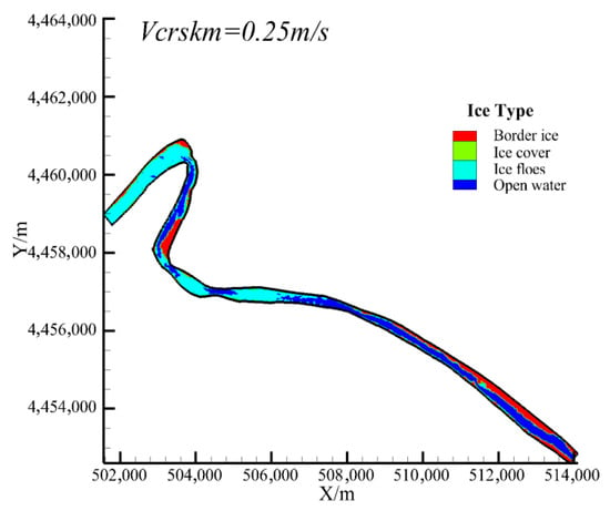
Figure 9.
Distribution of river ice morphology at critical velocity = 0.25 m/s.
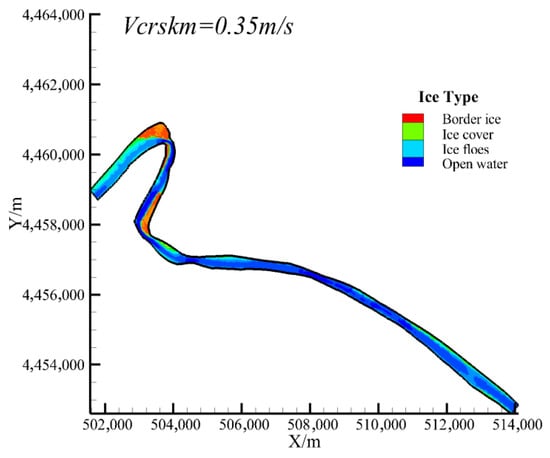
Figure 10.
Distribution of river ice morphology at critical velocity = 0.35 m/s.
4.3. Heat Exchange Coefficient
The heat exchange coefficient in the model affects the ice production and ice-cover thickness of the river, and the heat exchange coefficient in this area can be calculated more accurately by using the linearized equation. Figure 11 shows the changes in daily average shortwave radiation and longwave radiation in the study area in 2019 and 2020, respectively. The net short-wave radiation is substituted into the linear equations of heat flux (7) and (8), where takes 0, , , and refer to the reference value of Shen in the same latitude area, and the heat exchange coefficients of Toudaoguai reach are calculated as = 21.38 , = 15 , and = 32.574 .
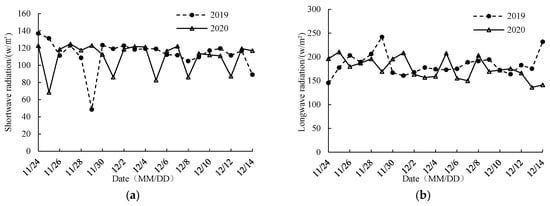
Figure 11.
Changes in shortwave radiation and longwave radiation in Toudaoguai hydrological station during the ice-stable period in 2019 and 2020. (a) Shortwave radiation; (b) longwave radiation.
Based on the Shen & Chiang nonlinear thermodynamic model and combined with a linear thermodynamic approach, Zhao et al. [29] calibrated the heat-loss coefficient for the Inner Mongolia reach of the Yellow River during the ice-covered period, and their result is close to that obtained in this study. Referencing areas in the United States at the same latitude, for example, Lal and Shen [30] took 19.7 in the northern river of the United States, and Blackburn and Shen [31] took 20 in the Susitna River of Alaska, United States. Finally, it is determined that the water surface–atmosphere heat exchange coefficient between 39° and 42° north latitude is 21.38 during the freeze-up period.
The selection of some parameters in the model needs to consider the actual situation of the study area and be calibrated with the measured data. The key parameters of the numerical simulation of the river ice process in the Toudaoguai reach of the Yellow River are given in Table 1.

Table 1.
Key parameters of river water–ice thermal coupling model.
4.4. Parameter Sensitivity Analysis
The freeze-up process of natural rivers is a complex physical process coupled with hydraulic, ice, river, and meteorological factors. According to the process of river closure in 2019–2020 and 2020–2021, there are great differences in the form and process of river closure due to the different influencing factors of freeze-up. In order to explore the key factors in the process of freeze-up in this study, eight model parameters such as discharge Q, water level Z, ice concentration N, ice-cover roughness coefficient , riverbed roughness coefficient , critical velocity of border ice non-accumulation , critical Froude number , and ice porosity were selected. The modified Morris screening method was used to analyze the key parameters affecting freeze-up [32]. This approach is a “simplified-fixed-step” variant of the classical Morris method tailored for engineering practice. While preserving the one-at-a-time philosophy, it replaces the original random discrete steps with percentage-based increments, yielding controllable perturbation sizes and more intuitive operation; sensitivity is then assessed directly through the ratio of relative change rates.
The modified Morris screening method is to keep other parameter values and boundary conditions unchanged and increase a certain parameter by a certain proportion in a single time. By comparing the changes in the backwater water level after ice jam, the sensitivity of the parameter is analyzed. Figure 12 shows the results of the modified Morris screening method for each parameter in 2019–2020 and 2020–2021. It can be seen that the discharge Q and the ice concentration N are the most sensitive to the change in the backwater water level after the ice jam, and the sensitivity is more than 50%. It shows that the upstream flow and the amount of ice in the ice period have the greatest influence on the frozen river in the river channel. The increase of flow not only directly leads to the increase in river water level but also causes the mechanical thickening of the ice-cover. An increase in ice volume raises the likelihood of river channel ice jam formation, which can in turn trigger more severe ice blockages and cause upstream water levels to rise. At the same time, the ice-cover roughness coefficient and the ice porosity are more sensitive coefficients. The sensitivity of the ice-cover roughness coefficient ni in 2020–2021 reaches 22%, which is higher than the sensitivity of the ice cover roughness coefficient ni in 2019–2020. The main reason was that during the winter of 2020–2021, the upstream shore ice in the Shisimazi bend grew so extensively that it severely narrowed the river’s ice-transport cross-section, causing the channel to freeze over; once the ice cover formed, its increased roughness raised flow resistance and pushed upstream water levels higher. The sensitivity of ice porosity is negative, indicating that the larger the porosity of ice accumulation, the lower the water level at the time of river frozen. The riverbed roughness coefficient and the water level Z are low sensitive parameters, and the critical velocity and the critical Froude number do not affect the water level change, which are non-sensitive parameters.
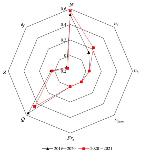
Figure 12.
Analysis results of modified Morris method in 2019–2020 and 2020–2021.
To further analyze how the highly sensitive factors—ice concentration N and discharge Q—affect water-level variations at the Toudaoguai reach during the stable ice-covered period. Figure 13 and Figure 14 give the relationship between the flow ice concentration N and discharge Q in the upstream channel of the Shisifenzi bend and the relative increment of water level in freeze-up period ΔH/H0, where ΔH is the increase in cross-sectional water level during the ice period, and H0 is the water depth without ice. It can be seen from Figure 13 that the ice concentration N and the relative increment of water level in the freeze-up period show a linear growth relationship of ΔH/H0, while the relative increment of water level in the freeze-up period increases first and then decreases with the increase in upstream flow, and the discharge corresponding to the maximum increment of water level in different years is inconsistent. The discharge at the maximum increment of water level in the freeze-up period from 2019 to 2020 is 730 m3/s, and the discharge at the maximum increment of water level in winter from 2020 to 2021 is 370 m3/s. The increase in water level is mainly affected by the increase in discharge and the accumulation of ice [33]. The increase in discharge has a relatively stable influence on the rise in water level, while the accumulation of ice has a great influence on the rise in water level, which is the reason why the relative increment of water level has a peak value (as shown Figure 14). The growth mode of ice cover in the studied river section is hydraulic thickening and mechanical thickening. When the discharge is small, the ice cover is hydraulic thickening, and the backwater effect of the water level channel is not obvious. When the flow rate increases, the mechanical thickening mode of the ice cover begins to occur. After a large amount of flowing ice accumulates into ice jams under mechanical action, the water level of the river channel is obviously raised, and the relative increment peak of the water level appears. However, with the further increase in flow rate, the hydraulic effect is further strengthened, resulting in the accumulation of ice at the bottom of the ice cover gradually being eroded away, the backwater phenomenon gradually weakened, and the relative increment of water level decreased. Therefore, the relationship between the upstream discharge Q and the relative increment of water level in the freeze-up period ΔH/H0 increases first and then decreases. The discharge corresponding to the relative increment peak of water level in different years is different, which needs to be further discussed according to the factors such as ice form and the ice jam location in the year.
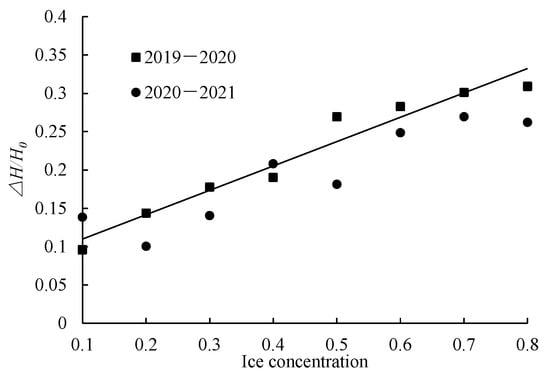
Figure 13.
The relationship between the stream density N and ΔH/H0.
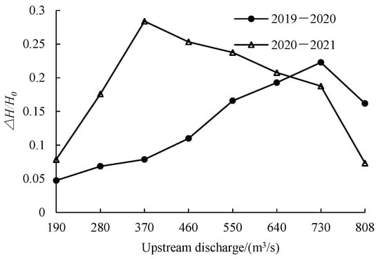
Figure 14.
The relationship between upstream discharge Q and ΔH/H0.
5. Conclusions
In this paper, based on the two-dimensional hydrodynamic model and ice dynamics model, coupled with the linear thermodynamic process, the Toudaoguai reach of the Inner Mongolia reach of the Yellow River is taken as an example to simulate the river ice transport and accumulation process in the winter of 2019–2020 and 2020–2021. The simulation results are compared with the measured data, and the key parameters of the model are discussed. The sensitivity of the water level change and its sensitivity after the freeze-up are discussed. The following conclusions are obtained: (1) The mathematical model can well simulate the hydraulic characteristics, ice thickness growth, and freeze-up morphology of natural rivers. (2) The values of model parameters in different study areas are different. The dry–wet boundary conversion of Toudaoguai reach is 0.2 m, the critical velocity of static border ice is 0.35 m/s, and the water–air–heat exchange coefficient is 21.38 . (3) The discharger Q and the ice concentration N are the most sensitive to the change in the backwater level of the ice jam. The relative water level increment has a linear relationship with the ice concentration and increases first and then decreases with the increase in the discharge.
Therefore, in natural rivers the size of ice floes varies widely and ice concentration changes dynamically with time; both factors are critical to the morphology, location, and timing of ice-cover formation. In the present model, however, all ice floes are assigned a uniform size, and their density is prescribed from manual observations whose accuracy is limited by the measurement technique, potentially degrading simulation fidelity. Future work could employ semantic-segmentation models to automatically identify floe size and density and couple this capability with the river ice model to improve predictive skill. Moreover, because the current ice model is formulated within a continuum framework, subsequent studies could incorporate the discrete element method to elucidate the micro-mechanisms governing ice jam initiation.
Author Contributions
Conceptualization, C.L. and L.M.; methodology, L.M. and C.L.; software, X.J.; validation, L.M., C.L. and X.J.; investigation, Z.Y.; data curation, Z.Y.; writing—original draft preparation, L.M., X.J. and C.L.; writing—review and editing, C.L. and L.M.; supervision, Z.Y.; funding acquisition, C.L. and Z.Y. All authors have read and agreed to the published version of the manuscript.
Funding
This research was funded by the National Natural Science Foundation of China—Yellow River Water Science Joint Fund (grant No. U2443205), the Inner Mongolia Autonomous Region Science and Technology Plan Project (grant No. 2023YFSH0002), the Natural Foundation of Inner Mongolia (grant No. 2023MS05023), the Central Government Guided Local Science and Technology Development Fund Project (grant No. 2024ZY0065), and the Basic Scientific Research Business Fee of Directly affiliated Universities in Inner Mongolia Autonomous Region (grant No. BR231516).
Data Availability Statement
Datasets including Runoff and Sediment load were derived from public domain resources.
Acknowledgments
Acknowledgements are extended to the State Key Laboratory of Water Engineering Ecology and Environment in Arid Area, Inner Mongolia Agricultural University for their financial support of this research paper.
Conflicts of Interest
The authors declare no conflicts of interest.
References
- Beltaos, S. Hydraulics of Ice-Covered Rivers. In Issues and Directions in Hydraulics; Nakato, T., Ettema, R., Eds.; Balkema: Rotterdam, The Netherlands, 1996. [Google Scholar] [CrossRef][Green Version]
- Ze, Y.M.; Jian, J.W.; Yun, T.S. River Ice Processes. J. Hydroelectr. Eng. 2002, 153–161. [Google Scholar] [CrossRef]
- Shen, H.T. Mathematical modeling of river ice processes. Cold Reg. Sci. Technol. 2010, 62, 3–13. [Google Scholar] [CrossRef]
- Shen, H.T.; Chiang, L. Simulation of growth and decay of river ice cover. J. Hydraul. Eng. 1984, 110, 958–971. [Google Scholar] [CrossRef]
- Ashton, G.D. Deterioration of floating ice covers. J. Energy Resour. Technol. 1985, 107, 177–182. [Google Scholar] [CrossRef]
- Shen, H.T.; Su, J.; Liu, L. SPH Simulation of River Ice Dynamics. J. Comput. Phys. 2000, 165, 752–770. [Google Scholar] [CrossRef]
- Shen, H.T.; Lu, S. Dynamics of River Ice Jam Release. In Cold Regions Engineering: The Cold Regions Infrastructure—An International Imperative for the 21st Century; ASCE: Reston, VA, USA, 2010. [Google Scholar]
- Knack, I.M.; Huang, F.; Shen, H.T. A Numerical Model Study on St. Marys River Ice Conditions. In Proceedings of the 21st IAHR International Symposium on Ice, Dalian, China, 11–15 June 2012. [Google Scholar]
- Huang, F.; Shen, H.T.; Knack, I. Modeling Border Ice Formation and Cover Progression in Rivers. In Proceedings of the 21st IAHR International Symposium on Ice, Dalian, China, 11–15 June 2012. [Google Scholar]
- Wazney, L.; Clark, S.P.; Malenchak, J.; Knack, I.; Shen, H.T. Numerical simulation of river ice cover formation and consolidation at freeze-up. Cold Reg. Sci. Technol. 2019, 168, 102884. [Google Scholar] [CrossRef]
- Xu, G.B. One-dimensional mathematical models of river ice evolving process. J. Water Resour. Water Eng. 2011, 22, 78–83+87. [Google Scholar] [CrossRef]
- Ke, S.; Zhang, X.; Wang, Y. Research on Prediction Mathematical Model of Freeze-up of River Ice Cover. J. Glaciol. Geocryol. 2001, 23, 328–332. [Google Scholar] [CrossRef]
- Yang, K. Heat exchange model between river-lake and atmosphere during ice age. J. Hydraul. Eng. 2021, 52, 556–564+577. [Google Scholar] [CrossRef]
- Yang, K. Water temperature models of open channels in glacial period. J. Hydraul. Eng. 2022, 53, 20–30. [Google Scholar] [CrossRef]
- Zhai, B.; Liu, L.; Shen, H.T.; Ji, S. A numerical model for river ice dynamics based on discrete element method. J. Hydraul. Res. 2022, 60, 543–556. [Google Scholar] [CrossRef]
- Zhai, B.; Shen, H.T.; Liu, L.; Pan, J.; Jia, D. DEM simulation of wave-generated river ice cover breakup. Cold Reg. Sci. Technol. 2024, 218, 104084. [Google Scholar] [CrossRef]
- Luo, H.C.; Ji, H.L.; Gao, G.M.; Zhang, B.S.; Mou, X.Y. Study on the characteristics of flow and ice jam formation in Shisifenzi bend in the Yellow River during the freeze-up period. J. Hydraul. Eng. 2020, 51, 1089–1100. [Google Scholar] [CrossRef]
- Zhao, S.; Li, C.; Li, C.; Shi, X.; Zhao, S. Processes of river ice and ice-jam formation in Shensifenzi Bend of the Yellow River. J. Hydraul. Eng. 2017, 48, 351–358. [Google Scholar] [CrossRef]
- Li, M.K.; Ji, H.L.; Mou, X.Y.; Zhang, B.S. Effects of ice cover on flow and sediment characteristics of the Shisifenzi reach in the Yellow River. J. Sediment. Res. 2021, 46, 23–29. [Google Scholar] [CrossRef]
- Sun, B.; Zhou, R.; Wang, Z.; Xiao, J.; Ma, J.; Li, C.; Ma, B. The simulation study of wind erosion characteristics of different soils in Inner Mongolia reach of Yellow River. J. Desert Res. 2020, 40, 120–127. [Google Scholar] [CrossRef]
- Zhao, S.; Chen, X.; Wang, W.; Zhou, Q.; Yin, H.; Li, W. Nonlinear thermodynamic analysis of water surface-atmosphere during freeze-up period of the Inner Mongolia reach of the Yellow River. J. Water Resour. Water Eng. 2021, 32, 130–136. [Google Scholar] [CrossRef]
- Shen, H.T.; Lu, S.; Crissman, R.D. Numerical simulation of ice transport over the Lake Erie-Niagara River ice boom. Cold Reg. Sci. Technol. 1997, 26, 17–33. [Google Scholar] [CrossRef]
- Connor, J.J.; Brebbia, C.A. Finite Element Techniques for Fluid Flow; Newnes: Oxford, UK, 2013. [Google Scholar] [CrossRef]
- Li, C.; Li, C.; Shen, H.T. Characteristics of surface ice movement in a channel bend with intake and the layout of ice deflection booms. Adv. Water Sci. 2014, 25, 233–238. [Google Scholar] [CrossRef]
- Shen, H.T.; Gao, L.; Kolerski, T.; Liu, L. Dynamics of ice jam formation and release. J. Coast. Res. 2008, 10052, 25–32. [Google Scholar] [CrossRef]
- Sui, J.; Karney, B.W.; Fang, D. Variation in water level under ice-jammed condition—Field investigation and experimental study. Hydrol. Res. 2005, 36, 65–84. [Google Scholar] [CrossRef]
- Chao, L. Study on Characteristics of River Ice Evolution and Numerical Simulation of the Yellow River (Inner Mongolia Reach). Ph.D. Thesis, Inner Mongolia Agricultural University, Hohhot, China, 2015. [Google Scholar]
- Michel, B.; Marcotte, N.; Fonseca, F.; Rivard, G. Formation of border ice in the St. Anne River. In Proceedings of the 2nd CRIPE Workshop, Edmonton, AB, Canada, 6–9 June 1982; pp. 38–61. [Google Scholar]
- Zhao, S.; Shen, H.T.; Shi, X.; Li, C.; Li, C.; Zhao, S. Winter time surface heat exchange for the Inner Mongolia reach of the Yellow River. J. Am. Water Resour. Assoc. 2020, 56, 348–356. [Google Scholar] [CrossRef]
- Lal, A.W.; Shen, H.T. A Mathematical model for river ice processes. J. Hydraul. Eng. 1991, 117, 851–867. [Google Scholar] [CrossRef]
- Blackburn, J.; She, Y. A comprehensive public-domain river ice process model and its application to a complex natural river. Cold Reg. Sci. Technol. 2019, 163, 44–58. [Google Scholar] [CrossRef]
- Ru, T.L.; Zong, X.X.; Chen, L.Y. Parameter sensitivity analysis methods of Storm Water Management Model. J. Hydroelectr. Eng. 2022, 41, 11–21. [Google Scholar] [CrossRef]
- Tao, W.; Pang, P.C.; Shu, Y.L.; Wang, J. Experimental study of critical condition of ice jam formation in a curved channel. South-to-North Water Transf. Water Sci. Technol. 2016, 14, 87–90. [Google Scholar] [CrossRef]


Disclaimer/Publisher’s Note: The statements, opinions and data contained in all publications are solely those of the individual author(s) and contributor(s) and not of MDPI and/or the editor(s). MDPI and/or the editor(s) disclaim responsibility for any injury to people or property resulting from any ideas, methods, instructions or products referred to in the content. |
© 2026 by the authors. Licensee MDPI, Basel, Switzerland. This article is an open access article distributed under the terms and conditions of the Creative Commons Attribution (CC BY) license.