Modeling and Assessment of Salinity Reduction Strategies in the Jarahi River, Iran

Abstract

This study investigates the spatial and temporal variations in salinity in the Jarahi River and its traditional channels using field measurements and numerical simulations. The primary objective is to assess the effectiveness of different management strategies for salinity reduction under minimum-discharge conditions. Salinity dynamics were analyzed through electrical conductivity (EC) measurements collected over a one-year period and simulated using the MIKE 11 hydrodynamic model. Model performance was evaluated by comparing simulated and observed EC values at key monitoring stations. The results indicate that maximum salinity levels occur during March and April in both the main river and traditional channels, while the highest temporal variability in EC was observed in October. The comparison between observed and simulated data showed a relative error of less than 10%, confirming the reliability of the model simulations. Four management scenarios were evaluated: (1) preventing inflow from the Motbeg drainage, (2) blocking non-centralized drainage inputs, (3) removing all inlet drains, and (4) increasing discharge releases from the Ramshir Dam. The first and third scenarios led to the highest salinity reductions, reaching up to 39% (approximately 1266 µS/cm) in the Gorgor channel, while reductions of up to 53% were observed in traditional streams such as Mansuri and Omal-Sakher under the third scenario. Increasing dam releases resulted in a maximum reduction of 23% (724 µS/cm) at the Gorgor station. Finally, the proposed management strategies significantly reduced salinity levels along the river system, particularly at the entrance of the Jahangiri traditional stream, providing practical insights for salinity control and river basin management.

1. Introduction

Although about 70% of the Earth’s surface is covered by water, approximately 97.5% of this amount is saline, and only 2.5% is freshwater. Of this limited freshwater fraction, less than 1%, most of which is stored in rivers, lakes, and shallow groundwater, is accessible for human use [1]. This limited availability has made freshwater resources increasingly vulnerable to both quantitative scarcity and quality degradation worldwide. The scarcity of freshwater alone represents a significant challenge. In addition, factors such as population growth, climate variability, indiscriminate water extraction, and droughts have further intensified these challenges, as a result, reduced access to freshwater has emerged as a major social, agricultural, public health, and food security concern in many regions [2]. Moreover, floods and sediment laden flows have further exacerbated the reduction in access to safe and reliable water sources [3,4]. Therefore, in addition to the availability of water, water quality is another critical factor that must be considered in the process of supplying water for agriculture and other activities [5]. Various factors, such as the entry of sewage and salinity into water sources like rivers, cause changes in the quality parameters of river water, ultimately reducing its suitability for use [6,7,8]. One of the key parameters for assessing river water quality is salinity [9]. Salinity indicates the concentration of dissolved salts in water [10]. An increase in salinity directly affects the mortality and behavior of aquatic animals, damages coastal ecosystems, and reduces water quality for agricultural, domestic, and commercial use [11]. Mohammadzadeh-Habili et al. [12] highlighted that both natural geogenic factors and human interventions contribute significantly to increased salinity levels, particularly during periods of low discharge. This underscores the need for integrated management strategies to mitigate salinity in vulnerable river systems. Therefore, measuring salinity in rivers is crucial to understanding current conditions, evaluating different scenarios, and developing solutions for mitigating, reducing, and controlling salinity and its destructive effects [13]. The following section provides an overview of several studies conducted on river salinity.

Changes in water levels due to salinity have been a significant focus of research. Bhuiyan and Dutta [14] investigated the effects of salinity on water levels in the Gorai River in 2002. The results showed that a sea level rise of 59 cm led to a salinity change of 0.9 at 80 km upstream of the river mouth, corresponding to a climatic effect of 1.5 per meter of sea level rise in the Gorai River. Rice et al. [15] used a calibrated three-dimensional model to simulate salinity changes in the James and CHK Rivers caused by sea-level rise. In addition to the general finding that salinity increases throughout the river with rising water levels, they specifically noted that salinity is higher in dry years than in wet years. Xiao et al. [16] studied the effects of sea level rise on salinity intrusion in the St. Mark River estuary using a 3D hydrodynamic model. Under a sea level rise of 0.85 m, numerical modeling for the 4 months in 2000 indicated that the sea level rise could cause a significant increase in salinity near the lower Wakulla River, with an increase of 9.2 for surface salinity and 12.7 for bottom salinity. Additionally, they also investigated the salinity of the tidal river. Uncles and Stephens [17] reported that salinity intrusion into the freshwater reach occurs due to tidal changes. Salinity intrusion occurs not only during spring tides but also during intermediate and neap tides. The amount of salinity and the extent of salinity intrusion vary with the different types: spring, intermediate, and neap tides. Vale and Dias [18] investigated the salinity of the Lima tidal river using a numerical model based on the minimum and average discharge of the river. Koutsoyiannis [19] mentioned that the sea-level rise can cause an increase in salinity, but the overexploitation of water resources can also cause the sea-level and salinity to increase. Qureshi et al. [20] underlined integrated management strategies, including soil amendments, saline water utilization, and salt-tolerant crop selection, as key solutions for salinity challenges in Iran. Such approaches aim to rehabilitate degraded lands while ensuring sustainable agricultural productivity. Other studies, such as those by Adib and Javdan [21], Siles-Ajamil et al. [22], Farahani et al. [23], and Matsoukis et al. [24], also focused on salinity in tidal rivers.

The relationship between discharge and salinity is an important factor in understanding salinity in rivers. Zhang et al. [25] measured salt infiltration and the extent of salt intrusion at the river mouth through numerical studies. Jeong et al. [26] analyzed the properties of salinity infiltration in the lower reaches of the Geom River using a three-dimensional numerical model based on the Environmental Fluid Dynamics Code (EFDC). Their research outcomes showed that the EFDC model used for numerical simulation is highly accurate, and the results obtained can serve as a foundation for understanding the effects of salinity infiltration at varying discharges. Meanwhile, Al-Thamiry and Haider [27] investigated salinity and the relationship between salinity and discharge in the Euphrates River using the HEC-RAS v.4.1 mathematical model. To estimate the peak flood discharge with different return periods using probability distribution functions, selecting an appropriate distribution is of great importance. Dimitriadis et al. [28] fitted streamflow data to the truncated-mixed PBF distribution, considering its skewness–kurtosis diagram limitations, to assess whether it can adequately simulate the observed values estimated through the K-moments by including a nonzero probability at a lower truncation point. They found that although similarities were observed in the skewness–kurtosis diagram, the stronger estimation of L-skewness versus L-kurtosis allows for a more robust comparison. However, more advanced estimations of K-skewness and K-kurtosis provide a clearer view of the identified pattern.

Finally, all the reviewed studies indicate that salinization of rivers has now turned into one of the most pressing current environmental and water management concerns linked to sea-level rise, reduced river discharge, and variations in tidal dynamics, further exacerbated by human pressures such as overextraction of water and agricultural return flows. The magnitude of salinity intrusion reported across different basins shows a clear time and increasing trend; some studies showed that the intensity of salinity increases, especially in low flow periods and dry years, with rising sea levels significantly enhancing the inland movement of saline waters. Numerical investigations based on hydrodynamic modeling frameworks, including EFDC, HEC-RAS, and MIKE-based models, consistently identify river discharge as a key controlling factor governing both the extent and severity of salinity intrusion. The literature also emphasizes unmanaged salinity growth leading to serious ecological and agricultural impacts through fresh-water habitat degradation, reductions in crop productivity, and long-run declines in soil and water quality. It also emphasizes the necessity for integrated salinity management strategies, as suggested earlier, which consider changing reservoir releases, regulating drainage inputs, improved agricultural practices, and the employment of techniques of soil and crop management. Overall, the convergence of findings from earlier research underlines the need to address salinization and the importance of detailed and model-supported planning in preventing its advance in sensitive river systems.

In the current research, both field measurements and numerical modeling were carried out, along with the implementation of different scenarios, to investigate salinity in the Jarahi River. Field observations combined with MIKE 11 software were applied to analyze salinity variations and its associated traditional streams, focusing particularly on the minimum discharges during different months/seasons of the year. The study also aimed to identify practical solutions for controlling and reducing salinity in the river and its tributary channels. Furthermore, EC levels were comprehensively examined throughout various months to assess seasonal changes.

2. Materials and Methods

2.1. Case Study

The current research was conducted through the Jarahi River in Iran, as shown in Figure 1. The length of the Jarahi River from the confluence of the two rivers, Allah and Marun, to its mouth in Khur Musa is 210 km, and from the source of the Marun River to the mouth is 520 km [29]. It is estimated that the watershed area is about 23,245 km², of which about 10,910 km² is mountainous and the remaining 12,325 km² are plains and foothills. The remaining 12,325 km² are plains and foothills [29]. The Jarahi River, which passes through the fertile plain of Khuzestan province, is an important water supply source for use in various sectors of agriculture, industry, urban development, and fish farming. All of these have caused the discharge to decrease by water harvesting [30].

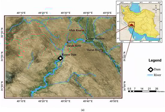
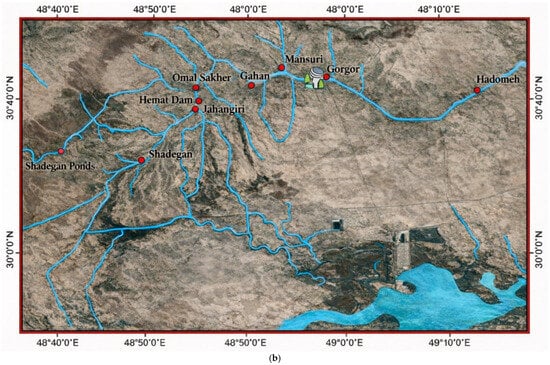
Figure 1. (a) A view of the Jarahi River, the border between the Allah and Marun Rivers; (b) view of the investigated area with inlet streams and side information.

In the area between Ramshir Dam and Shadegan Wetland, five relatively large channels branch off from the Jarahi River, each of which turns out water from this River (Figure 1b). The first branch is the Gorgor channel, which is located about 108 km from the Ramshir dam and turns out at the right bank of the Jarahi river. The second one is Mansuri, situated about 117 km from Ramshir Dam, and this channel branches off from the right bank of the Jarahi River. The third one is the Gahan channel, situated about 123 km from the beginning of the study reach and branches off from the left bank of the Jarahi River. The next channel is Omal Sakher, located 140 km from the Ramshir Dam and turns out from the Jarahi right bank. Jahangiri channel after Hemat and Pumping Station Dam are on the river at about 142 km from Ramshir Dam, from the left bank of the river [31,32]. It should be mentioned that Hemat and Pumping Station Dam has a hydrometry station known as Shadegan hydrometric station, located about 141 km from Ramshir Dam. The most critical drain in the region that brings agricultural pollutants into the Jarahi River is a drain named Motbeg with coordinates of latitude 343228 and longitude 3410478. Such a water system with three channels and branch flow is considered in terms of the technical points required in river modeling, as shown in Figure 1b.

2.2. Field Data Surveying and Collection

In the first step, a map survey was conducted within reach of the river between Ramshir Dam and Shadegan Wetland. Taking cross-sections of the Jarahi River in this reach, cross-sections of the mentioned branched or turned-out channels, and transferring the height code from sea level to zero points of the water level measurement stations were the things in this section. The WILD NA2 leveling mapping camera (Wild Heerbrugg, Heerbrugg, Switzerland), an STS-752R total station (China), and a Garmin handheld GPS (Garmin Ltd., Olathe, Kansas, USA) were used to carry out the mapping [33]. The round-trip alignment method transferred the code from the Benchmark (BM) of the National Cartographic Centre (NCC) of Iran [34]. The total station camera was used to transfer flat coordinates in the UTM system [34]. Then, the height and flatness of the base were measured according to the available BM in the area. The height and plane coordinates of 17 mapping stations of the studied area available in the Khuzestan Water and Power Authority (KWPA) sources were used in this operation. Generally, 24 cross-sections were surveyed from the Jarahi River every 10 km to map cross-sections from Ramshir Dam and Shadegan Wetland, where the names of the sections are JA1 to JA24, respectively. Figure 2 shows the data collection activities for the current research. In addition, the sections were taken from 100 to 200 m upstream and downstream of the river’s branching channels. In addition, the cross-sections were measured from the flow path in the Ramshir Dam area to the Shadegan Wetland. The list of channels that were measured in the cross-sections is given in Table 1. Finally, the zero-elevation code of the river water level gauging stations was measured, including the Abu tavij, Gorgor, Shahid Hemmat Dam, and Khorosi stations.

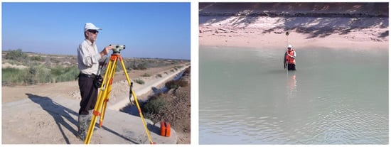
Figure 2. Examples of field surveying activities illustrate topographic mapping and spatial data collection along the river and traditional channels.

Table 1. Hydrometric stations of the Jarahi River within the project reach.

Number	Hydrometry Station	Easting	Northing	Height to Sea Level
1	Abu Tavij	0.02	0.185	4.03
2	Gorgor	0.016	0.185	6.30
3	Shahid Hemmat Dam	0.013	0.185	9.54
4	Khorosi-Shadegan	0.02	0.185	2.27

2.3. Discharge Measurement in the Jarahi Rivers and Traditional Channels

The discharge of the Jarahi River and its branches (from Ramshir Dam to Shadegan Wetland reach) for each cross-section upstream of each branched river in the year’s four seasons namely, spring, summer, fall, and winter, was measured. Initially, 16 stations were selected to record changes in discharges, and their geographic coordinates were determined on aerial maps. In each measurement, the position of the river water side was considered the origin, which was recorded by the GPS device [35]. Then, it was necessary to survey the river width every 10 m according to the information input to the device. This length was determined according to the wind and flow velocity in the river as it caused the boat not to settle at the desired point. For this reason, GPS and anchors were used to control and reduce errors and position the boat at any distance. Then, the GPS position was set, and the flow measuring device was placed in the flow after the boat was placed at any vertical point [35]. Then, Qlinear recorded the depth and velocity of the flow simultaneously. Finally, the river flow and bed profile were extracted after completing the survey in each measurement. It is necessary to explain that this process was performed by Qlinear software after transferring the measured data. This software calculates the velocity and depth of flow and the bed profile in open channels. Table 2 reports the measured discharge values in different seasons at the measurement location.

Table 2. The Measured Discharge at Different Locations.

No.	Location	Discharge ($\raisebox{1ex}{${\mathbf{m}}^3$}\!\left/ \!\raisebox{-1ex}{$\mathbf{s}$}\right.$)
		December 2019	March 2020	May 2020
1	Jarahi River (before the intersection of Jarahi River with Gorgor Channel)	33.98	17.56	18.9
2	Gorgor channel (entrance from Jarahi river to Gorgor Channel)	0	0	0
3	Jarahi River (before the intersection of Jarahi River with Mansuri Channel)	30.15	14.98	18.1
4	Mansuri Channel (entrance from Jarahi River to Mansuri Channel)	0	0	0
5	Jarahi River (before the intersection of Jarahi River with Omal Sakher Channel)	28.2	13.72	17.6
6	Gahan Channel (entrance from Jarahi River to Gahan Channel)	0	0	0
7	Jarahi River (before the intersection of Jarahi River with Omal Sakher Channel)	25.02	1028	15.4
8	Omal Sakher Channel (entrance from Jarahi River to Omal Sakher Channel)	0	0	0
9	Jarahi River (before the water intake of Hemat Pumping Station)	23.83	9.722	13.7
10	Jarahi River (after the intersection of Jarahi River with Jahangiri Channel)	11.186	4.852	8.2
11	Jahangiri Channel (entrance from Jarahi River to Jahangiri Channel)	3.5	1.2	3
12	Jarahi River (before the intersection of Jarahi River with Topchi, Mandvan, and Abshar Channel)	14.665	4.305	5.8
13	Jarahi River (after the intersection of Jarahi River with Topchi, Mandvan, and Abshar streams)	7.745	2.431	2.84
14	Abshar Channel (entrance from Jarahi River to Abshar Channel)	4.559	1.442	1.65
15	Mandvan Channel (entrance from Jarahi River to Mandvan Channel)	1.748	0.326	0.705
16	Topchi Channel (entrance from the Jarahi River to Topchi Channel)	0.866	0.106	0.417

2.4. Monthly and Annual Discharge of the Jarahi River

All daily discharge data and hourly flood readings, corrected and verified by the research department of KWPA, were collected to carry out hydrological studies of the Jarahi River in the study zone reach. Additionally, according to the available data, monthly and annual discharges at the Meshrageh hydrometric station in the current statistical period were checked. Table 3 and Table 4 list the average monthly and annual discharge of Meshrageh and Gorgor hydrometer stations.

Table 3. The average minimum and maximum annual discharge in Meshrageh station (1966–2019).

Parameter	Oct	Nov	Dec	Jan	Feb	Mar	Apr	May	Jun	Jul	Aug	Sep	Annual
Average	115.23	88.02	60.53	46.87	35.88	25.31	27.89	35.03	68.56	77.37	105.24	99.04	65.42
Min	1.00	2.87	2.17	3.00	2.00	2.00	1.5	4.00	3.00	0.5	1.61	1.48	2.10
Max	1259	732	580	1359	496	289	541	778	2510	1856	3362	1812	1297.83
σ	121.26	77.33	44.08	59.63	49.73	25.55	27.77	31.71	90.68	82.89	119.77	110.71	35.45
CV	105.23	87.85	72.82	127.23	138.59	100.95	99.57	90.52	132.26	107.13	113.80	111.78	54.19

Table 4. The average minimum and maximum annual discharge in Gorgor Section (1966–2019).

Parameter	Oct	Nov	Dec	Jan	Feb	Mar	Apr	May	Jun	Jul	Aug	Sep	Annual
Average	13.61	30.21	63.26	88.49	104.97	106.17	114.6	79.93	41.24	20.58	13.29	12.11	57.37
Min	1.57	3.52	4.19	6.71	10.71	3.18	10.87	2.75	2.31	1.32	1.41	1.14	7.07
Max	55.09	106.43	241.40	285.1	416.73	359.2	368.68	257.62	179.32	99.26	56.96	41.27	168.05
σ	12.07	24.27	50.22	61.81	83.32	90.55	86.87	59.02	33.86	16.12	10.67	10.02	33.06
CV	88.67	80.34	79.39	69.85	79.37	85.29	75.80	73.85	82.11	78.32	80.28	82.72	57.63

The results presented in Table 3 indicated that at the Meshrageh station, the average, minimum, and maximum annual discharges were 65.42, 2.10, and 1297.83 m³/s, respectively. Based on Table 4, at the Gorgor station, the average, minimum, and maximum annual discharges were 57.37, 7.07, and 168.05 m³/s, respectively. Notably, the highest recorded discharge at the Meshrageh station was 3362 m³/s, observed in August 1992. According to Table 5, the average, minimum, and maximum annual discharges at the Ramshir diversion dam station are 36.80, 2.10, and 671.33 m³/s, respectively. The maximum inflow to the dam, 3600 m³/s, was recorded during December 2009–2010. Table 6 presents the floods that occurred between 2006 and 2018.

Table 5. The average minimum and maximum annual discharge in Ramshir Section (2009–2019).

Parameter	Oct	Nov	Dec	Jan	Feb	Mar	Apr	May	Jun	Jul	Aug	Sep	Annual
Average	13.08	39.16	75.48	40.86	45.3	39.69	62.38	23.64	23.61	27.42	27.29	23.12	36.80
Min	1.00	2.87	2.17	3.00	2.00	2.00	1.50	4.00	3.00	0.50	1.61	1.48	2.10
Max	46	1162	3600	978	978	244	1000	211	86	75	82	82	671.33
σ	5.12	56.57	133.12	52.83	47.95	28.73	79.57	18.02	11.56	10.71	9.00	8.84	38.50
CV	46.78	129.52	160.92	122.28	107.62	78.12	157.72	68.46	56.13	57.97	52.99	57.72	90.52

Table 6. Flood from 2006 until 2018.

Year	Flood Time	Day	Qmin	Qmax	The Volume of Flood
2018	16–24 January	9	23	978	137
2018	3–9 December	7	15	1150	241
2017	4–7 April	4	15	1000	132
2016	25–29 April	5	11	803	105
2014	1–7 November	7	45	1301	170
2012	30 December–5 January	6	18.99	499	70.48
2011	28 November–4 December	6	35	1162	165.6
2009	15–17 November	3	47	1950	150
2009	6–11 November	6	36	786	70
2009	27–29 November	3	42	372	26
2009	12–14 November	3	19	219	20
2009	11–14 April	3	47	397	39
2008	10–13 November	4	74	764	49
2007	17–20 November	4	82	289	45
2007	2–10 May	10	74	268	135
2006	5–8 January	4	73	420	48
2006	20–30 December	11	90	650	150
2006	22–24 November	3	79	1045	65
2006	5–8 May	4	67	569	69

2.5. Flood Estimation Based on the Maximum Instantaneous Discharge

The maximum instantaneous discharge of the river flood was estimated for the return period of different statistical periods of 1966–2004 and 2004–2019 for the Meshrageh station and Ramshir diversion Dam for the inflow recorded from 2009 to 2019. For this purpose, using the Hyfran Plus (version 2.2, INRS-ETE, Canada) software [36], fitting different possible distributions with the maximum and average annual discharge values recorded and analyzed. Then, the best distribution based on standard deviation was selected. According to the available data, the best distribution in the statistical period of 1966–2004 was the gamma distribution to estimate the flood based on the instantaneous maximum discharge, showing the highest correlation with the observed data. Figure 3a shows the fitting of the instantaneous maximum discharge at Meshrageh station. In addition, in the statistical period of 2004–2019, the Pearson type III distribution was selected as it best fit the data. Figure 3b shows the fitting of the instantaneous maximum discharge of the Meshrageh station. Further comparison and proper selection of design discharge were performed for the entire statistical period of Meshrageh station; the results are shown in Figure 3c. The flood estimation was based on the maximum instantaneous discharge in the statistical period of 2009–2019 for the discharge entering Ramshir Diversion Dam Station. The log-Pearson Type III distribution provided the best fit, exhibiting the lowest standard deviation. Figure 3d shows the maximum instantaneous discharge of the Ramshir diversion Dam with a log-Pearson type III distribution.

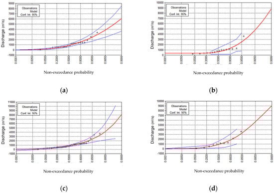
Figure 3. Estimation of floods based on maximum instantaneous discharge, (a) fitting of maximum instantaneous discharge at Meshrageh Station during 1966–2004; (b) fitting of maximum instantaneous discharge at Meshrageh Station during 2004–2019; (c) fitting of maximum instantaneous discharge at Meshrageh Station during 1966–2019; (d) maximum instantaneous discharge of the Ramshir Diversion Dam fitted using the Log-Pearson Type III distribution.

2.6. Flood Estimation Based on the Average Discharge

The flood estimation was completed based on the average discharge at Meshrageh station and Ramshir Diversion Dam. Next, the best distribution was selected based on the data available in different statistical periods. For Meshrageh station, the best distribution was normal distribution, and for Ramshir diversion dam, the best distribution was based on the lowest deviation from the log-normal distribution criterion. Figure 4 shows the fitting of the annual average of the Meshrageh and Ramshir diversion dam stations.

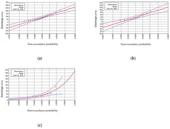
Figure 4. The fitting of the annual average of (a) Meshrageh stations 1966–2004, (b) Meshrageh stations 2004–2019; (c) Ramshir diversion dam stations.

2.7. Peak Flood Discharge with Different Return Periods and Flood Hydrograph

Many analytical methods were used to estimate flood peak flow [37,38]. These include extracting instantaneous discharge statistics, checking data conditions and statistical tests, fitting observational data with statistical distributions, testing the goodness of fit, and choosing a statistical distribution consistent with observational data, calculating the instantaneous peak discharge of floods with different return periods, and explaining flood hydrographs with varying periods of return. The data used was controlled and analyzed to perform statistical analyses, and then the statistical tests of independence, homogeneity, and outliers were used to control the observational data [39,40]. The independence test was performed to check the independence of the observational data and the non-effect of the data on each other. For this purpose, the Hyfran Plus software was used [36]. Consequently, according to the results of these evaluations, the data had the necessary conditions for the independence test and met the criteria for the independence test at the 5% significance level.

Homogeneity and outlier data tests were also performed on the available data. The homogeneity test was used to verify whether the data series were drawn from the same population. Each station’s observational data was divided into two parts for this test, and the statistical years were determined. The results of the investigation by Hyfran Plus software showed that all stations satisfied the homogeneity condition [36]. On the other hand, considering that outliers significantly affect statistical analysis, specifying and removing them was recommended. According to the United States Water Resources Council [41] recommendation, if the skewness coefficient is around ±4, there is no need to remove that data [41]. For this purpose, the outlier data test was applied to the long-term series of maximum instantaneous discharges, and the results showed that there is no outlier data for the upper and lower limit in the flood data of the stations, and there is no need to eliminate the flood data. Also, different hydrographs were extracted, including the hydrograph of the incoming flood to the Ramshir diversion dam, using the return period of the incoming discharges to the diversion dam station, the results of which are presented in Figure 5.

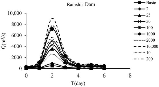
Figure 5. Flood hydrograph with different return periods of Ramshir diversion dam.

2.8. Electrical Conductivity (EC) Sampling Operation

Sampling operations to measure EC were carried out using the manual sampling method at depths of 0.2, 0.6, and 0.8 m from the bottom [42]. Therefore, a manual sampler was used to take samples at five stations along the river and at one additional station to assess the salinity of the Motbeg drainage. Sampling was conducted on a monthly basis, considering the river flow conditions during the sampling. Special attention was given when there was a possibility of changes in discharge or when the river diversion was in critical condition. The standard sampling procedure was applied, and the sampler was quickly plunged into the desired depth, kept at that depth for a while, and then pulled up [42].

EC was measured using a HACH Sension 378 conductivity meter (USA), which can measure EC in the range of approximately 0.001 µS/cm to 1000 mS/cm, with an accuracy of ≤0.5% of the measurement range. The instrument automatically compensates for temperature, with all readings adjusted to a reference temperature of 25 °C, ensuring consistency across measurements.

At each sampling location, three independent subsamples were collected and analyzed, and the mean value of the triplicate measurements was considered. The variability among replicates was generally low, with standard deviations not exceeding 3%, indicating high reproducibility and methodological robustness.

Given the low salinity of the study waters, it is acknowledged that the relationship between EC and salinity can be non-linear, and EC may not serve as a precise predictor of salinity or total dissolved solids (TDSs). Therefore, EC was used solely as a practical and internally consistent indicator of ionic concentration and water quality dynamics within the context of this site-specific case study. Figure 6 shows the HACH Sension 378 conductivity meter used in this study.

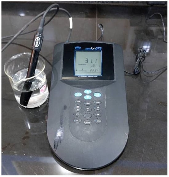
Figure 6. The HACH Sension 378 conductivity meter (USA) used in this study.

A linear correlation analysis was conducted to validate the EC measurements using independently obtained total dissolved solids (TDS) data. For this purpose, twelve representative water samples collected from the Meshrage station were analyzed. The TDS concentrations were determined gravimetrically, while EC was measured using a temperature-compensated conductivity probe. The results demonstrated a strong linear relationship between EC and TDS, yielding a correlation coefficient (R) of 0.975. This high correlation confirms the consistency and reliability of the EC data as a proxy for dissolved ionic content within the studied aqueous matrix.

The analysis of TDS and EC (Figure 7) data indicates that the relationship between these two variables is remarkably linear and consistent, such that the trend line TDS = 0.643·EC + 36.01 explains more than 97% of the variations in TDS. Examination of each point’s deviation from the central line shows that the maximum positive deviation is approximately 5.57%, while the maximum negative deviation is around 4.17%, with most points falling within ±3% of the trend line prediction.

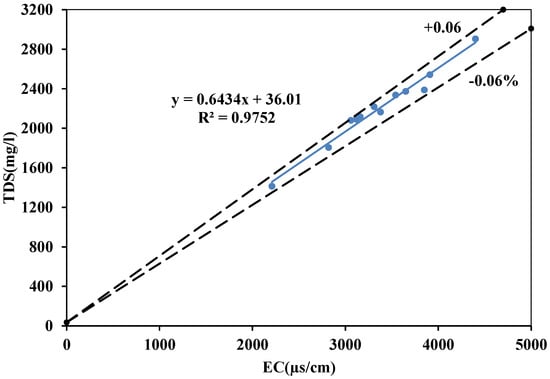
Figure 7. Correlation between EC and total dissolved solids (TDSs) in water samples from the Meshrage station.

Although a strong correlation is observed between EC and total dissolved solids (TDS), the relationship does not fully comply with the PSS-78 standard due to the low salinity of the water (<5 PSU). Consequently, EC has been employed as a relative and consistent indicator of salinity dynamics to monitor both temporal and spatial variations in water quality. This approach enables the assessment of relative salinity trends in low-salinity environments, where conventional TDS-based methods may be subject to higher uncertainty.

2.9. Numerical Modeling

The MIKE 11 model was used to simulate river flow and salinity in this project. This model can simulate various structures, such as bridges and spur dike. With advanced graphical capabilities, the model is able to analyze flow conditions in an unsteady state with high accuracy [42,43,44]. This model can simulate and solve the steady and unsteady flow equations and hydrodynamics of the channel network and simulate sediment transport and river quality [45,46]. Preparing the required data to establish the river model involves four items: the route network, cross-sections, boundary conditions, and hydraulic parameters [47]. For the route network, the model must be given a network to check the path. Considering the long length of the route and the presence of many twists and turns from the lower part of the Ramshir diversion Dam to the Shadegan Wetland, Google Earth extracted the desired route, and then the flow path was determined by GIS software [48,49]. Figure 8 shows the path network created in the MIKE 11 software.

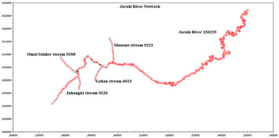
Figure 8. The plan of the Jarahi River and the network of streams in the MIKE 11 model with the names of the river branches.

MIKE 11 is a versatile and modular engineering tool for modeling 1D hydrodynamic conditions in rivers, lakes/reservoirs, irrigation canals, and other inland water systems. It is a fully dynamic modeling tool for the detailed analysis, design, management, and operation of both simple and complex river and channel systems. The hydrodynamic (HD) model is the nucleus of the MIKE 11 modeling system and forms the basis for the simulation of flood inundation. The HD model can simulate 1D unsteady flow in a network of rivers. The result of the HD simulation consists of a time series of water levels and discharges at various points along the river system. MIKE 11 HD provides a choice among three different flow descriptions, namely kinematics, diffusive, and dynamic wave approaches. MIKE 11 HD solves the Saint-Venant equations to obtain the hydrodynamic state of the river networks. The post-processor tool of MIKE 11 is the MIKEVIEW, which helps to view and analyze the results through graphical and animated interfaces. The governing equations in MIKE 11 are 1D shallow water type, which are the modifications of the basic Saint-Venant equations. The Saint-Venant equations representing conservation of mass and momentum are Equations (1) and (2), respectively, as given below.

$${\displaystyle \frac{\partial Q}{\partial X}}+{\displaystyle \frac{\partial A}{\partial t}}=q$$

(1)

$${\displaystyle \frac{\partial Q}{\partial t}}+{\displaystyle \frac{\partial \left[\gamma \frac{Q^2}{A}\right]}{\partial X}}+gA{\displaystyle \frac{\partial H_1}{\partial X}}+{\displaystyle \frac{gQ\left|Q\right|}{C^{2}AR}}=0$$

(2)

where Q = discharge (m³/s); A = flow area (m²); q = lateral inflow (m²/s); H₁ = stage above datum; c = Chezy’s resistance coefficient (m^1/2/s); R = hydraulic radius (m); ᵞ = momentum distribution coefficient; g = acceleration due to gravity (9.81 m²/s); X = longitudinal distance in the direction of flow (m); and t = elapsed time(s). Equations (1) and (2) are transformed to a set of implicit finite difference equations and solved using double sweeping algorithm [50]. The computational grid comprises alternating Q and H₁ points automatically generated by the model, based on user requirements. Q points are always placed midway between neighboring H₁ points. H₁ points are located at cross-sections or at equidistant intervals in between if the distance between cross-sections is greater than the maximum space interval, dx, specified by the users.

The one-dimensional advection-dispersion (AD) equation is expressed as follows:

$${\displaystyle \frac{\partial c}{\partial t}}+u{\displaystyle \frac{\partial c}{\partial x}}=D{\displaystyle \frac{{\partial }^{2}c}{\partial x^2}}+S_c+K_c$$

(3)

In this equation, u, D, C, S_c, and K_c represent the flow velocity, longitudinal dispersion coefficient, concentration, source or sink term of pollution, and the rate of production or decay within the element, respectively. The MIKE 11 software considers production or decay as a first-order process; therefore, the production or decay term is expressed as K_c in first order.

Regarding the cross-sections, the specifications of the cross-sections of the Jarahi River and the traditional channels in 2013 were prepared by the KWPA. In this research, due to the lack of adequate cross-sectional information, mapping was performed in places that had not been mapped before. However, the total number of cross-sections used in this project was 200 cross-sections, of which 165 cross-sections were related to the stretch of the Jarahi River from the Ramshir diversion Dam to the Shadegan Wetland station, and 35 cross-sections were related to traditional channels. It is worth mentioning that, in addition to the geometric characteristics of the desired sections, information about the mileage of each section from the beginning of the interval should be entered into the model. In this project, according to each cross-section’s $x$ and $y$ coordinates, the sections’ distances were calculated and entered the data model using global coordinates [48,49].

Figure 9 in the following presents several examples of river cross-sections at different river kilometer locations in the MIKE 11 model.

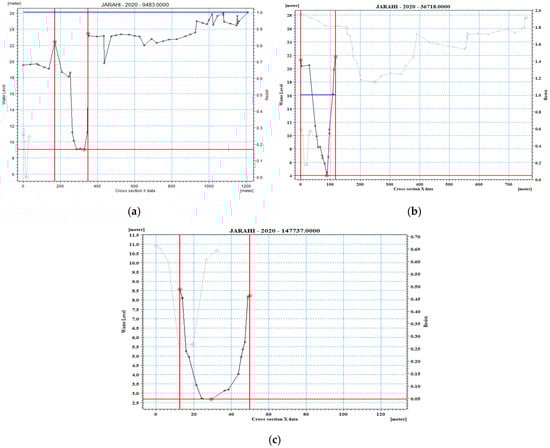
Figure 9. Several examples of Jarahi River cross-sections in the MIKE 11 Model. (a) Cross-section of the Jarahi River at 9.48 km; (b) cross-section of the Jarahi River at 36.71 km; (c) cross-section of the Jarahi River at 147.73 km.

Regarding the boundary conditions, it is necessary to enter the boundary conditions with the daily discharge in the main river and the water level in the downstream part at the endpoint of the model. In this study, the hydrometric station of the Ramshir diversion Dam upstream was considered the upstream boundary condition, and the Gauge-time data in the Shadegan station, corresponding to a specific time series with the upstream boundary conditions, was considered the downstream boundary condition. At the end of each sub-bank path, the model entered the boundary condition in the form of normal calculation depth. At the last step, the necessary flow parameters, including roughness coefficient, initial conditions, wave types, etc., were used as hydrodynamic parameters in the edit file for this simulation model. In this project, the Soil Conservation Service (SCS) method was used to determine Manning’s roughness coefficient according to the type of River and traditional channels [51]. The value of base n was considered equal to 0.02 due to the sandy nature of the riverbed. On the other hand, considering the effect of vegetation, the modification factor for vegetation cover was 0.01, and the effect factor of vegetation volume was omitted because there was no dense vegetation or weed growth in the river path. For this reason, the roughness coefficient for modeling in this river was considered equal to 0.03.

3. Results

3.1. Calibration of the MIKE 11 Model

This research determined the roughness coefficient based on the method used to control the water level and discharge in the river, which is essential to solving the flow problem. The Manning’s n was set up at 0.03 for the whole area. The MIKE 11 model was adjusted and modeled according to the qualitative and quantitative statistics of the Jarahi River in the water year of 2019, July to September, and according to the latest cross-sections of the Jarahi River. At upstream, the outflows hydrograph from Ramshir Dam were considered and at downstream, Shadegan’s discharge-gauge hydrograph curve was chosen as the final point of the model. Figure 10 shows the input and output boundary conditions of the calibration model.

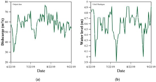
Figure 10. (a) Input boundary condition to the model (output discharge from Ramshir dam from 1 July to 31 September 2019); (b) output boundary condition to the model (Gauge Shadegan, period 1 July to 31 September 2019).

In addition, according to the traditional streams selected for this project, the inlet flows to each stream in the summer period of 2019 were added to the model. In traditional dams, according to the geographical location of the streams, the amount of flow entering the Jahangiri stream was 50% higher than the other streams, which was due to the proximity of the stream to the Shahid Hemat Dam. Further, due to the location of the Omal Sakher stream, the ground level in this stream was higher than the bottom of the Jarahi River, and the inlet discharge to this stream was zero.

Figure 11 depicts the validation of the numerical model results with the data. The model’s accuracy was verified by comparing the numerical results with the observed data for the water surface profile hydrograph and the flow discharge hydrograph at the Gorgor station cross-section. The comparison of discharge and water surface profile at the Gorgor station, which was used as the validation point for the numerical model, indicated an error of less than 10%.

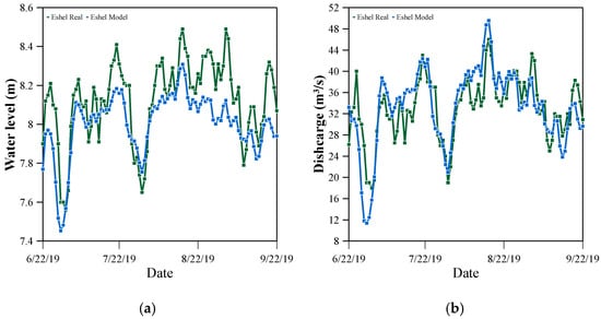
Figure 11. (a) Water level profile control at Gorgor station; (b) discharge control at Gorgor station.

Field measurements were carried out, in different parts of the river, to investigate drainage’s effect on the salinity of the river flow. According to Table 7, salinity changes occurred in different months of the year, and October had the highest salinity among the months of the year. The reasons were the discharge reduction of the river at the end of the water year and increasing the pollutants in the river due to the flow of drains.

Table 7. EC values of the Jarahi River measured at different locations.

					EC (μS/cm)
Sections	Oct	Nov	Dec	Jan	Feb	Mar	Apr	May	Jun	Jul	Aug	Sep
Meshrageh	3580	2350	2990	3380	2690	3860	2970	3140	2230	*	*	*
After the intersection between the river and the drainage	6850	2740	9830	10,320	7560	*	3550	6150	2310	*	2470	*
Jarahi River, Gorgor	11,000	2560	4310		*	*	3390	5810	2039	*	7830	*
Jarahi River, Shahid Hemat	11,860	2720	7930		*	*	3230	6170	2530	*	*	*
Jarahi River, Shadegan	10,190	3500	6140		*	*	3220	5940	2540	*	19,280	*

*: No data available.

Several key issues were considered regarding the calibration of the model and the clarity of the salinity parameter in the hydrometric stations of the main River. These included considering the salinity for Motbeg drainage as a point source and the salinity in decentralized drains between Gorgor and Hemat Dam station as a distributed source. Such a process was also used in previous research study by Rice et al. [52]. In Figure 12, field-measured data are shown with a blue line, and numerical model results are shown with a red line at Gorgor station. Figure 12 indicates a good correlation between the field data and the numerical model.

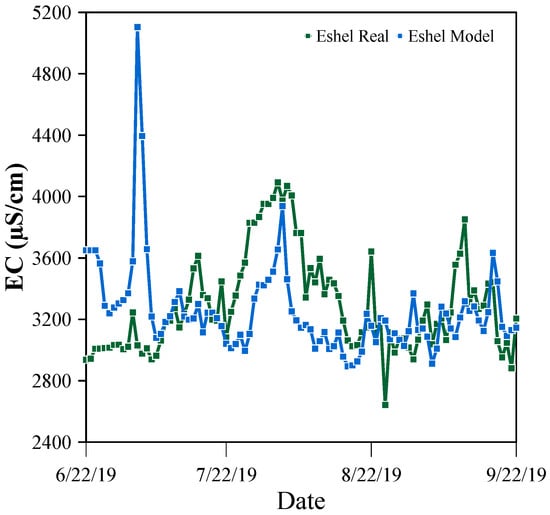
Figure 12. Water salinity control at Gorgor station.

The flow and salinity of the input to traditional channels were also calculated in the MIKE 11 model. According to the results obtained from the hydrodynamic analysis of the model, the Jahangiri channel yielded the highest output flow. The results showed that the salinity of the Mansuri and Gahan channels was almost the same due to their proximity. Based on the investigations, it was found that the most significant difference in their salinity was less than one percent. The same results were seen for Omal Sakher and Jahangiri channels. Finally, based on the calibration of the model at the Gorgor hydrometric stations, a good correlation (R² = 0.76) was observed between the field measurements and the numerical model predictions, indicating that the model successfully reproduces the dominant salinity patterns in the study area.

3.2. River Salinity in Low Discharges in Four Seasons

The minimum monthly discharges during the statistical period of the Meshrageh station were calculated and introduced as upstream boundary conditions to the model to determine the most critical qualitative mode of the Jarahi River in different seasons. Then, salinity distribution behavior was investigated along the Jarahi River and in its traditional channels during four scenarios in four seasons.

3.2.1. Autumn Season

This scenario investigated the salinity of the river in the autumn season. To this end, all required data, including the upstream and downstream boundary conditions under the average minimum discharges in different months of autumn for Meshrageh station and the minimum average gauge for Shadegan station, were introduced to MIKE 11. The average salinity for the upstream border conditions in October, November, and December was 3580, 2350, and 2990 µS/cm, respectively, according to the measured ECs. Figure 13 shows the changes in salinity over time in the section of Gorgor. According to the salinity diagram, the lowest and highest salinity levels in this station were in November at the rate of 3653 µS/cm and in December at the level of 5817 µS/cm. Also, in October, the average salinity was 4510 µS/cm. In this scenario, the highest salinity was observed when the discharge was minimal.

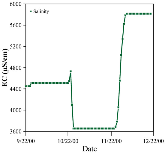
Figure 13. Changes in salinity to time in the Gorgor section in the first scenario.

The salinity in the traditional channels was also investigated, during which the lowest salinity occurred in November, while the highest occurred in December. Although the difference in salinity between the channels was slight, the highest salinity was at the branch of Omal Sakher, which was 6963 µS/cm in December. Figure 14 shows the estimated salinity level in traditional channels.

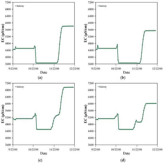
Figure 14. The salinity of the inlet water to the (a) Mansuri stream; (b) Gahan stream; (c) Omal Sakher stream; (d) Jahangiri stream.

3.2.2. Winter Season

The minimum discharge in this season was investigated considering the minimum discharge at Meshrageh station and the average minimum discharge at Shadegan station. According to the EC value measured in this research, the average salinity for upstream boundary conditions in January, February, and March was added to the model as 3380, 2690, and 3860 µS/cm, respectively. Figure 15 highlights the salinity changes over time in the Gorgor section in the second scenario. In this season, the lowest level of salinity was in January at 5981 µS/cm, and the highest level of salinity was in March at 8877 µS/cm. In February, the average salinity was 6140 µS/cm, showing the highest salinity at the lowest discharge.

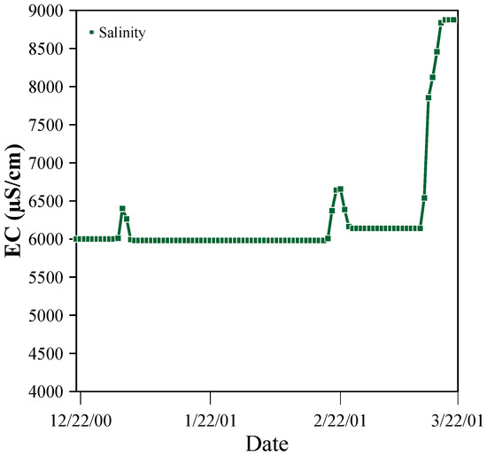
Figure 15. Changes in salinity with respect to time in the Gorgor section in the winter season.

The changes in salinity in the branched traditional streams under the second scenario show that in all streams, the lowest salinity occurred in January, while the highest salinity occurred in March. Further, like the first scenario, the Omal Sakher stream had the highest salinity of 10,340 µS/cm among all the streams. Figure 16 demonstrates the amount of salinity changes in traditional streams.

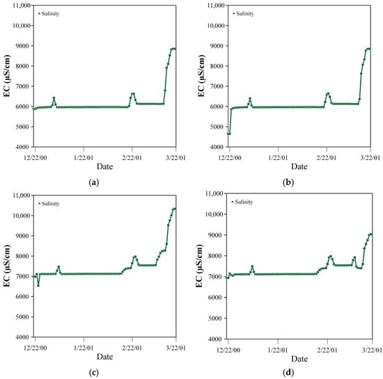
Figure 16. Input salinity to the (a) Gahan stream, (b) Mansuri stream, (c) Jahangiri stream, and (d) Omal Sakher stream, relative to the time in the fourth scenario in the second scenario.

3.2.3. Spring Season

In this section, the amount of salinity is analyzed according to the minimum discharge in the spring season. In this regard, the input data for the model, including the upstream and the downstream boundary conditions, were, respectively, the average minimum discharges during the statistical period of the Meshrageh station and the minimum gauge average at the Shadegan station. Figure 17 highlights the boundary conditions defined in Spring.

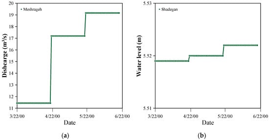
Figure 17. (a) The upstream boundary condition of the average minimum discharges in different months of spring at Meshrageh station; (b) the downstream boundary condition of the average minimum Gauges in different months of spring at Shadegan station.

For the qualitative boundary conditions of ECs, according to Table 7, the average salinity for the upstream boundary condition in April, May, and June was 2970, 3140, and 2230 µS/cm, respectively. According to the model results, the highest salinity in April was 8605 µS/cm. The lowest salinity was 5337 in June µS/cm. Furthermore, in this scenario, the average salinity in May at Gorgor station was 6470 µS/cm. The third scenario also showed the highest salinity at the lowest discharge in the Gorgor station (Figure 18).

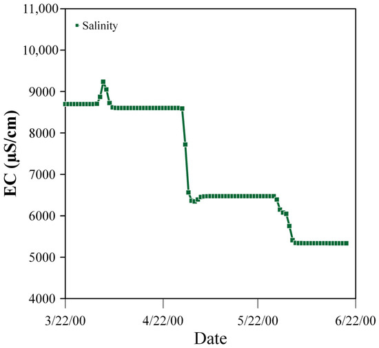
Figure 18. Changes in salinity with respect to time in the spring section of Gorgor.

Figure 19 depicts the changes in salinity with respect to time in the branched traditional streams. In these graphs, all streams have the lowest salinity in June and the highest salinity in April. Further, the Omal Sakher stream has the highest salinity by less than one percent compared to other streams.

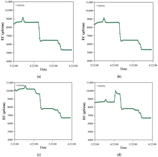
Figure 19. Input salinity to the (a) Gahan stream, (b) Mansuri stream, (c) Jahangiri stream, and (d) Omal Sakher stream, relative to the times in the fourth scenario and in the third scenario.

3.2.4. Summer Season

In the final scenario, the model was supplied with input and output data corresponding to the minimum discharge and the average of the lowest water level during the summer season. To this end, Meshrageh station was considered as the upstream boundary condition, and Shadegan station was considered as the downstream boundary condition. As stated in Table 7, the amount of EC for the scenario in the summer season was determined, which was considered the average salinity for the upstream boundary conditions. The salinity for the three months of summer in 2007, 1999, and 1877 µS/cm, respectively, showed the difference in salinity, which was less than one percent in the first two months of summer, which included July and August.

Figure 20 demonstrates the amount of salinity changes over time in the summer season. In this scenario, the difference in salinity between the highest month (July) and the lowest salinity in September was 1552 µS/cm. The salinity was 2993 µS/cm in September and 4545 µS/cm in July. Further, the average salinity in August was reported as 3580 µS/cm.

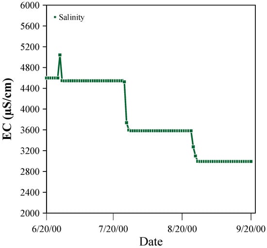
Figure 20. Changes in salinity to time in the Gorgor section in the fourth scenario.

In this scenario, the level of salinity was modeled for traditional streams. In all the streams, the lowest salinity and the highest salinity could be observed in September and July, respectively. Further, in the branch of Omal Sakher, the highest salinity occurred at the rate of 5790 µS/cm. Figure 21 highlights the level of salinity in the traditional network of streams.

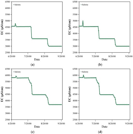
Figure 21. Input salinity to the (a) Gahan stream, (b) Mansuri stream, (c) Jahangiri stream, and (d) Omal Sakher stream, relative to the time in the fourth scenario.

For enhanced clarity and improved visual interpretation, the seasonal variations in salinity across the studied stations are illustrated in the form of a graphical representation (Figure 22). This visualization facilitates a more comprehensive understanding of temporal patterns and allows for clearer comparison of salinity fluctuations among different stations throughout the year.

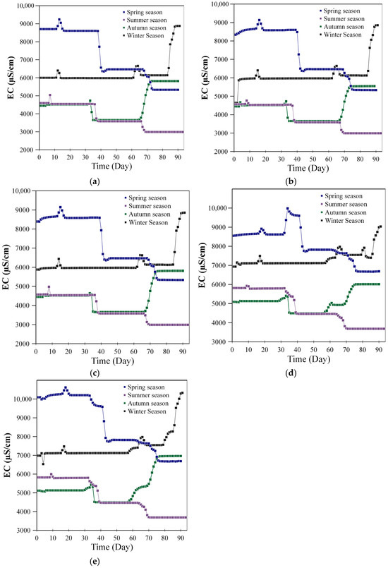
Figure 22. Input salinity to the (a) Gorgor section (b) Gahan stream, (c) Mansuri stream, (d) Jahangiri stream, and (e) Omal Sakher stream in all scenarios.

According to the presented scenarios, in the cold seasons of the year, the highest amount of salinity can be observed in the last month of the season, and in the warm seasons of the year, the highest amount of salinity can be observed in the first month of the season. Furthermore, among all the traditional streams, the highest amount of salinity in the whole year was reported for the Omal Sakher stream. In addition, according to different scenarios, some solutions are presented to reduce the salinity in the Jarahi River:

• Preventing Motbeg drainage from entering the Jarari River and transferring it to the Hadomeh stream.
• Preventing the entry of non-centralized drains between Gorgor station and Hemat dam and transferring it to Shadegan Wetland.
• Removing all the inlet drains (combining the previous two solutions).
• Increasing the output flow from Ramshir Dam (doubling the initial flow).

3.3. Investigation of Four Solutions to Reduce the Salinity in the Jarahi River

As seen in Figure 23a, the implementation of the first solution was effective. For average values, it was equal to 1266 µS/cm, which indicated a 39% decrease in salinity in the Gorgor station. In Figure 23a, the black and blue lines represent the EC before and after the implementation of the solution, respectively. Further, this solution caused a 32% decrease in salinity in the Mansuri stream and a 27% decrease in salinity in the Gahan stream.

Figure 23. (a) Comparison of salinity changes over time at Gorgor station, before and after the implementation of (a) the first salinity reduction strategy; (b) the second salinity reduction strategy; (c) the third strategy to reduce salinity; (d) the fourth strategy to reduce salinity.

The second solution was applied to reduce salinity in the region, considering the large number of non-centralized drains between Gorgor station and Hemat Dam and the relatively high water salinity of these drains. Figure 23b shows that this solution does not affect the reduction in salinity in the Gorgor section. Further, for the traditional streams in Mansuri and Gahan streams, their effect was zero percent, but for Jahangiri, up to a 21.4 percent reduction in salinity was observed.

The third work method, which was a combination of the two previous work methods, showed the effectiveness of the work method, which highlighted a 39% decrease in salinity in the Gorgor station in Figure 23c. It is also possible to point out a significant (40%) reduction in traditional streams in Mansuri and Gahan and 53% in the inlet of the Omal Sakher stream, which showed the applicability of this scenario in Figure 23c.

Finally, considering that the salinity of the river water at the site of the Ramshir diversion dam was relatively low, increasing the discharge from the dam can be considered a solution when it is not possible to divert or block the drains entering the river. According to this scenario, it can be seen in Figure 23d that the amount of salinity decreased by 23% in the Gorgor station. In the case of the traditional streams, a 22% decrease in the Mansuri and Gahan streams, as well as a 29% decrease in salinity at the Omal Sakher stream was detected.

Finally, it can be concluded that the third scenario, which includes the analysis of the salinity of the Jarahi River and the traditional Streams in the summer season under low discharge, has the highest decrease in salinity in the Jarahi River. On the other hand, Figure 24a–d show the salinity level according to the solutions mentioned for the Gahan, Jahangiri, Omal Sakher, and Mansuri streams. In Figure 24a, it can be seen a significant decrease in salinity and its approximate stability in the Gahan stream, according to the third solution, to the extent of 2000 µS/cm over time.

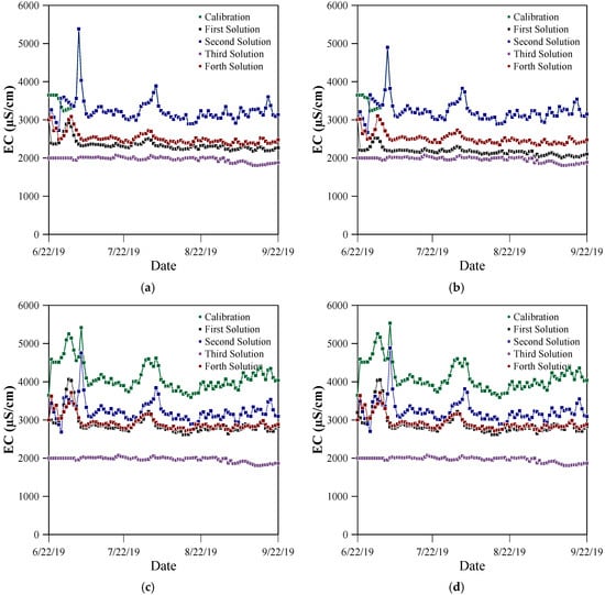
Figure 24. The amount of salinity in (a) the Gahan stream, (b) the Mansuri stream, (c) the Omal Sakher stream, and (d) the Jahangiri stream.

Figure 24b highlights the amount of salinity reduction in each solution. According to the solutions presented in this stream, the salinity level of garlic remains the same during different months. Although according to the second solution, the amount of salinity was not decreased significantly, and a comparison of the solutions showed that the salinity of the third solution decreased by 60%.

Although Figure 24c and Figure 21d show Omal Sakher and Jahangiri streams, other solutions keep the salinity in a constant range of approximately 5000 µS/cm to 3000 µS/cm. The third solution, like other streams, reduces salinity by 60% and keeps it in a constant range of 2000 µS/cm, which has a significant impact on agriculture and industry in our study area.

4. Discussion

In the current research, the effectiveness of different parameters and their role in reducing salinity in rivers and traditional canals can be recognized. Considering that Kumar et al. [53] evaluated the MIKE11 model and confirmed its effectiveness for water resource management during dry years, the MIKE 11 modeling conducted in this project for the Jarahi River can also make a significant contribution to reducing salinity in traditional canals an essential issue in agriculture, which remains an important challenge for agricultural sustainability in the region. Kale et al. [47] also examined the effectiveness of MIKE 11 modeling in unsteady flows; however, they did not propose specific solutions for salinity control. In contrast, this project, using the available data, not only demonstrates the effectiveness of the modeling approach but also provides scenario-based and practically applicable strategies to reduce salinity in a long river stretch and to study and mitigate salinity in traditional canals along the river. These strategies could be highly beneficial for farmers and for water resource management both in the study area and in other regions in the future. Furthermore, Adib and Javdan [21] investigated salinity in the tidal Karun River using numerical and statistical models to assess salinity levels.

The consistency between field observations, seasonal discharge conditions, and the simulated salinity response highlights a strong internal coherence of the results obtained in this study. In particular, the higher effectiveness of flow regulation and drainage control scenarios under low-flow conditions agrees with the behavior reported by Kumar et al. and Adib and Javdan in similar regulated river systems, which supports the external consistency of the findings. At the same time, the scenario-based focus of the present study extends previous MIKE 11 applications, such as those discussed by Kale et al. [47] by linking hydrodynamic modeling outcomes to explicit salinity reduction strategies rather than purely hydraulic analyses. However, in this study, various scenarios under minimum discharge conditions and across different seasons of the year were used to comprehensively analyze salinity and evaluate the effectiveness of the proposed solutions for reducing salinity in the Jarahi River area. The results suggest that the proposed management scenarios can contribute to salinity control and improved agricultural productivity in the region, as well as in other case studies facing similar or related salinity challenges.

5. Conclusions

Jarahi River, which is one of the most important rivers in Iran for human industry and agriculture, is facing the challenge of water salinity. Therefore, in present research, numerical and field studies were conducted to improve the quantitative and qualitative problems of water resources management downstream of Ramshir Diversion Dam to Shadegan Wetland. This research was conducted using field data collection and numerical simulation using the MIKE 11 model. According to the minimum discharge scenarios in different months of the year, the salinity level along the Jarahi River was observed. The highest salinity level was reported in the months of March and April in the Jarahi River and traditional streams. On the other hand, the amount of EC was investigated in different areas and different months of the year along the Jarahi River. The results showed that the highest salinity changes occurred in October. Four scenarios were proposed to reduce salinity in the Jarahi River.

• The highest salinity reduction observed at the Gorgor section was under the first and third scenarios, with a 39% decrease (about 1266 µS/cm).
• In the second scenario, the salinity in the Gorgor section did not change, while in the other streams, such as the Mansuri and Gahan streams, the salinity fell to zero.
• In the traditional streams, the most significant reduction was seen within the Mansuri stream and at the mouth of the Omal Sakher stream, where salinity would decrease by 53% due to the third scenario.
• Increasing the release flow from the Ramshir Dam was also effective, yielding a reduction of 724 µS/cm, or about 23%, at the Gorgor station.
• In the case of the salinity trend at the entrance of the traditional Jahangiri stream, there was a consistent decrease in all proposed scenarios.
• The results indicated that scenario-based management was important for salinity reduction and efficiency improvement in the utilization of water resources.
• The study also showed that the MIKE 11 model was a useful tool for simulating salinity dynamics under given regional conditions and applied management scenarios.

Through this study, both qualitative and quantitative analyses of salinity were conducted, representing a novel contribution to the field of salinity control in river systems. The findings demonstrated that the proposed approach significantly reduces water salinity in the Jarahi River, which is essential for the preservation of local water resources. In addition to developing and testing control strategies for the study area, the results confirmed the applicability of hydrodynamic modeling for managing salinity in long river reaches and for evaluating the impacts of diversion dams. These outcomes provide valuable insights for predicting salinity trends, supporting decision-making, and improving the management of water resources for both agricultural and human use.

References

- Mishra, R.K. Fresh water availability and its global challenge. Br. J. Multidiscip. Adv. Stud. 2023, 4, 1–78. [Google Scholar] [CrossRef]
- Bazzi, H.; Ebrahimi, H.; Aminnejad, B. A comprehensive statistical analysis of evaporation rates under climate change in Southern Iran using WEAP (Case study: Chahnimeh Reservoirs of Sistan Plain). Ain Shams Eng. J. 2021, 12, 1339–1352. [Google Scholar] [CrossRef]
- Khazaei Moughani, S.; Rezazadeh, S.; Azimmohseni, M.; Rahi, G.; Bahmanpouri, F. Applying a transfer function model to improve the sediment rating curve. Int. J. River Basin Manag. 2025, 23, 313–325. [Google Scholar] [CrossRef]
- Rezazadeh, S.; Manafpour, M.; Bahmanpouri, F.; Gualtieri, C. Application of the entropy model to estimate flow discharge and bed load transport in a large river. Phys. Fluids 2025, 37, 023325. [Google Scholar] [CrossRef]
- Melad, R.S.; Nonato, R.L.V.; Salazar, D.J.; Ligaray, M.V.; Choi, A.E.S. Spatial assessment of water quality in Mananga River in Talisay City, Cebu, Philippines. Results Eng. 2024, 24, 103030. [Google Scholar] [CrossRef]
- Sajjadi, S.M.; Barihi, S.; Ahadiyan, J.; Azizi Nadian, H.; Valipour, M.; Bahmanpouri, F.; Khedri, P. Redesigning the fuse plug, emergency spillway, and flood warning system: An application of flood management. Water 2024, 16, 3694. [Google Scholar] [CrossRef]
- Nadian, H.A.; Karamzadeh, N.S.; Ahadiyan, J.; Bakhtiari, M. Trajectory and spreading of falling circular dense jets in shallow stagnant ambient water. Results Eng. 2024, 24, 102897. [Google Scholar] [CrossRef]
- Casila, J.C.C.; Nicolas, M.D.; Duka, M.; Haddout, S.; Priya, K.L.; Yokoyama, K. Assessing dissolved oxygen dynamics in Pasig River, Philippines: A HEC-RAS modeling approach during the COVID-19 pandemic. Water Pract. Technol. 2024, 19, 1365–1381. [Google Scholar] [CrossRef]
- Quinn, N.W. Adaptive implementation of information technology for real-time, basin-scale salinity management in the San Joaquin Basin, USA and Hunter River Basin, Australia. Agric. Water Manag. 2011, 98, 930–940. [Google Scholar] [CrossRef]
- Lewis, E.L.; Perkin, R.G. Salinity: Its definition and calculation. J. Geophys. Res. Oceans 1978, 83, 466–478. [Google Scholar] [CrossRef]
- Leite, T.; Branco, P.; Ferreira, M.T.; Santos, J.M. Activity, boldness and schooling in freshwater fish are affected by river salinization. Sci. Total Environ. 2022, 819, 153046. [Google Scholar] [CrossRef] [PubMed]
- Mohammadzadeh-Habili, J.; Khalili, D.; Zand-Parsa, S.; Sabouki, A.; Dindarlou, A.; Mozaffarizadeh, J. Influences of natural salinity sources and human actions on the Shapour River salinity during the recent streamflow reduction period. Environ. Monit. Assess. 2021, 193, 696. [Google Scholar] [CrossRef] [PubMed]
- Melesse, A.M.; Khosravi, K.; Tiefenbacher, J.P.; Heddam, S.; Kim, S.; Mosavi, A.; Pham, B.T. River water salinity prediction using hybrid machine learning models. Water 2020, 12, 2951. [Google Scholar] [CrossRef]
- Bhuiyan, M.J.A.N.; Dutta, D. Assessing impacts of sea level rise on river salinity in the Gorai river network, Bangladesh. Estuar. Coast. Shelf Sci. 2012, 96, 219–227. [Google Scholar] [CrossRef]
- Rice, K.C.; Hong, B.; Shen, J. Assessment of salinity intrusion in the James and Chickahominy Rivers as a result of simulated sea-level rise in Chesapeake Bay, East Coast, USA. J. Environ. Manag. 2012, 111, 61–69. [Google Scholar] [CrossRef]
- Xiao, H.; Huang, W.; Johnson, E.; Lou, S.; Wan, W. Effects of sea level rise on salinity intrusion in St. Marks River Estuary, Florida, USA. J. Coast. Res. 2014, 68, 89–96. [Google Scholar] [CrossRef]
- Uncles, R.J.; Stephens, J.A. The effects of wind, runoff and tides on salinity in a strongly tidal sub-estuary. Estuaries Coasts 2011, 34, 758–774. [Google Scholar] [CrossRef]
- Vale, L.M.; Dias, J.M. The effect of tidal regime and river flow on the hydrodynamics and salinity structure of the Lima Estuary: Use of a numerical model to assist on estuary classification. J. Coast. Res. 2011, 1604–1608. [Google Scholar]
- Koutsoyiannis, D. Revisiting global hydrological cycle: Is it intensifying? Hydrol. Earth Syst. Sci. Discuss. 2020, 1–49. [Google Scholar] [CrossRef]
- Qureshi, A.S.; Qadir, M.; Heydari, N.; Turral, H.; Javadi, A. A Review of Management Strategies for Salt-Prone Land and Water Resources in Iran; IWMI Working Paper 125; IWMI: Colombo, Sri Lanka, 2007; ISBN 978-92-9090-681-0. [Google Scholar]
- Adib, A.; Javdan, F. Interactive approach for determination of salinity concentration in tidal rivers (Case study: The Karun River in Iran). Ain Shams Eng. J. 2015, 6, 785–793. [Google Scholar] [CrossRef]
- Siles-Ajamil, R.; Díez-Minguito, M.; Losada, M.Á. Tide propagation and salinity distribution response to changes in water depth and channel network in the Guadalquivir River Estuary: An exploratory model approach. Ocean Coast. Manag. 2019, 174, 92–107. [Google Scholar] [CrossRef]
- Farahani, N.D.; Shahraiyni, H.T.; Sheikhi, R. Water quality modeling for determination of suitability of water for shrimp farming in tidal rivers. Water Qual. Res. J. 2019, 54, 34–46. [Google Scholar] [CrossRef]
- Matsoukis, C.; Amoudry, L.O.; Bricheno, L.; Leonardi, N. Numerical investigation of river discharge and tidal variation impact on salinity intrusion in a generic river delta through idealized modelling. Estuaries Coasts 2023, 46, 57–83. [Google Scholar] [CrossRef]
- Zhang, Z.; Cui, B.; Zhao, H.; Fan, X.; Zhang, H. Discharge–salinity relationships in Modaomen waterway, Pearl River estuary. Procedia Environ. Sci. 2010, 2, 1235–1245. [Google Scholar] [CrossRef]
- Jeong, S.; Yeon, K.; Hur, Y.; Oh, K. Salinity intrusion characteristics analysis using EFDC model in the downstream of Geum River. J. Environ. Sci. 2010, 22, 934–939. [Google Scholar] [CrossRef]
- AL-Thamiry, H.A.K.; Haider, F.A. Salinity variation of Euphrates River between Ashshinnafiyah and Assamawa Cities. J. Eng. 2013, 19, 1442–1466. [Google Scholar] [CrossRef]
- Dimitriadis, P.; Koutsoyiannis, D.; Iliopoulou, T.; Papanicolaou, P. A global-scale investigation of stochastic similarities in marginal distribution and dependence structure of key hydrological-cycle processes. Hydrology 2021, 8, 59. [Google Scholar] [CrossRef]
- Sadodin, A.; Rostam Assl, F.; Ownegh, M.; Armin, M.A. Assessing the vulnerability of the river systems in the Jarahi River Basin. J. Water Soil Conserv. 2020, 27, 47–68. [Google Scholar] [CrossRef]
- Raeisi, N.; Moradi, S.; Scholz, M. Surface water resources assessment and planning with the QUAL2Kw model: A case study of the Maroon and Jarahi Basin (Iran). Water 2022, 14, 705. [Google Scholar] [CrossRef]
- Chenrai, S.A.; Nadian, H.A.; Ahadiyan, J.; Valipour, M.; Oliveto, G.; Sajjadi, S.M. Enhancing hydraulic efficiency of side intakes using spur dikes: A case study of Hemmat Water Intake, Iran. Water 2024, 16, 2254. [Google Scholar] [CrossRef]
- Ahadiyan, J.; Chenari, S.A.; Nadian, H.A.; Katopodis, C.; Valipour, M.; Sajjadi, S.M.; Omidvarinia, M. Sustainable systems engineering by CFD modeling of lateral intake flow with flexible gate operations to improve efficient water supply. Int. J. Sediment Res. 2024, 39, 629–642. [Google Scholar] [CrossRef]
- Tian, X.; Zhang, X.; Wu, Y. Classification of planted forest species in southern China with airborne hyperspectral and LiDAR data. J. For. Res. 2020, 25, 369–378. [Google Scholar] [CrossRef]
- Buchroithner, M.F.; Pfahlbusch, R. Geodetic grids in authoritative maps—New findings about the origin of the UTM Grid. Cartogr. Geogr. Inf. Sci. 2017, 44, 186–200. [Google Scholar] [CrossRef]
- Wagner, C.R.; Mueller, D.S. Comparison of bottom-track to global positioning system referenced discharges measured using an acoustic Doppler current profiler. J. Hydrol. 2011, 401, 250–258. [Google Scholar] [CrossRef]
- Mohamadi, M.; Mamizadeh, J.; Ehsanzadeh, E. Comparison of statistical and empirical models in determining the intensity–duration–frequency rainfall curves (case study: Ilam city). Irrig. Water Eng. 2020, 11, 256–268. [Google Scholar] [CrossRef]
- Samantaray, S.; Sahoo, A. Estimation of flood frequency using statistical method: Mahanadi River basin, India. H2Open J. 2020, 3, 189–207. [Google Scholar] [CrossRef]
- Fitri, A.; Hadie, M.S.N.; Agustina, A.; Pratiwi, D.; Susarman, S.; Pramita, G.; Salah, H.A. Analyses of flood peak discharge in Cimadur river basin, Banten Province, Indonesia. E3S Web Conf. 2021, 331, 08006. [Google Scholar] [CrossRef]
- Crochemore, L.; Isberg, K.; Pimentel, R.; Pineda, L.; Hasan, A.; Arheimer, B. Lessons learnt from checking the quality of openly accessible river flow data worldwide. Hydrol. Sci. J. 2020, 65, 699–711. [Google Scholar] [CrossRef]
- de Gois, G.; de Oliveira-Júnior, J.F.; da Silva Junior, C.A.; Sobral, B.S.; de Bodas Terassi, P.M.; Junior, A.H.S.L. Statistical normality and homogeneity of a 71-year rainfall dataset for the state of Rio de Janeiro—Brazil. Theor. Appl. Climatol. 2020, 141, 1573–1591. [Google Scholar] [CrossRef]
- U.S. Water Resources Council, Hydrology Committee. Guidelines for Determining Flood Flow Frequency; U.S. Government Printing Office: Washington, DC, USA, 1975; Bulletin 17.
- Shi, B.; Catsamas, S.; Kolotelo, P.; Wang, M.; Lintern, A.; Jovanovic, D.; McCarthy, D.T. A low-cost water depth and electrical conductivity sensor for detecting inputs into urban stormwater networks. Sensors 2021, 21, 3056. [Google Scholar] [CrossRef]
- Pinos, J.; Timbe, L.; Timbe, E. Evaluation of 1D hydraulic models for the simulation of mountain fluvial floods: A case study of the Santa Bárbara River in Ecuador. Water Pract. Technol. 2019, 14, 341–354. [Google Scholar] [CrossRef]
- Liu, Y.; Wang, F.; Li, Y.; Cai, Z.; Xu, T.; Chen, Y. Source analysis of total nitrogen in a representative seaward river using the calibrated MIKE model. Water Qual. Res. J. 2025, wqrj2025102. [Google Scholar] [CrossRef]
- DHI. MIKE 11: A Modelling System for Rivers and Channels—Reference Manual; DHI–Water and Development: Hørsholm, Denmark, 2003. [Google Scholar]
- DHI. MIKE FLOOD: 1D–2D Modelling—User Manual; DHI: Hørsholm, Denmark, 2009. [Google Scholar]
- Kale, M.U.; Nagdeve, M.B.; Wadatkar, S.B.; Deshmukh, M.M.; Mankar, A.N. Hydraulic impact of Wan River project with MIKE 11. Agric. Eng. Int. CIGR J. 2014, 16, 21–31. [Google Scholar]
- Henshaw, A.J.; Sekarsari, P.W.; Zolezzi, G.; Gurnell, A.M. Google Earth as a data source for investigating river forms and processes: Discriminating river types using form-based process indicators. Earth Surf. Process. Landf. 2020, 45, 331–344. [Google Scholar] [CrossRef]
- Popescu, C.; Bărbulescu, A. Floods simulation on the Vedea River (Romania) using hydraulic modeling and GIS software: A case study. Water 2023, 15, 483. [Google Scholar] [CrossRef]
- Abbott, M.B.; Ionescu, F. On the numerical computation of nearly horizontal flows. J. Hydraul. Res. 1967, 5, 97–117. [Google Scholar] [CrossRef]
- Arcement, G.J.; Schneider, V.R. Guide for Selecting Manning’s Roughness Coefficients for Natural Channels and Flood Plains; U.S. Geological Survey: Washington, DC, USA, 1989; Water-Supply Paper 2339. [CrossRef]
- Fakouri, B.; Mazaheri, M.; Samani, J.M. Management scenarios methodology for salinity control in rivers (case study: Karoon River, Iran). J. Water Supply Res. Technol. AQUA 2019, 68, 74–86. [Google Scholar] [CrossRef]
- Kumar, K.S.; Galkate, R.V.; Tiwari, H.L. River basin modelling for Shipra River using MIKE BASIN. ISH J. Hydraul. Eng. 2021, 27, 188–199. [Google Scholar] [CrossRef]
Disclaimer/Publisher’s Note: The statements, opinions and data contained in all publications are solely those of the individual author(s) and contributor(s) and not of MDPI and/or the editor(s). MDPI and/or the editor(s) disclaim responsibility for any injury to people or property resulting from any ideas, methods, instructions or products referred to in the content. |
© 2026 by the authors. Licensee MDPI, Basel, Switzerland. This article is an open access article distributed under the terms and conditions of the Creative Commons Attribution (CC BY) license.