
Deep Learning-Based Daily Streamflow Prediction Model for the Hanjiang River Basin

Abstract
1. Introduction
2. Methodology
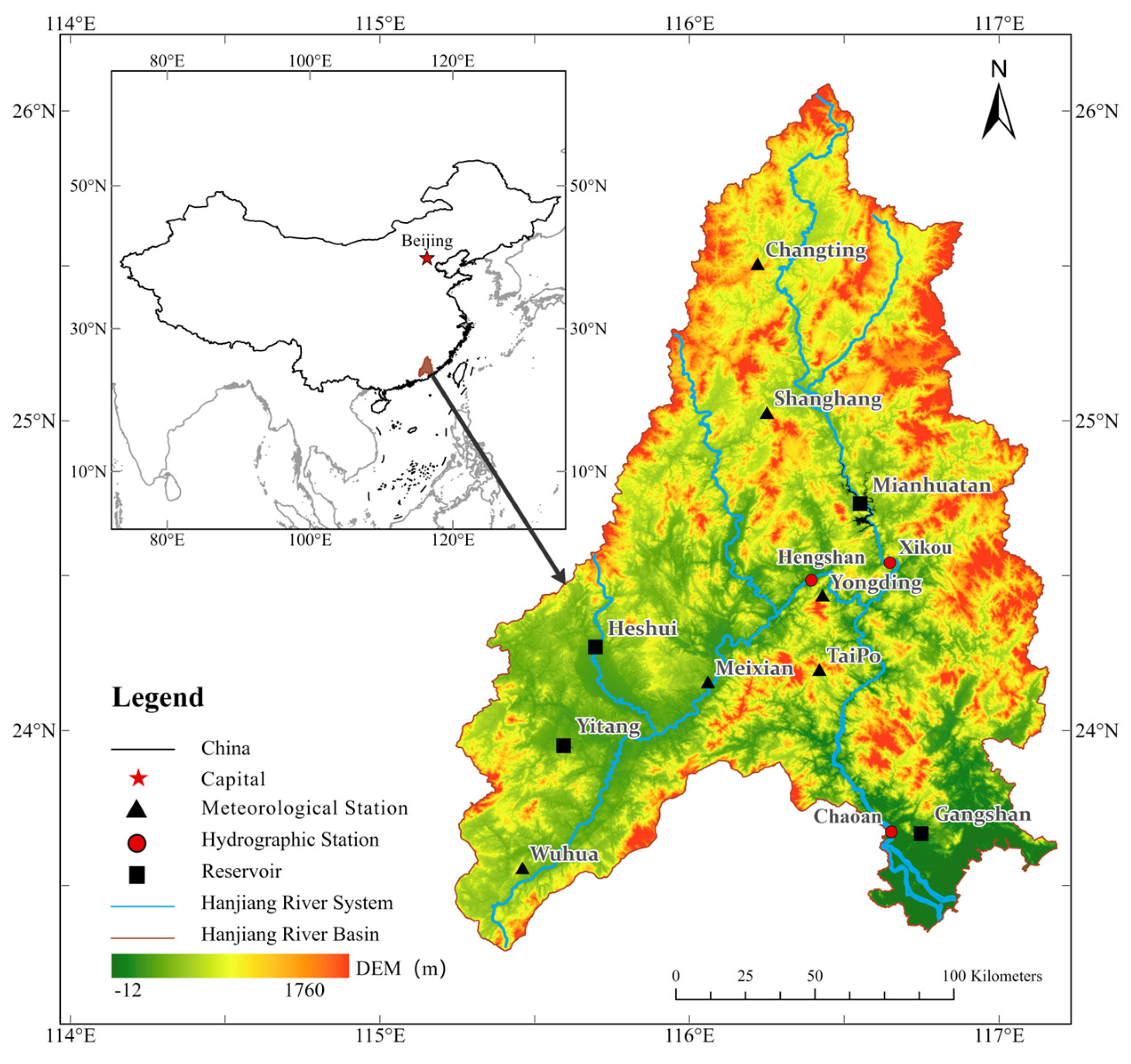
2.1. Study Area
2.2. Dataset
2.3. Deep Learning Models
2.3.1. MLP
2.3.2. CNN
2.3.3. GRU and BiLSTM
2.3.4. SA
2.3.5. Coupled Model
2.3.6. Training and Hyperparameter Optimization
2.4. Model Evaluation Method
2.5. Flood Event Recognition
2.6. Prediction Interval Estimation
2.7. Shapley Additive Explanations
3. Results and Discussion
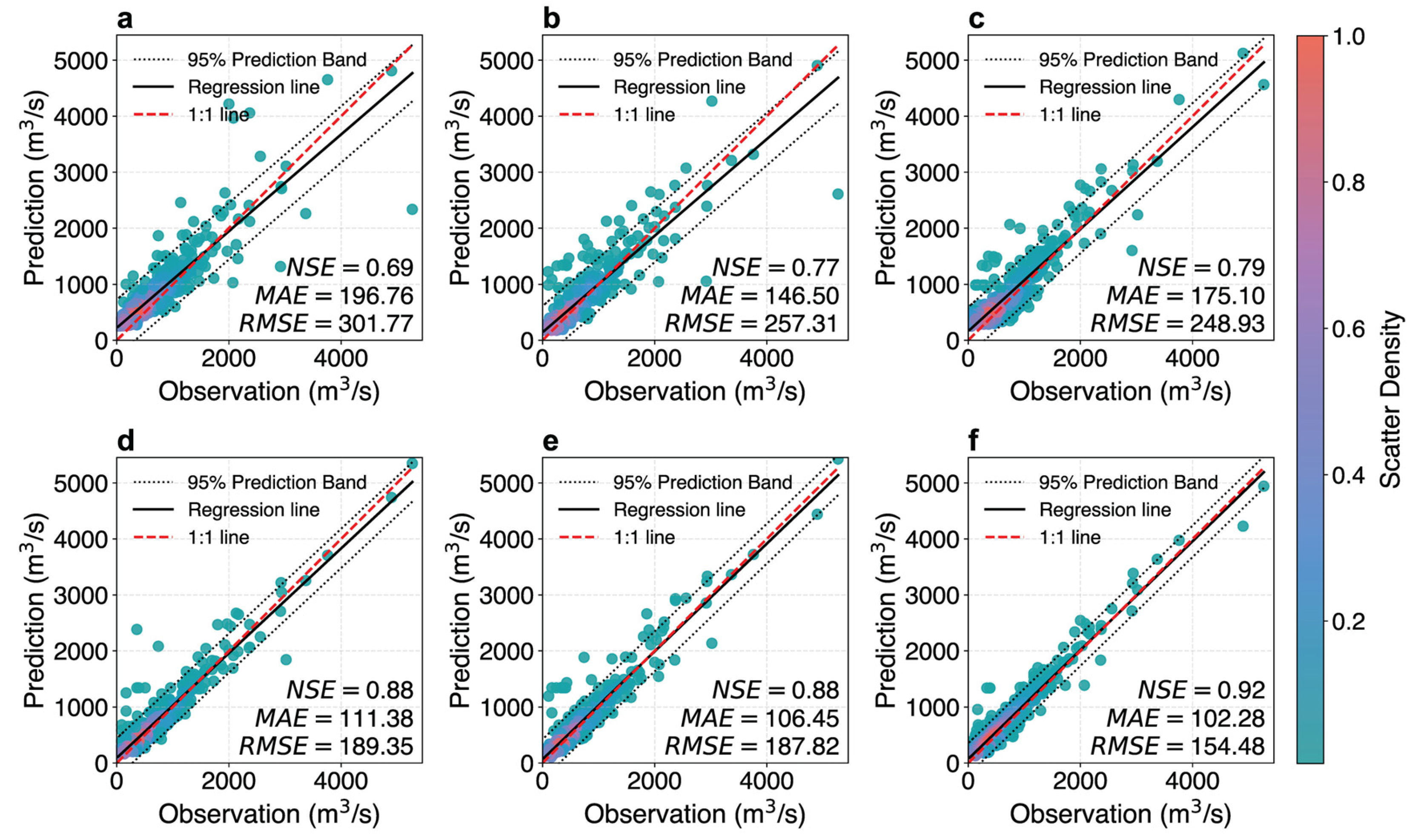
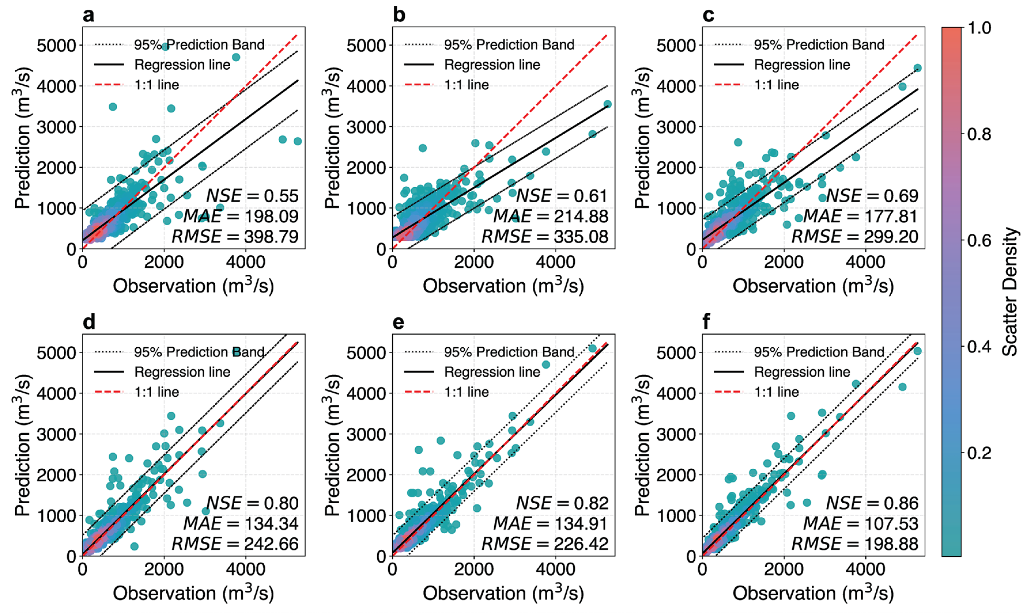
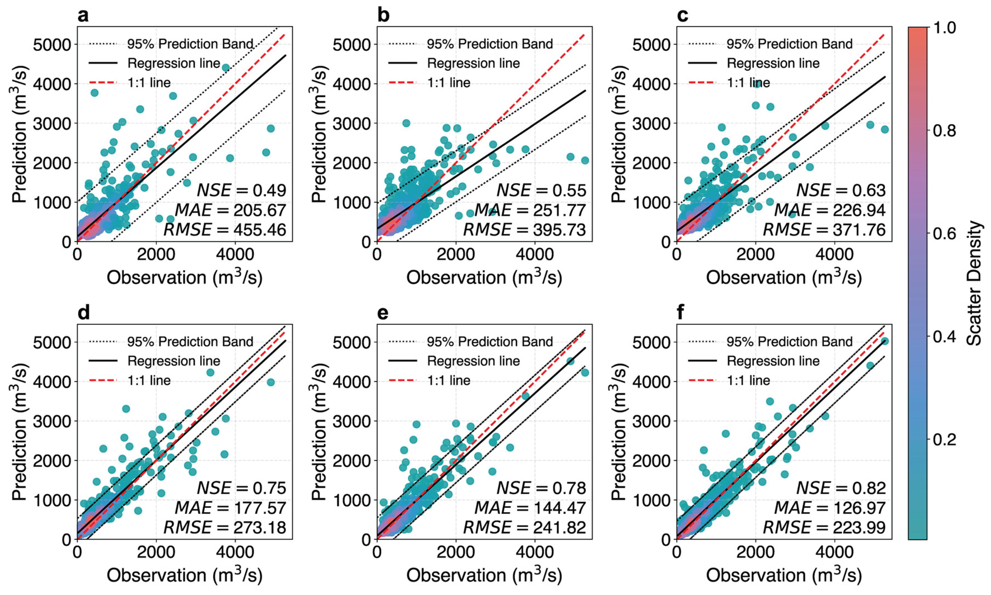
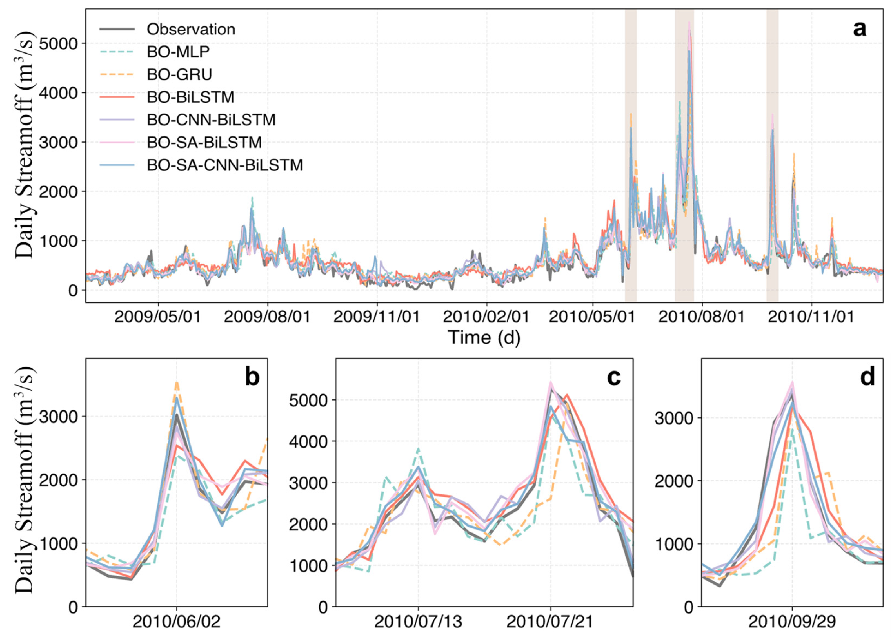
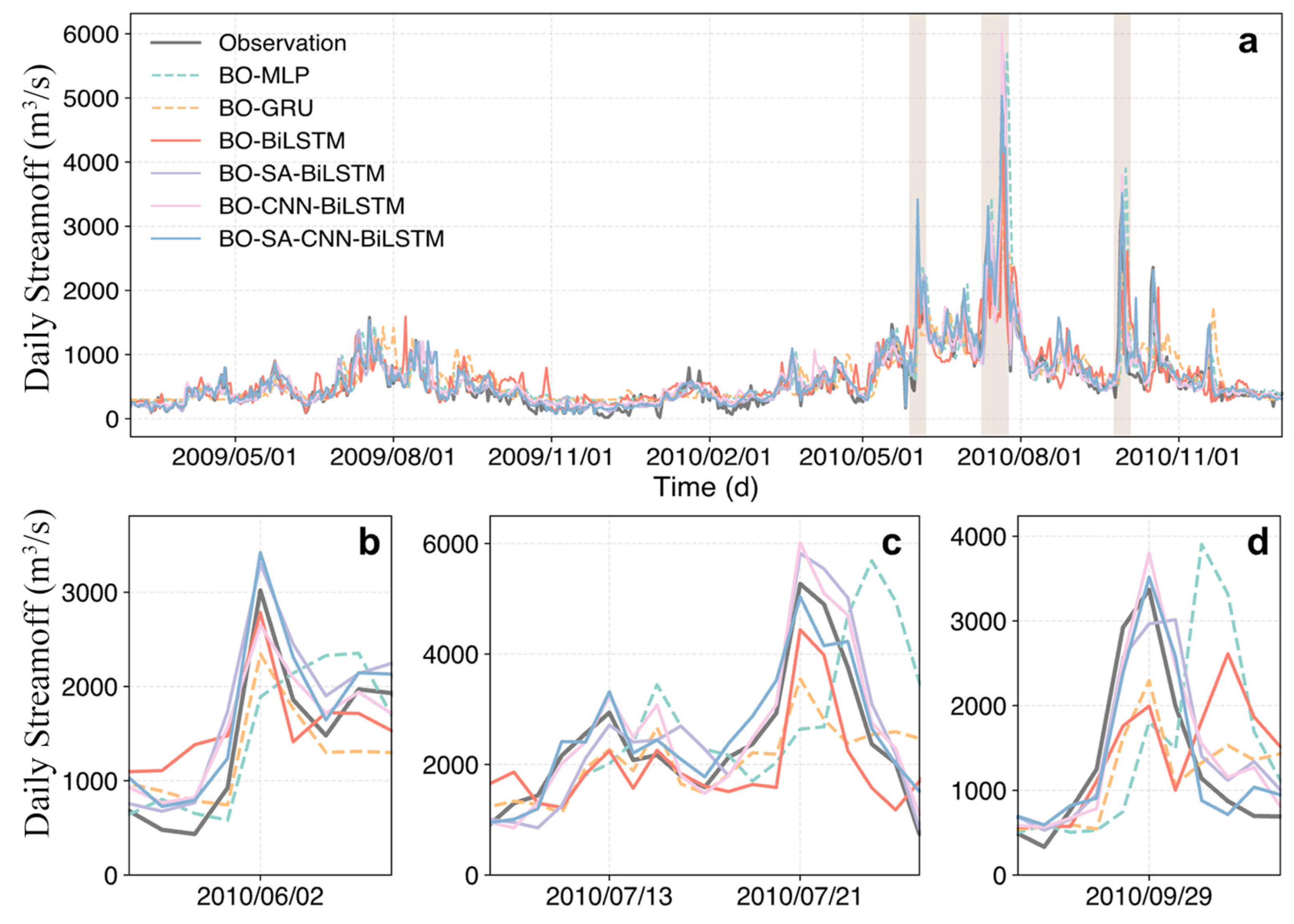
3.1. Model Performance Evaluation
3.2. Flood Event Performance Analysis
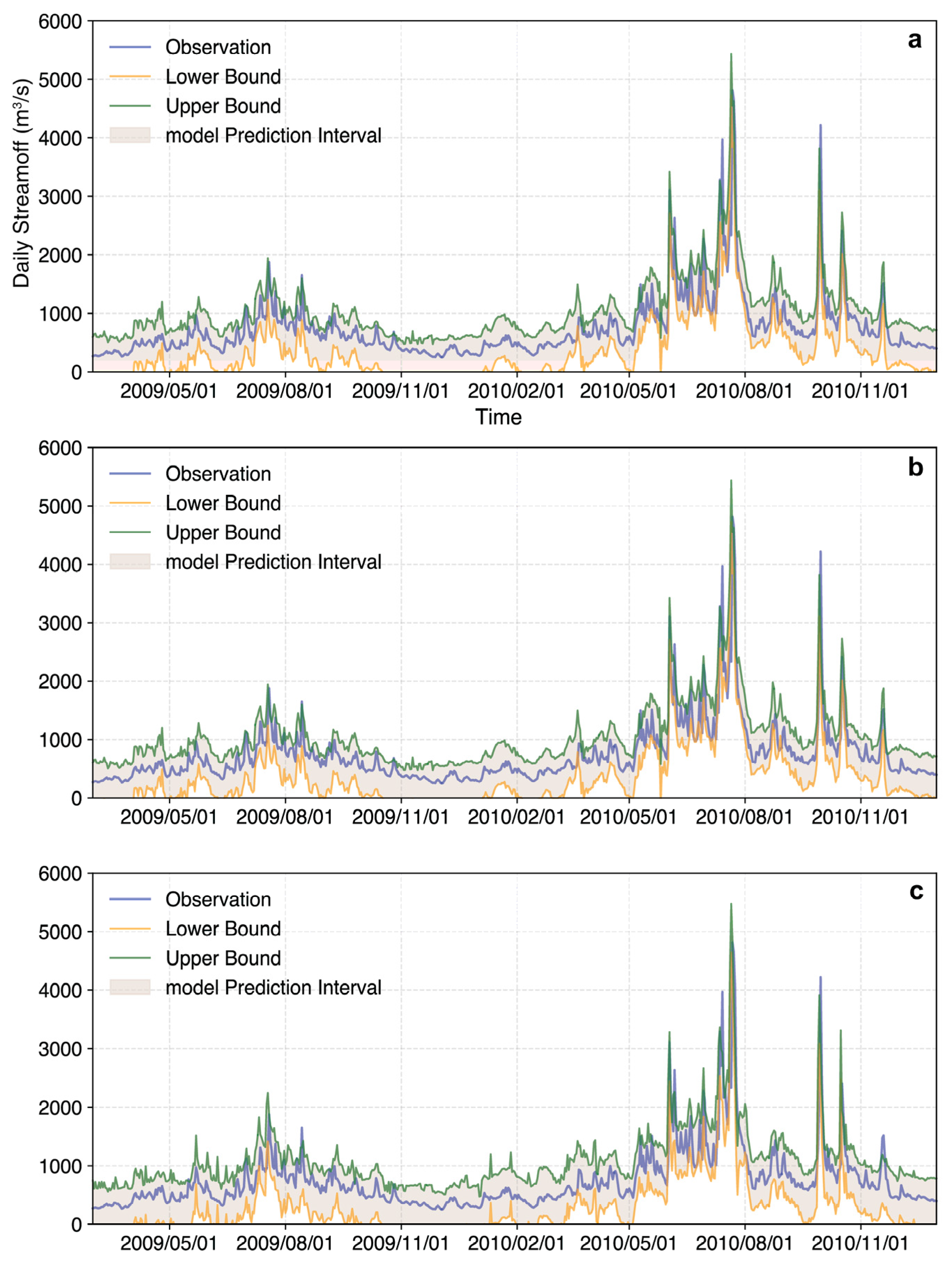
3.3. Interval Prediction of Daily Streamflow for Different Lead Times
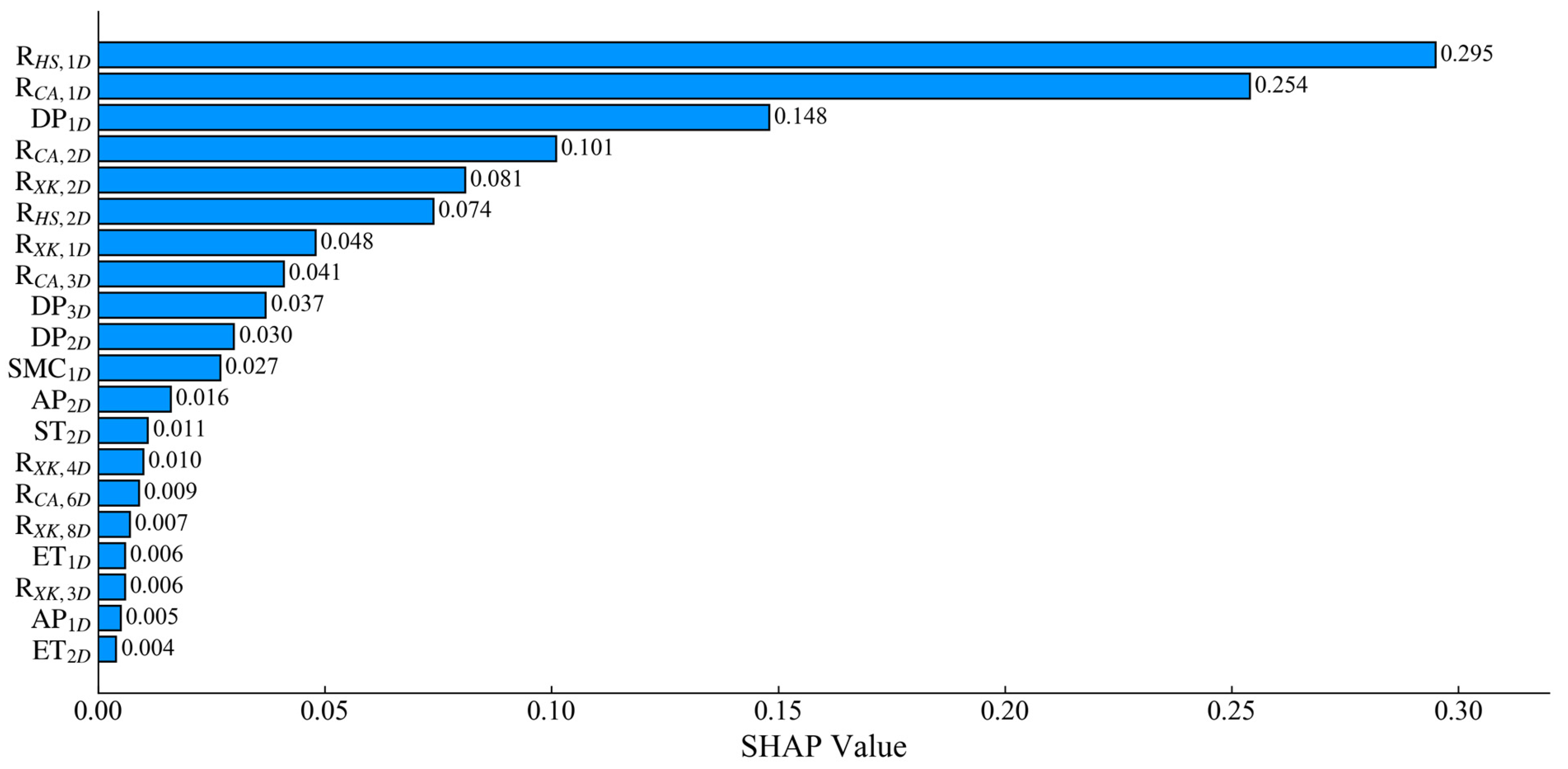
3.4. Feature Importance
3.5. Research Gaps and Future Work
4. Conclusions
Supplementary Materials
Author Contributions
Funding
Data Availability Statement
Conflicts of Interest
References
- Granata, F.; Di Nunno, F. Neuroforecasting of Daily Streamflows in the UK for Short- and Medium-Term Horizons: A Novel Insight. J. Hydrol. 2023, 624, 22. [Google Scholar] [CrossRef]
- Hapuarachchi, H.A.P.; Bari, M.A.; Kabir, A.; Hasan, M.M.; Woldemeskel, F.M.; Gamage, N.; Sunter, P.D.; Zhang, X.S.; Robertson, D.E.; Bennett, J.C.; et al. Development of a National 7-Day Ensemble Streamflow Forecasting Service for Australia. Hydrol. Earth Syst. Sci. 2022, 26, 4801–4821. [Google Scholar] [CrossRef]
- Matrenin, P.; Safaraliev, M.; Dmitriev, S.; Kokin, S.; Eshchanov, B.; Rusina, A. Adaptive Ensemble Models for Medium-Term Forecasting of Water Inflow When Planning Electricity Generation under Climate Change. Energy Rep. 2022, 8, 439–447. [Google Scholar] [CrossRef]
- Zhang, X.; Peng, Y.; Zhang, C.; Wang, B. Are Hybrid Models Integrated with Data Preprocessing Techniques Suitable for Monthly Streamflow Forecasting? Some Experiment Evidences. J. Hydrol. 2015, 530, 137–152. [Google Scholar] [CrossRef]
- Kratzert, F.; Klotz, D.; Brenner, C.; Schulz, K.; Herrnegger, M. Rainfall–Runoff Modelling Using Long Short-Term Memory (Lstm) Networks. Hydrol. Earth Syst. Sci. 2018, 22, 6005–6022. [Google Scholar] [CrossRef]
- Arnold, J.G.; Srinivasan, R.; Muttiah, R.S.; Williams, J.R. Large Area Hydrologic Modeling and Assessment Part I: Model Development. JAWRA J. Am. Water Resour. Assoc. 1998, 34, 73–89. [Google Scholar] [CrossRef]
- Liang, X.; Lettenmaier, D.P.; Wood, E.F.; Burges, S.J. A Simple Hydrologically Based Model of Land Surface Water and Energy Fluxes for General Circulation Models. J. Geophys. Res. Atmos. 1994, 99, 14415–14428. [Google Scholar] [CrossRef]
- Fatichi, S.; Vivoni, E.R.; Ogden, F.L.; Ivanov, V.Y.; Mirus, B.; Gochis, D.; Downer, C.W.; Camporese, M.; Davison, J.H.; Ebel, B.; et al. An Overview of Current Applications, Challenges, and Future Trends in Distributed Process-Based Models in Hydrology. J. Hydrol. 2016, 537, 45–60. [Google Scholar] [CrossRef]
- Shen, C.P.; Appling, A.P.; Gentine, P.; Bandai, T.; Gupta, H.; Tartakovsky, A.; Baity-Jesi, M.; Fenicia, F.; Kifer, D.; Li, L.; et al. Differentiable Modelling to Unify Machine Learning and Physical Models for Geosciences. Nat. Rev. Earth Environ. 2018, 4, 552–567. [Google Scholar] [CrossRef]
- Freire, P.K.D.M.; Santos, C.A.G.; da Silva, G.B.L. Analysis of the Use of Discrete Wavelet Transforms Coupled with Ann for Short-Term Streamflow Forecasting. Appl. Soft Comput. 2019, 80, 494–505. [Google Scholar] [CrossRef]
- Dehghani, A.; Moazam, H.M.Z.H.; Mortazavizadeh, F.; Ranjbar, V.; Mirzaei, M.; Mortezavi, S.; Ng, J.L.; Dehghani, A. Comparative Evaluation of LSTM, CNN, and ConvLSTMfor Hourly Short-Term Streamflow Forecasting Using Deep Learning Approaches. Ecol. Inform. 2023, 75, 12. [Google Scholar] [CrossRef]
- Wagena, M.B.; Goering, D.; Collick, A.S.; Bock, E.; Fuka, D.R.; Buda, A.; Easton, Z.M. Comparison of Short-Term Streamflow Forecasting Using Stochastic Time Series, Neural Networks, Process-Based, and Bayesian Models. Environ. Model. Softw. 2020, 126, 10. [Google Scholar] [CrossRef]
- Chen, Y.Q.; Niu, J.; Sun, Y.Q.; Liu, Q.; Li, S.; Li, P.; Sun, L.Q.; Li, Q.L. Study on Streamflow Response to Land Use Change over the Upper Reaches of Zhanghe Reservoir in the Yangtze River Basin. Geosci. Lett. 2020, 7, 12. [Google Scholar] [CrossRef]
- Mohammed Ji, B.G. Streamflow Modeling under the Impact of Climate Change. (Case Study of Dabus River Sub-Basin, Ethiopia). Topology 2020, 12, 7. [Google Scholar]
- Williams, A.P.; Livneh, B.; McKinnon, K.A.; Hansen, W.D.; Mankin, J.S.; Cook, B.I.; Smerdon, J.E.; Varuolo-Clarke, A.M.; Bjarke, N.R.; Juang, C.S.; et al. Growing Impact of Wildfire on Western Us Water Supply. Proc. Natl. Acad. Sci. USA 2022, 119, 8. [Google Scholar] [CrossRef]
- Huang, H.; Feng, G.; Cao, Y.; Feng, G.; Dai, Z.; Tian, P.; Wei, J.; Cai, X. Simulation and Driving Factor Analysis of Satellite-Observed Terrestrial Water Storage Anomaly in the Pearl River Basin Using Deep Learning. Remote Sens. 2023, 15, 3983. [Google Scholar] [CrossRef]
- Ahmed, Y.; Al-Faraj, F.; Scholz, M.; Soliman, A. Assessment of Upstream Human Intervention Coupled with Climate Change Impact for a Transboundary River Flow Regime: Nile River Basin. Water Resour. Manag. 2019, 33, 2485–2500. [Google Scholar] [CrossRef]
- Yin, H.; Guo, Z.; Zhang, X.; Chen, J.; Zhang, Y. Rr-Former: Rainfall-Runoff Modeling Based on Transformer. J. Hydrol. 2022, 609, 127781. [Google Scholar] [CrossRef]
- Awchi, T.A. River Discharges Forecasting in Northern Iraq Using Different Ann Techniques. Water Resour. Manag. 2014, 28, 801–814. [Google Scholar] [CrossRef]
- Fidal, J.; Kjeldsen, T.R. Accounting for Soil Moisture in Rainfall-Runoff modelling of Urban Areas. J. Hydrol. 2020, 589, 125122. [Google Scholar] [CrossRef]
- Malakoutian, M.M.A.; Samaei, S.Y.; Khaksar, M.; Malakoutian, Y. A Prediction of Future Flows of Ephemeral Rivers by Using Stochastic Modeling (Ar Autoregressive Modeling). Sustain. Oper. Comput. 2022, 3, 330–335. [Google Scholar] [CrossRef]
- Li, P.; Zhang, J.; Krebs, P. Prediction of Flow Based on a CNN-LSTM Combined Deep Learning Approach. Water 2022, 14, 993. [Google Scholar] [CrossRef]
- Ghimire, S.; Yaseen, Z.M.; Farooque, A.A.; Deo, R.C.; Zhang, J.; Tao, X. Streamflow Prediction Using an Integrated Methodology Based on Convolutional Neural Network and Long Short-Term Memory Networks. Sci. Rep. 2021, 11, 17497. [Google Scholar] [CrossRef] [PubMed]
- Zhou, F.; Chen, Y.; Liu, J. Application of a New Hybrid Deep Learning Model That Considers Temporal and Feature Dependencies in Rainfall–Runoff Simulation. Remote Sens. 2023, 15, 1395. [Google Scholar] [CrossRef]
- Ghaith, M.; Siam, A.; Li, Z.; El-Dakhakhni, W. Hybrid Hydrological Data-Driven Approach for Daily Streamflow Forecasting. J. Hydrol. Eng. 2020, 25, 9. [Google Scholar] [CrossRef]
- Lundberg, S.M.; Lee, S.I. A Unified Approach to Interpreting Model Predictions. Adv. Neural Inf. Process. Syst. 2017, 30, 10. [Google Scholar]
- Zhao, Z.; Huang, H.; Wang, J.; Feng, G.; Li, L.; Sun, T.; Li, Y.; Wei, J.; Cai, X. Impacts of the Grain for Green Project on Soil Moisture in the Yellow River Basin, China. Hydrol. Process. 2025, 39, e70112. [Google Scholar] [CrossRef]
- Tulio Ribeiro, M.; Singh, S.; Guestrin, C. “Why Should I Trust You?”: Explaining the Predictions of Any Classifier. arXiv 2016, arXiv:1602.04938. [Google Scholar]
- Tiwari Dk, T.N.R. Geomorphology-Wavelet Based Approach to Rainfall Runoff Modeling for Data Scarce Semi-Arid Regions, Kolar River Catchment, India. J. Eng. Res. 2022, 10, 29–40. [Google Scholar] [CrossRef]
- Wu, Z.Y.; Feng, H.H.; He, H.; Zhou, J.H.; Zhang, Y.L. Evaluation of Soil Moisture Climatology and Anomaly Components Derived from Era5-Land and Gldas-2.1 in China. Water Resour. Manag. 2021, 35, 629–643. [Google Scholar] [CrossRef]
- Reshef, D.N.; Reshef, Y.A.; Finucane, H.K.; Grossman, S.R.; McVean, G.; Turnbaugh, P.J.; Lander, E.S.; Mitzenmacher, M.; Sabeti, P.C. Detecting Novel Associations in Large Data Sets. Science 2011, 334, 1518–1524. [Google Scholar] [CrossRef] [PubMed]
- Murtagh, F. Multilayer Perceptrons for Classification and Regression. Neurocomputing 1991, 2, 183–197. [Google Scholar] [CrossRef]
- Hasan, M.M.; Nilay, M.S.M.; Jibon, N.H.; Rahman, R.M. Lulc Changes to Riverine Flooding: A Case Study on the Jamuna River, Bangladesh Using the Multilayer Perceptron Model. Results Eng. 2023, 18, 101079. [Google Scholar] [CrossRef]
- Granata, F.; Di Nunno, F.; Pham, Q.B. A Novel Additive Regression Model for Streamflow Forecasting in German Rivers. Results Eng. 2024, 22, 102104. [Google Scholar] [CrossRef]
- Sammen, S.S.; Ehteram, M.; Abba, S.I.; Abdulkadir, R.A.; Ahmed, A.N.; El-Shafie, A. A New Soft Computing Model for Daily Streamflow Forecasting. Stoch. Environ. Res. Risk Assess. 2021, 35, 2479–2491. [Google Scholar] [CrossRef]
- Köyceğiz, C.; Büyükyıldız, M. Estimation of Streamflow Using Different Artificial Neural Network Models. Osman. Korkut Ata Üniv. Fen Bilim. Enst. Derg. 2022, 5, 1141–1154. [Google Scholar] [CrossRef]
- Wang, K.; Ma, C.; Qiao, Y.; Lu, X.; Hao, W.; Dong, S. A Hybrid Deep Learning Model with 1DCNN-LSTM-Attention Networks for Short-Term Traffic Flow Prediction. Phys. A Stat. Mech. Its Appl. 2021, 583, 126293. [Google Scholar] [CrossRef]
- Xie, Y.; Sun, W.; Ren, M.; Chen, S.; Huang, Z.; Pan, X. Stacking Ensemble Learning Models for Daily Runoff Prediction Using 1d and 2d CNNs. Expert Syst. Appl. 2023, 217, 119469. [Google Scholar] [CrossRef]
- Hochreiter, S.; Schmidhuber, J. Long Short-Term Memory. Neural Comput. 1997, 9, 1735–1780. [Google Scholar] [CrossRef]
- Sathi, K.A.; Hosain, M.K.; Hossain, M.A.; Kouzani, A.Z. Attention-Assisted Hybrid 1D CNN-BiLSTM Model for Predicting Electric Field Induced by Transcranial Magnetic Stimulation Coil. Sci. Rep. 2023, 13, 2494. [Google Scholar] [CrossRef]
- Srivastava, R.; Mittal, V. Adaw: Age Decay Accuracy Weighted Ensemble Method for Drifting Data Stream Mining. Intell. Data Anal. 2021, 25, 1131–1152. [Google Scholar] [CrossRef]
- Loshchilov, I.; Hutter, F. Decoupled Weight Decay Regularization. arXiv 2017, arXiv:1711.05101. [Google Scholar]
- Frazier, P.I. A Tutorial on Bayesian Optimization. arXiv 2018, arXiv:1807.02811. [Google Scholar]
- Akiba, T.; Sano, S.; Yanase, T.; Ohta, T.; Koyama, M. Optuna: A Next-Generation Hyperparameter Optimization Framework. arXiv 2019, arXiv:1907.10902. [Google Scholar]
- Diebold, F.X.; Mariano, R.S. Comparing Predictive Accuracy (Reprinted). J. Bus. Econ. Stat. 2002, 20, 134–144. [Google Scholar] [CrossRef]
- Mangini, W.; Viglione, A.; Hall, J.; Hundecha, Y.; Ceola, S.; Montanari, A.; Rogger, M.; Salinas, J.L.; Borzì, I.; Parajka, J. Detection of Trends in Magnitude and Frequency of Flood Peaks across Europe. Hydrol. Sci. J. 2018, 63, 493–512. [Google Scholar] [CrossRef]
- Terrell Gr, S.D.W. Variable Kernel Density Estimation. Ann. Stat. 1992, 20, 1236–1265. [Google Scholar] [CrossRef]
- Aumann, R.J.; Hart, S. Handbook of Game Theory with Economic Applications; Elsevier: Amsterdam, The Netherlands, 1992; Volume 2. [Google Scholar]
- Liu, H.; Motoda, H. Feature Selection for Knowledge Discovery and Data Mining; Springer Science & Business Media: New York, NY, USA, 2012; Volume 454. [Google Scholar]
- Brochu, E.; Cora, V.M.; de Freitas, N. A Tutorial on Bayesian Optimization of Expensive Cost Functions, with Application to Active User Modeling and Hierarchical Reinforcement Learning. arXiv 2010, arXiv:1012.2599. [Google Scholar]
- Snoek, J.; Larochelle, H.; Adams, R.P. Practical Bayesian Optimization of Machine Learning Algorithms. Adv. Neural Inf. Process. Syst. 2012, 25. [Google Scholar]
- Shahriari, B.; Swersky, K.; Wang, Z.Y.; Adams, R.P.; de Freitas, N. Taking the Human out of the Loop: A Review of Bayesian Optimization. Proc. IEEE 2016, 104, 148–175. [Google Scholar] [CrossRef]
- Jones, D.R.; Schonlau, M.; Welch, W.J. Efficient Global Optimization of Expensive Black-Box Functions. J. Glob. Optim. 1998, 13, 455–492. [Google Scholar] [CrossRef]
- Silverman, B.W. Density Estimation for Statistics and Data Analysis; Routledge: London, UK, 2018. [Google Scholar]
- Abebe, N.A.; Ogden, F.L.; Pradhan, N.R. Sensitivity and Uncertainty Analysis of the Conceptual Hbv Rainfall–Runoff Model: Implications for Parameter Estimation. J. Hydrol. 2010, 389, 301–310. [Google Scholar] [CrossRef]


| Station Name | Station Code | Water Resources Zone IV | Catchment Area (km2) | Mean Annual Streamflow (billion m3) |
|---|---|---|---|---|
| Chaoan | 81,500,650 | lower reaches of the Hanjiang River | 29,077 | 22.580 |
| Hengshan | 81,500,360 | Meijiang River | 12,624 | 9.698 |
| Xikou | 81,503,050 | Tingjiang River | 9228 | 8.197 |
| Station Name | Station Code | Station Coordinates |
|---|---|---|
| Changting | 58,911 | 25.51° N, 116.22° E |
| Shanghang | 58,918 | 25.03° N, 116.25° E |
| Yongding | 59,113 | 24.44° N, 116.43° E |
| Dabu | 59,116 | 24.20° N, 116.42° E |
| Meixian | 59,117 | 24.16° N, 116.06° E |
| Wuhua | 59,303 | 23.56° N, 115.46° E |
| Number | Variable | Unit | Data Source |
|---|---|---|---|
| F1 | Daily precipitation | mm | Dataset of daily values of surface climate data in China (V3.0) |
| F2 | Average daily relative humidity | % | |
| F3 | Daily average surface temperature | °C | |
| F4 | Daily maximum surface temperature | °C | |
| F5 | Daily minimum surface temperature | °C | |
| F6 | Average daily temperature | °C | |
| F7 | Daily maximum temperature | °C | |
| F8 | Daily lowest temperature | °C | |
| F9 | Daily average air pressure | hPa | |
| F10 | Daily maximum air pressure | hPa | |
| F11 | Daily minimum pressure | hPa | |
| F12 | Sunshine hours | h | |
| F13 | Average wind speed | m s−1 | |
| F14 | Maximum wind speed | m s−1 | |
| F15 | Daily evapotranspiration | mm | |
| F16 | Soil water content (0–7 cm) | m3 m−3 | ERA5-Land |
| F17 | Soil water content (7–28 cm) | m3 m−3 | |
| F18 | Soil water content (28–100 cm) | m3 m−3 | |
| F19 | Soil water content (100–289 cm) | m3 m−3 | |
| F20 | Average daily streamflow at Hengshan Station | m3 s−1 | Hanjiang River Basin Management Bureau |
| F21 | Average daily streamflow at Xikou Station | m3 s−1 | |
| F22 | Average daily streamflow at Chaoan Station | m3 s−1 |
| Number | Variable | Acronyms | MIC |
|---|---|---|---|
| F1 | Daily precipitation | DP | 0.44 |
| F2 | Daily average relative humidity | RH | 0.19 |
| F5 | Daily minimum surface temperature | ST | 0.33 |
| F8 | Daily minimum air temperature | T | 0.32 |
| F9 | Daily average air pressure | AP | 0.31 |
| F15 | Daily evapotranspiration | ET | 0.22 |
| F17 | Soil water content | SMC | 0.48 |
| F20 | Average daily streamflow at Hengshan Station | RHS | 0.51 |
| F21 | Average daily streamflow at Xikou Station | RXK | 0.36 |
| F22 | Average daily streamflow at Chaoan Station | RCA | 1.00 |
| Forecast Period | Base Model | DM Value | p |
|---|---|---|---|
| 1d | MLP | 6.71 | 4.09 × 10⁻¹⁰ |
| GRU | 4.41 | 1.21 × 10⁻⁵ | |
| BiLSTM | 3.13 | 1.82 × 10⁻⁴ | |
| CNN-BiLSTM | 2.44 | 6.08 × 10⁻³ | |
| SA-BiLSTM | 2.59 | 9.71 × 10⁻⁴ | |
| 3d | MLP | 6.35 | 3.92 × 10⁻¹⁰ |
| GRU | 5.98 | 3.64 × 10⁻⁹ | |
| BiLSTM | 4.21 | 2.90 × 10⁻⁵ | |
| CNN-BiLSTM | 2.14 | 3.27 × 10⁻³ | |
| SA-BiLSTM | 2.46 | 1.43 × 10⁻³ | |
| 5d | MLP | 5.34 | 1.30 × 10⁻⁷ |
| GRU | 5.16 | 3.33 × 10⁻⁷ | |
| BiLSTM | 5.02 | 6.57 × 10⁻⁷ | |
| CNN-BiLSTM | 2.18 | 2.95 × 10⁻³ | |
| SA-BiLSTM | 3.65 | 2.83 × 10⁻⁴ |
| Confidence Interval | Forecast Period | PICP | PINAW |
|---|---|---|---|
| 80% | 1d | 82.71% | 8.54% |
| 3d | 80.92% | 9.27% | |
| 5d | 84.20% | 10.33% | |
| 85% | 1d | 86.29% | 10.51% |
| 3d | 85.84% | 12.30% | |
| 5d | 88.52% | 13.97% | |
| 90% | 1d | 92.55% | 13.58% |
| 3d | 93.29% | 15.67% | |
| 5d | 93.00% | 18.39% | |
| 95% | 1d | 96.13% | 20.25% |
| 3d | 97.17% | 23.96% | |
| 5d | 96.57% | 28.24% |
Disclaimer/Publisher’s Note: The statements, opinions and data contained in all publications are solely those of the individual author(s) and contributor(s) and not of MDPI and/or the editor(s). MDPI and/or the editor(s) disclaim responsibility for any injury to people or property resulting from any ideas, methods, instructions or products referred to in the content. |
© 2025 by the authors. Licensee MDPI, Basel, Switzerland. This article is an open access article distributed under the terms and conditions of the Creative Commons Attribution (CC BY) license (https://creativecommons.org/licenses/by/4.0/).
Share and Cite
Huang, J.; Chen, J.; Huang, H.; Cai, X. Deep Learning-Based Daily Streamflow Prediction Model for the Hanjiang River Basin. Hydrology 2025, 12, 168. https://doi.org/10.3390/hydrology12070168
Huang J, Chen J, Huang H, Cai X. Deep Learning-Based Daily Streamflow Prediction Model for the Hanjiang River Basin. Hydrology. 2025; 12(7):168. https://doi.org/10.3390/hydrology12070168
Chicago/Turabian StyleHuang, Jianze, Jialang Chen, Haijun Huang, and Xitian Cai. 2025. "Deep Learning-Based Daily Streamflow Prediction Model for the Hanjiang River Basin" Hydrology 12, no. 7: 168. https://doi.org/10.3390/hydrology12070168
APA StyleHuang, J., Chen, J., Huang, H., & Cai, X. (2025). Deep Learning-Based Daily Streamflow Prediction Model for the Hanjiang River Basin. Hydrology, 12(7), 168. https://doi.org/10.3390/hydrology12070168