Abstract
The bubble shape influences the transfer of momentum and heat/mass between the bubble and the surrounding fluid as well as the flow field around the bubble. The shape is determined by the interaction of the fluid field in the bubble, the physics on the surface, and the surrounding flow field. It is well known that contaminations can disturb the surface physics so that the bubble shape can be influenced. Indeed, an influence of sodium chloride (NaCl) on the hydrodynamics of bubbly flows was shown for air/water systems in previous studies. The aim of the present work is to investigate if, and to what extent, the NaCl concentration affects the bubble shape in bubble columns. For this purpose, several experiments at the Helmholtz-Zentrum Dresden-Rossendorf and at the pilot-scale bubble column at the Politecnico di Milano are evaluated. The experiments were executed independently from each other and were evaluated with different methods. All experiments show that the bubble shape is not distinctly affected in the examined concentration range from 0 to 1 M NaCl, which is in contrast to a previous study on single bubbles. Therefore, the effect of NaCl on the hydrodynamics of bubbly flows is not induced by the bubble shape.
1. Introduction
In multiphase flows, the interface size and its shape are one of the most important modelling parameters. Bubbles, in particular wobbling bubbles, have a very complex interface since many effects determine the bubbles shape. In pure conditions, the bubble shape can be estimated by using, for example, the Reynolds, Eötvös, and Morton number (e.g., [1]). Indeed, this estimation is only valid for single bubbles in quiescent flows. In turbulent bubbly flows, like the flow field found in bubble columns, the surrounding turbulence can affect the bubble shape. However, the influence of the turbulent flow field that is usually found in bubble columns is rather small at low to medium void fractions [2].
The situation is changed when the fluid contains contaminations. Different types of contaminations exist, which can be classified as weak and strong contaminations. Weak and strong refers at this point on the effect on the bubbles. Contaminations change the surface tension, which is in principle included in the above-mentioned dimensionless numbers. However, due to the slip velocity of bubbles, the contaminations are dragged to the bubble tail so that the concentration on the surface is not homogenous. This gradient in the surface tension induces a flow that can be strong enough to counteract the drag-induced flow on the bubble surface. As a result, the bubble can behave like a rigid sphere or a bubble with a stagnant cap [3,4]. This behavior is also determined by the absorption/desorption kinetics of the surfactant on the interface, which greatly depends on the mixture of added surfactants [5].
Certainly, the contaminations change fluid dynamics of the bubble drastically, which was shown experimentally [6,7] and theoretically [8]. Besides this, also the bubble shape [9,10] and the behavior regarding coalescence and break-up [11] is influenced. These three, usually connected, effects can have a distinct influence on the general hydrodynamics of bubbly flows. That the bubble coalescence is suppressed by adding electrolytes is widely accepted and is not part of the present work. The effect of electrolytes on the bubble shape and hydrodynamics, in respect to the drag and lift force, is however, not yet fully understood.
The application of contaminated surfaces is wide, from bubble columns [12,13,14], and Taylor bubbles in micro channels [15], to deep-sea applications [16]. One focus is on the changing mass transfer when surfactants are added [10,17]. In recent years, the effect of surfactants has also been studied numerically [18,19]. Since the present work is focusing on electrolytes, specifically NaCl, added to water, a particular application is also the emergency cooling of nuclear power reactors with seawater as was done in the Daiichi accident near Fukushima in 2011 after an earthquake (e.g., [20]). In general, also a link to previous deep-sea studies could be drawn [16,21,22,23]. One conclusion out of these studies is that the average bubble rise-velocity is not distinctly affected. However, the standard deviation is smaller when salt is added [16]. This might be connected to an overall suppression of the shape oscillation, which is important for the terminal velocity [9]. Indeed, the conclusion was drawn from a recent study, which investigated single bubbles rising in different salt solutions, that NaCl has a distinct influence on the bubble shape [24].
This influence on the bubble shape in bubble columns when NaCl is added is the focus of the present work. As discussed above, the bubble shape is very strongly connected to the hydrodynamics of bubbly flows and the mass transfer between a gas and liquid phase. Therefore, a better comprehension of the effect of salt can help to improve closure models, which are essential for CFD simulations [25]. Since salt is a contamination that is found regularly in applications, the findings can help to extend baseline models for bubbly flows [26] with which CFD simulations can be used to design and optimize two-phase flow apparatuses. Moreover, the flow in bubble columns is turbulent and bubbles rise in swarms, which can influence the distribution of contaminations on the surface. Therefore, it is not clear which findings that are obtained from single bubbles rising in a quiescent environment can be used in bubble columns.
For this purpose, several experiments at the Helmholtz-Zentrum Dresden-Rossendorf (HDZR) and at the pilot-scale bubble column at the Politecnico di Milano (PoliMi) are evaluated. The following dimensionless numbers are used to describe the problem:
with density difference, the acceleration due to gravitation, the surface tension coefficient, the relative velocity of the bubble, and the dynamic viscosity the. The bubble size, , is defined as the diameter of a sphere with volume equivalent the bubble volume. The major axis, , is defined as the largest extend of the projected bubble and the minor axis, , as the largest extent perpendicular to the major axis [2]. The ratio of both axis is defined as the eccentricity, . With the , , and number from Equation (1)., the bubble shape in most clean, quiescent fluid can be described explicitly [1]. Usually, one number can be calculated from the other with a model, e.g., with a drag correlation, so that not all three are necessary. However, bubble and droplet shapes are often modeled with the product of , which is called as Weber number. Particularly for bubbles, the product , which is called the Tadaki number, is also often used. Since in the present case the Morton number is almost constant, as explained in the following section, we will show only the eccentricity vs. the Eötvös number in the result section. This representation is often used since it is simple and valid for a specific range of similar fluids.
2. Materials and Methods
In the following, the change in the surface tension in N per m due to the added salt is calculated with the fit taken from [27] given in Equation (2):
where S is the salinity in g per kg and T the temperature in Kelvin. The surface tension of pure water is calculated with the IAPWS correlation (IAPWS Release on Surface Tension of Ordinary Water Substance, September 1994) given in Equation (3):
The density and viscosity of the salt solutions were calculated with the NIST database. However, the differences in the surface tension, viscosity and density are minor in the used concentration range. All experiments were conducted in a temperature range between 20 and 25 °C. Due to the large facilities and the relatively high gas volume flows, in which temperatures were not adjusted, this temperature range is acceptable.
2.1. Bubble Column Experiments at Helmholtz-Zentrum Dresden-Rossendorf (HZDR)
The experimental setup consists of a tall bubble column with six holes for needle spargers. To produce different flow regimes, different needle sizes can be placed into the holes. For this purpose, the holes are divided in Group 1 (G1) and Group 2 (G2) (Figure 1). The spargers in G1 and G2 have a separated gas supply. The needle size and gas flow rates used in the present study are given in Table 1. The gas volume flow is ranging from 1.0 to 1.5 L/min at standard conditions, which is equal to 0.3 cm/s and 0.45 cm/s superficial velocity respectively. The filtered airflow per sparger group was controlled by a mass flow controller from OMEGA Engineering GmbH each. Filtered and afterwards deionized water was used to produce a 0.205 M NaCl (analysis quality, 99.9% in mass) solution that is used for all experiments. Every 4 h, the NaCl solution was replaced.
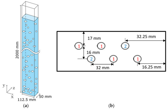
Figure 1.
Dimension of the experimental setup (a) and sparger setup (b) with sparger Group (G) enumeration of the bubble column experiment at HZDR.

Table 1.
Operation points of the bubble column experiment at HZDR.
The bubbly flow was observed from the outside with view on the xy plane (Figure 1). A 240 W LED backlight was placed behind the observation plane so that the shadows of the bubbles were recorded. For recording, the Q-VIT high-speed camera (AOS Technologies AG, Baden Daettwil, Switzerland) from AOS Technologies AG was used. A picture shows the complete column width of 0.1125 m, the complete column depth of 0.05 m, and a height of 0.05 m at y = 1200 mm. The resolution was chosen to be 70 µm per pixel. Every two seconds a picture was recorded; the total measuring time was 30 min. From these pictures, an arbitrary set of pictures was chosen for evaluation by hand.
The bubbles, which were partially overlaid, were segmented by hand; afterwards, an ellipsoidal fit was applied to obtain the bubble shape (Figure 2a). The ellipsoidal fit was afterwards checked and if necessary corrected by hand. This procedure advanced the bubble picking compared to classical methods without the usage of the ellipsoidal fit significantly. We were therefore able to evaluate per measuring point around 4000 bubbles so that we have 32,000 bubbles available in total (Figure 2b).
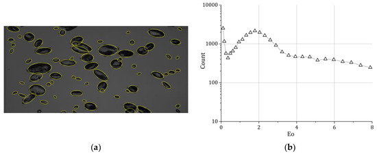
Figure 2.
(a) Result of the ellipsoidal fit; (b) count of the identified bubbles with respect to 0.25 mm large bubble size classes.
2.2. Bubble Plume Experiments at Helmholtz-Zentrum Dresden-Rossendorf
Additionally, bubbles were evaluated in a bubble plume setup (Figure 3). The bubble plume setup is characterized by a central gassing at the bottom of the bubble column. Again, the sparger was separated into two Groups and several setups were measured (Table 2). The gas flow was significantly larger and was operated up to 4.8 L/min. Despite the maximal superficial velocity of 0.64 cm/s (referred to the bubble column cross section) being in the range of the bubble column setup, the bubbly flow is much denser due to the central gassing. The 0.45 M NaCl solution, which is used for all bubble plume experiments, was produced in the same way as the solution for the bubble column and was changed every 4 h, too.
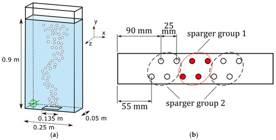
Figure 3.
Experimental setup (a) and sparger setup (b) of the bubble plume experiment at HZDR.
Table 2.
Operation points of the bubble column experiment at HZDR.
Since the bubbly flow is denser compared to the bubble column experiments, the evaluation of the bubbles from one picture is not working anymore. The bubbles rise in swarms so that many bubbles are overlaid by others. To overcome this problem, the bubbles are evaluated at different frames recorded from the high-speed camera. Bubbles that are overlaid in the first frame are evaluated five frames later; if a bubble is still overlaid, it is evaluated 10 frames later [28] (Figure 4). Great care was taken not to evaluate a bubble twice. For the present setup, the high-speed camera recorded every two seconds a set of 10 pictures with 250 frames per second. The total measuring time was again 30 min. Sets for evaluation were chosen arbitrary.
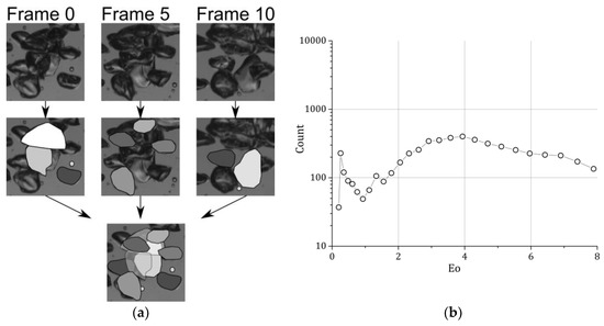
Figure 4.
Evaluation method for the bubble plume experiments [24] (a) and the number distribution of the evaluated bubbles (b).
2.3. Experiments at Politecnico di Milano
The experimental facility (Figure 5) is a non-pressurized vertical pipe made of Plexiglas® (AD Plast s.r.l., Milano, Italy) with dc = 0.24 m and Hc = 5.3 m. A pressure reducer controls the pressure upstream from the pressure calibrated rotameters (1) and (2), used to measure the gas flow rate (accuracy ± 2% f.s.v., E5-2600/h, manufactured by ASA, Italy). A pump, controlled by a bypass valve, provides water recirculation, and a rotameter (3) measures the liquid flowrate (accuracy ± 1.5% f.s.v., G6-3100/39, manufactured by ASA, Italy).
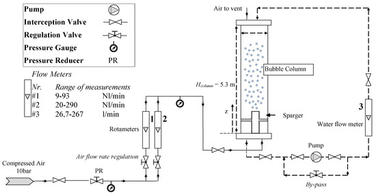
Figure 5.
Experimental setup of the bubble column at the Politecnico di Milano.
The experimental facility was equipped with boxes for flow visualization (see [29,30]). The values of gas density (used to compute the gas superficial velocity) are based upon the operating conditions existing at the column mid-point (computed by using the ideal gas law) [31]. The gas sparger is a spider-sparger with hole diameters do = 2–4 mm. It has six arms made of 0.12 m diameter stainless steel tubes soldered to a center cylinder [30]. The sparger was installed with the six holes located on the side of each arm facing upward. The gas and liquid temperatures have been checked and maintained constant at room temperature during all the experiments (295 ± 1 K); a survey on the influence of the operating conditions was proposed by different reviews [32,33] and is not repeated here. Filtered air has been used as the gaseous phase in all the experiments; the air-cleaning line consists of filters (mechanical and activated carbon) and condensation drying unit. The liquid phase is deionized water with different contents of sodium chloride (kitchen quality, NaCl 98.52% in mass) as electrolyte. During the experimentation, great care has been taken to ensure that the bubble column has been always clean to minimize any contamination that might affect the results (the system has been previously flushed several times with purified water to remove contaminants and to avoid the presence of additional surfactants). A discussion concerning the influence of the liquid phase and salt quality was discussed by Ruzicka et al. [13] and Orvalho et al. [14].
The influence of NaCl over the bubble column fluid dynamics has been tested in the batch mode (UL = 0 cm/s). Five gas superficial velocities have been analyzed, namely: UG = 0.37 cm/s, 0.74 cm/s, 1.11 cm/s, 1.49 cm/s, and 1.88 cm/s, and five NaCl concentrations have been analyzed, namely: 0.1, 0.4, 0.7, 0.84, and 1.0 M. Since we found no influence of the superficial gas velocity on the bubble shape in the used range, the bubble shape is averaged over the superficial velocities. As a result, around 2000 bubbles were evaluated per concentration.
Image analysis has been used to obtain the bubble size distributions and shape data. The photos have been obtained using a NIKON D5000 camera (f/3.5; 1/1600s; ISO400; 4288 × 2848 pixels; spatial resolution approximately 70 µm/Pixel, (Nikon, Tokyo, Japan) using the back light method (500 W halogen lamp as light source). The flow was observed through flow visualization boxes in order to get undistorted images from the round bubble column. Certainly, some refraction problems may still arise—the refraction index of the Plexiglas® pipe wall (equal to 1.48) is different from that of water (equal to 1.33)—but this effect has been proved to be negligible [34]. Images have been acquired at h = 2.4 m from the sparger (which corresponds to the developed region of the two-phase flow [22]). Bubbles were tracked by hand from the images.
Spherical and ellipsoidal bubbles are approximated and reconstructed by using ellipses [22]. For this purpose, sampling points on the outline of the projected bubble were selected by hand (Figure 6a. Using the hypothesis of the axi-symmetric bubble, the spherical equivalent diameter is calculated with the rotational volume of the two dimensional ellipse.
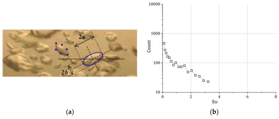
Figure 6.
Sample photos 2.4 m above the sparger for UG = 0.37 cm/s (a) and the number distribution of the evaluated bubbles (b).
The discussion concerning the errors made during the bubble shape estimation due to the handpicked points was proposed in ref. [22]; in addition, the reader may refer to [30,34] for a complete discussion concerning uncertainties in image analysis. The number of bubbles to be sampled to achieve a reliable bubble size distribution (BSD) is a matter of discussion in the literature: various studies sampled different numbers of bubbles, and in this study, for each case, at least several hundred bubbles have been selected using two (or more) photos (Figure 6b).
2.4. Error Analysis
Despite the measuring techniques being relatively simple, the errors that can occur are manifold. First, the bubbles are evaluated by hand, which includes an error that is hard to assess. However, from tests with more than five persons evaluating the same data, almost the same averaged results and standard deviations were obtained with negligible differences. Therefore, we assume that the human error is negligible.
Conventional, non-telecentric lenses were used to record the images of the bubble flow. From test images, the error due to distortion was negligibly small so that this error can be neglected. The perspective error was kept as small as possible in the HZDR experiments by moving the camera 2 m away from the bubble column. In fact, with a depth of the 5 cm, the bubbles in the HZDR experiments at the front or rear wall would appear 3.5% bigger or smaller, respectively, compared to the center. In the Milan experiments, the perspective error was reduced by a smaller depth of focus. Assuming the bubble sizes are homogenously distributed over the depth, the perspective error is nullified when averages are calculated. Nevertheless, the bubble size distribution is always widened by the perspective error.
The bubble size distributions are even more widened by the error due to the projection of wobbling bubbles. Wobbling bubbles of the same volume are projected on the photo sensor in a different size. This error is caused by the elongation of the bubble in different axis due to the wobbling nature and cannot be avoided. However, from the three-dimensional observation of single bubbles, Liu et al. [35] concluded that the average of the projection over time is representing the real bubble volume, which is the same result we obtained from own single bubble experiments. Moreover, Liu et al. [35] confirmed that the assumption of a (averaged) rotational ellipsoid is a good approximation of the averaged bubble shape and represents the averaged bubble volume. At this point, we assume that these findings obtained from single bubble experiments are also valid for bubbly flows in bubble column at lower void fractions. In principle, these assumptions are only valid for the average values. Since we will use the instantaneous bubble size, which is inaccurate due to the projection error, to sort the bubbles in size-bins and average the bubble shape in these bins, bubbles will be sorted in the wrong bins. In addition, bubbles of different sizes have a different wobbling characteristic so that this error is bubble size dependent. Summarizing, the projection error can be interpreted as a complex filter operation that operates in addition to the box filter of the size-bin discretization. Therefore, gradients in diagrams that have the bubble size on the abscissa are usually smoothed out to some extent.
Nevertheless, that these assumptions regarding the averaged values are meaningful will be shown in the following by calculating the superficial gas velocities from the bubble pictures taken with the high-speed camera. To calculate the superficial velocity, the rise velocity of every single bubble over the cross section is needed. To calculate the rise velocity the position of all bubbles at a later time is needed, which was realized by evaluating the bubbles 1/200 s later with the same ellipsoidal method described above for the homogenous bubble column experiments at HZDR (cf. Figure 2). From the known bubble positions in the two consecutive pictures, the velocity of every bubble is obtained by using a tracking algorithm for dilute Particle Tracking Velocimetry (PTV) [36], which was done for the experiments B01, B12, and B03 as examples. Comparing the results with the superficial velocity adjusted at the Mass Flow Controllers (MFC) (OMEGA Engineering, INC., Norwalk, CT, USA) from Omega®, a general error can be estimated, which was quite low for the homogenous HZDR bubble column (Figure 7). The error of the MFCs is given from the manufacturer to be below 1%. By comparing different MFCs designed for different mass flow ranges, the results for the volume flow differed in a range of ±2%. Compared to a rotameter, the differences in the used volume flow range were below 5%.
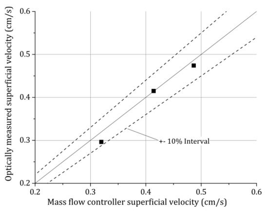
Figure 7.
Comparison of the superficial velocity obtained from optical measurements, which includes the tracking of single bubbles, with the superficial velocity adjusted at the mass flow controllers.
As explained above, the wobbling of the bubbles causes a widened bubble size distribution due to the projection error. Therefore, more bubbles need to be tracked by evaluating the bubble projection compared to three-dimensional measurements. The statistical quality of an averaged value can be quantified with the statistical uncertainty given by , with the standard deviation and the amount of evaluated bubbles. The very large number of several thousand evaluated bubbles results in a relatively low statistical uncertainty for the bubble size (Figure 8a). However, the statistical uncertainty of the eccentricity is still noticeable (Figure 8b).
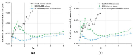
Figure 8.
Statistical uncertainty of the bubble size (a) and the eccentricity (b).
3. Results
In the following, the results are averaged over the volume flow rates since we did not noticed distinct differences between them [2]. Since the focus is on the influence of the NaCl concentration, we only examine the eccentricity, E, with respect to the Eötvös number, Eo. The bubble shape results for different Eo and NaCl concentration are summarized in Figure 9.
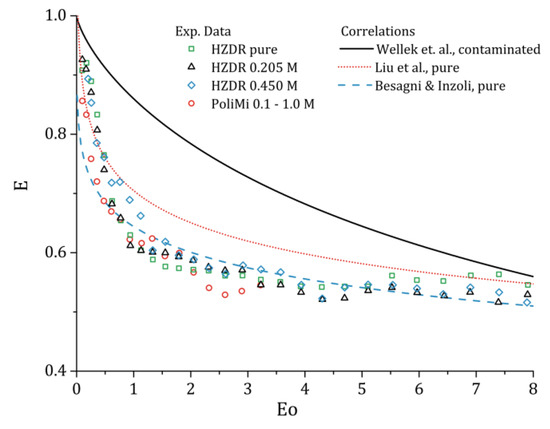
Figure 9.
Bubble shape versus the Eötvös number for different NaCl concentrations. The symbols represent the results of the experiments with the corresponding NaCl concertation, the lines the correlations taken from literature.
For the HZDR experiments, no influence on the averaged bubble shape can be seen. The shape correlation for Eo obtained in purified water [2] is the same as in 0.205 M and 0.450 M NaCl concentrations. Due to a smaller set of evaluated bubbles (cf. Figure 6), the PoliMi results varied randomly around their previously obtained correlation in pure conditions [34] with different NaCl concentrations. However, when the results are averaged over the different concentrations, the results are almost on top of the HZDR results and follow a reasonable smooth curve. Compared to previous measurements, the results follow, with a small offset, the results of Liu et al. [35], which were obtained for single bubbles in purified water, and the results of Besagni & Inzoli [34], which were obtained in a bubble column operated with purified water. The correlation of Wellek et al. [37], which is commonly used for contaminated systems, does not represent the present results.
Since in previous measurements it was observed that the standard deviation of the rise velocity is different when salt is added [16], an evaluation of the bubble shape distribution is interesting. In Figure 10, the number density distribution of the bubble shape obtained in purified conditions and in 0.205 M NaCl is compared for two different bubble size ranges. The purified and the salt experiments were conducted in the same bubble column setup with comparable superficial velocities; the results are again averaged over all volume flow rates. The experiments without salt, which are described in [2], were performed around half a year before the salt measurements. Moreover, many more experiments were evaluated for the purified condition so that better statistics (i.e., smoother curves) are expected. Nevertheless, for bubbles in the range of 2 to 3 mm and in the range of 4 to 5 mm, no distinct differences can be observed by adding salt.
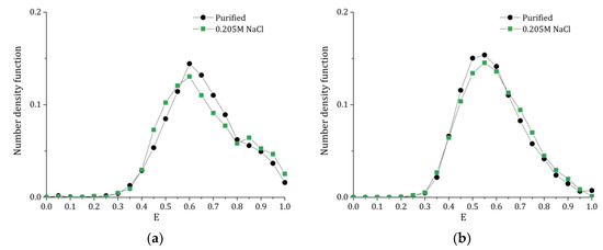
Figure 10.
Number density distribution of the bubble shape for 2 to 3 mm bubbles (a) and 4 to 5 mm bubbles (b).
Finally, the influence of the NaCl concentration on 2.3 mm bubbles is evaluated in Figure 11. In previous experiments, Quinn et al. [24] observed a distinct change in the bubble shape of single bubbles when NaCl is added. To compare their single bubble results to our swarm results, we averaged the bubble shape over bubbles in the interval of 2.2 to 2.4 mm. Again, the results show that we cannot observe a change in the bubble shape when salt is added. The fluctuations of the PoliMi results are interpreted as statistically due to a small set of evaluated bubbles, as discussed above. The results of Quinn et al. [24], which tend with increasing salt concentration to the fully contaminated results described by the Wellek correlation, can therefore be not confirmed in our experiments.
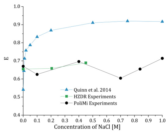
Figure 11.
Bubble shape of 2.3 mm bubbles versus the NaCl concentration obtained at HZDR and PoliMi compared to the results of Quinn et al., 2014 [24].
4. Discussion & Conclusions
From the results conducted independently at HZDR and PoliMi, no change in the bubble size could be observed by adding NaCl to purified water. This is in contrast to the measurements of Quinn et al., 2014 [24], who reported an almost exponential approach to a fully contaminated system [38] when NaCl is added. However, looking at the results of Quinn et al. (Figure 11), the bubbles in their purified system are more oblate compared to the shape obtained in the purified systems at HZDR and PoliMi. This leads to the conclusion that their purified water was of higher quality than ours. Nevertheless, this cannot explain why we do not see any influence of the NaCl concentration, even if cross effects of contaminations [5] might have occurred. A possible explanation might be that the bubble release at the sparger needle is influenced by the NaCl concentration, which can lead to another bubble rise regime [9] and therefore to another shape. Another, more trivial explanation, is that Quinn et al. might have used contaminated salt, even though they stated that their NaCl was ACS grade (99% purity). That the NaCl was contaminated might also explain that their bubbles were almost spherical at 0.5 M NaCl.
NaCl is a weak contamination; in order to detect a distinct change in the surface tension a very high concentration is needed [27]. Therefore, the findings in the present work that almost no change in the bubble shape is noticeable at low to medium NaCl concentration are reasonable.
Another argument against a distinct change of the bubble shape when NaCl is added is that in deep-sea studies almost the same averaged rise velocity is measured as in purified water [16]. This is different in the studies of Quinn et al., who reported a different rise velocity when NaCl is added. This change in rise velocities is consistent with their findings that the bubble shape is influenced by the added salt since the drag force is strongly connected to the bubble shape.
Nevertheless, salt has an influence on the surface physics, which needs to be evaluated in future studies. Although NaCl has a low impact on the surface tension, the Marangoni effect might be important due to the inhomogeneous salt concentration on the bubble surface caused by the slip velocity. However, since the rise velocity is almost unaffected by NaCl [16], this effect cannot be very strong. Nevertheless, the drag force of bubbles is dominated by the form drag so that the drag is not very sensitive to small Marangoni effects, such as the lift force. In fact, the lift force is influenced by strong contaminations, as shown by Takagi and Matsumoto [6]; the influence of weak contaminations like NaCl, however, has not yet been evaluated. Additionally, the mass transfer might be affected by the NaCl concentration. Finally, it should be noted that adding salt could have a distinct influence on pre-contaminated systems [5]. The influence on the bubble shape of NaCl given to systems with other contaminations, however, has not yet been evaluated. Therefore, the finding of the present study that NaCl up to a concentration of 1 M has no distinct influence on the bubble shape is only valid for purified water.
Author Contributions
Thomas Ziegenhein and Dirk Lucas conceived and designed the experiments at Helmholtz-Zentrum Dresden-Rossendorf as well as analyzed the data; Giorgio Besagni and Fabio Inzoli performed the experiments at Politecnico di Milano as well as analyzed the data; Thomas Ziegenhein wrote the paper.
Conflicts of Interest
The authors declare no conflict of interest.
References
- Grace, J.R.; Wairegi, T.; Nguyen, T.H. Shapes and Velocities of Single Drops and Bubbles Moving Freely Through Immiscible Liquids. Trans. Inst. Chem. Eng. 1976, 54, 167–173. [Google Scholar]
- Ziegenhein, T.; Lucas, D. Observations on bubble shapes in bubble columns under different flow conditions. Exp. Therm. Fluid Sci. 2017, 85, 248–256. [Google Scholar] [CrossRef]
- Palaparthi, R.; Papageorgiou, D.T.; Maldarelli, C. Theory and experiments on the stagnant cap regime in the motion of spherical surfactant-laden bubbles. J. Fluid Mech. 2006, 559, 1–44. [Google Scholar] [CrossRef]
- Fukuta, M.; Takagi, S.; Matsumoto, Y. Numerical study on the shear-induced lift force acting on a spherical bubble in aqueous surfactant solutions. Phys. Fluids 2008, 20, 040704. [Google Scholar] [CrossRef]
- Jarek, E.; Warszynski, P.; Krzan, M. Influence of different electrolytes on bubble motion in ionic surfactants solutions. Colloids Surf. A Physicochem. Eng. Asp. 2016, 505, 171–178. [Google Scholar] [CrossRef]
- Takagi, S.; Matsumoto, Y. Surfactant Effects on Bubble Motion and Bubbly Flows. Annu. Rev. Fluid Mech. 2011, 43, 615–636. [Google Scholar] [CrossRef]
- Nüllig, M.; Peters, F. Experiments on the transition of fast to slow bubbles in water. Chem. Eng. Sci. 2018, 175, 91–97. [Google Scholar] [CrossRef]
- Sadhal, S.S.; Johnson, R.E. Stokes flow past bubbles and drops partially coated with thin films. Part 1. Stagnant cap of surfactant film—Exact solution. J. Fluid Mech. 1983, 126, 237–250. [Google Scholar] [CrossRef]
- Tomiyama, A. Single Bubbles in Stagnant Liquids and in Linear Shear Flows. In Workshop on Measurement Techniques for Steady and Transient Multiphase Flows; Helmholtz-Zentrum Dresden-Rossendorf: Dresden, Germany, 2002. [Google Scholar]
- Aoki, J.; Hayashi, K.; Hosokawa, S.; Tomiyama, A. Effects of Surfactants on Mass Transfer from Single Carbon Dioxide Bubbles in Vertical Pipes. Chem. Eng. Technol. 2015, 38, 1955–1964. [Google Scholar] [CrossRef]
- Craig, V.; Ninham, B.; Pashley, R. The effect of electrolytes on bubble coalescence in water. J. Phys. Chem. 1993, 97, 10192–10197. [Google Scholar] [CrossRef]
- Raymond, D.R.; Zieminski, S.A. Mass transfer and drag coefficients of bubbles rising in dilute aqueous solutions. AIChE J. 1971, 17, 57–65. [Google Scholar] [CrossRef]
- Ruzicka, M.C.; Vecer, M.M.; Orvalho, S.; Drahoš, J. Effect of surfactant on homogeneous regime stability in bubble column. Chem. Eng. Sci. 2008, 63, 951–967. [Google Scholar] [CrossRef]
- Orvalho, S.; Ruzicka, M.C.; Drahos, J. Bubble Column with Electrolytes: Gas Holdup and Flow Regimes. Ind. Eng. Chem. Res. 2009, 48, 8237–8243. [Google Scholar] [CrossRef]
- Haghnegahdar, M.; Boden, S.; Hampel, U. Investigation of surfactant effect on the bubble shape and mass transfer in a milli-channel using high-resolution microfocus X-ray imaging. Int. J. Multiph. Flow 2016, 87, 184–196. [Google Scholar] [CrossRef]
- Laqua, K.; Malone, K.; Hoffmann, M.; Krause, D.; Schlüter, M. Methane bubble rise velocities under deep-sea conditions—Influence of initial shape deformation. Colloids Surf. A Physicochem. Eng. Asp. 2016, 505, 106–117. [Google Scholar] [CrossRef]
- Huang, J.; Saito, T. Influence of Bubble-Surface Contaminationon Instantaneous Mass Transfer. Chem. Eng. Technol. 2015, 38, 1947–1954. [Google Scholar] [CrossRef]
- Hayashi, K.; Tomiyama, A. Effects of surfactant on lift coefficients of bubbles in linear shear flows. Int. J. Multiph. Flow 2018, 99, 86–93. [Google Scholar] [CrossRef]
- Nalajala, V.S.; Kishore, N.; Chhabra, R.P. Effect of contamination on rise velocity of bubble swarms at moderate Reynolds numbers. Chem. Eng. Res. Des. 2014, 92, 1016–1026. [Google Scholar] [CrossRef]
- Lee, S.W.; Kim, S.M.; Park, S.D.; Bang, I.C. Study on the cooling performance of sea salt solution during reflood heat transfer in a long vertical tube. Int. J. Heat Mass Transf. 2013, 60, 105–113. [Google Scholar] [CrossRef]
- Bigalk, N.K.; Enstad, L.I.; Rehder, G.; Alenda, G. Terminal velocities of pure and hydrate coated CO2 droplets and CH4 bubbles rising in a simulated oceanic environment. Deep Sea Res. Part I Oceanogr. Res. Pap. 2010, 57, 1102–1110. [Google Scholar] [CrossRef]
- Bandara, U.C.; Yapa, P.D. Bubble Sizes, Breakup, and Coalescence in Deepwater Gas/Oil Plumes. J. Hydraul. Eng. 2011, 137, 729–738. [Google Scholar] [CrossRef]
- Olsen, J.E.; Dunnebier, D.; Davies, D.; Skjetne, P.; Morud, J. Mass transfer between bubbles and seawater. Chem. Eng. Sci. 2017, 161, 308–315. [Google Scholar] [CrossRef]
- Quin, J.J.; Maldonado, M.; Gomez, C.O.; Finch, J.A. Experimental study on the shape–velocity relationship of an ellipsoidal bubble in inorganic salt solutions. Miner. Eng. 2014, 55, 5–10. [Google Scholar] [CrossRef]
- Ziegenhein, T.; Rzehak, R.; Lucas, D. Transient simulation for large scale flow in bubble columns. Chem. Eng. Sci. 2015, 122, 1–13. [Google Scholar] [CrossRef]
- Lucas, D.; Rzehak, R.; Krepper, E.; Ziegenhein, T.; Liao, Y.; Kriebitzsch, S.; Apanasevich, P. A strategy for the qualification of multi-fluid approaches for nuclear reactor safety. Nucl. Eng. Des. 2016, 299, 2–11. [Google Scholar] [CrossRef]
- Nayar, K.G.; Panchanathan, D.; Mckinley, G.H.; Lienhard, J.H. Surface Tension of Seawater. J. Phys. Chem. Ref. Data 2015, 43, 043103. [Google Scholar] [CrossRef]
- Ziegenhein, T.; Zalucky, J.; Rzehak, R.; Lucas, D. On the hydrodynamics of airlift reactors, Part I: Experiments. Chem. Eng. Sci. 2016, 150, 54–65. [Google Scholar] [CrossRef]
- Besagni, G.; Inzoli, F. Comprehensive experimental investigation of counter-current bubble column hydrodynamics: Holdup, flow regime transition, bubble size distributions and local flow properties. Chem. Eng. Sci. 2016, 146, 259–290. [Google Scholar] [CrossRef]
- Besagni, G.; Inzoli, F. The effect of electrolyte concentration on counter-current gas–liquid bubble column fluid dynamics: Gas holdup, flow regime transition and bubble size distributions. Chem. Eng. Res. Des. 2017, 118, 170–193. [Google Scholar] [CrossRef]
- Reily, I.G.; Scott, D.S.; Debrujin, T.; Macintyre, D. The Role of Gas Momentum in Determining Gas Holdup and Hydrodynamic Flow Regimes in Bubble Columns. Can. J. Chem. Eng. 1994, 72, 3–12. [Google Scholar] [CrossRef]
- Leonard, C.; Ferrasse, J.-H.; Boutin, O.; Lefevre, S.; Viand, A. Bubble column reactors for high pressures and high temperatures operation. Chem. Eng. Res. Des. 2015, 100, 391–421. [Google Scholar] [CrossRef]
- Rollbusch, R.; Bothe, M.; Becker, M.; Ludwig, M.; Grünewald, M.; Schlüter, M.; Franke, R. Bubble columns operated under industrially relevant conditions—Current understanding of design parameters. Chem. Eng. Sci. 2015, 126, 660–678. [Google Scholar] [CrossRef]
- Besagni, G.; Inzoli, F. Bubble size distributions and shapes in annular gap bubble column. Exp. Therm. Fluid Sci. 2016, 74, 27–48. [Google Scholar] [CrossRef]
- Liu, L.; Yan, H.; Zhao, G. Experimental studies on the terminal velocity of air bubbles in water and glycerol aqueous solution. Exp. Therm. Fluid Sci. 2015, 62, 109–121. [Google Scholar] [CrossRef]
- Ziegenhein, T.; Garcon, M.; Lucas, D. Particle tracking using micro bubbles in bubbly flows. Chem. Eng. Sci. 2016, 153, 155–164. [Google Scholar] [CrossRef]
- Wellek, R.M.; Agrawal, A.K.; Skelland, A.H.P. Shape of Liquid Drops Moving in Liquid Media. AlChE J. 1966, 12, 854–862. [Google Scholar] [CrossRef]
- Krzan, M.; Lunkenheimer, K.; Malysa, K. On the influence of the surfactant’s polar group on the local and terminal velocities of bubbles. Colloids Surf. A Physicochem. Eng. Asp. 2004, 250, 431–441. [Google Scholar] [CrossRef]


© 2018 by the authors. Licensee MDPI, Basel, Switzerland. This article is an open access article distributed under the terms and conditions of the Creative Commons Attribution (CC BY) license (http://creativecommons.org/licenses/by/4.0/).