A Θ(m⁹) Ternary Minimum-Cost Network Flow LP Model of the Assignment Problem Polytope, with Applications to Hard Combinatorial Optimization Problems

Abstract

Background: Combinatorial optimization problems (COPs) are central to Logistics and Supply Chain decision making, yet their NP-hardness prevents exact optimal solutions in reasonable time. Methods: This work addresses that limitation by developing a novel ternary network flow linear programming (LP) model of the assignment problem (AP) polytope. The model is very large scale (with $\mathsf{\Theta }\left(m^9\right)$ variables and $\mathsf{\Theta }\left(m^8\right)$ constraints, where m is the number of assignments). Although not intended to compete with conventional two-dimensional formulations of the AP with respect to solution procedures, it enables hard COPs to be solved exactly as “strict” (integrality requirements-free) LPs through simple transformations of their cost functions. Illustrations are given for the quadratic assignment problem (QAP) and the traveling salesman problem (TSP). Results: Because the proposed LP model is polynomial-sized and there exist polynomial-time algorithms for solving LPs, it affirms “$P=NP$.” A separable substructure of the model shows promise for practical-scale instances due to its suitability for large-scale optimization techniques such as Dantzig–Wolfe Decomposition, Column Generation, and Lagrangian Relaxation. The formulation also has greater robustness relative to standard network flow models. Conclusions: Overall, the approach provides a systematic, modeling-barrier-free framework for representing NP-complete problems as polynomial-sized LPs, with clear theoretical interest and practical potential for medium to large-scale Logistics and other COP-intensive applications.

1. Introduction

The Assignment Problem (AP) is one of the most basic problems in Operations Research and Mathematical Programming. It concerns the assignment of objects from one class (e.g., workers) to objects of another class (e.g., tasks) such that each object in either class is matched exactly once. Assigning a pair of objects to each other incurs a cost or yields a profit, and the optimization problem is to find a “full assignment”/“perfect matching” with minimum cost or maximum profit. The problem has a remarkably broad range of applicability, arising in almost all logistics and service or manufacturing operations contexts. Very efficient (low-degree polynomial-time) solution algorithms have been known for decades, starting with the classical Hungarian/Kuhn–Munkres algorithm [1,2]. Despite this, the AP remains one of the most actively researched problems, as it continues to be the basis for theoretical developments. In fact, many well-known hard combinatorial optimization problems can be viewed as APs with alternate objective cost functions. The AP is also a fundamental problem for Mathematics in general due to its connection to the Birkhoff polytope and permutation matrices [3]. Good, extensive treatments of the problem can be found in [4,5], among others.

The model proposed in this paper is a novel higher-dimensional linear programming (LP) formulation of the AP. Each modeling variable comprises a triplet of arcs in a time-dependent graph representation of the AP (see [6]), with each arc involving a triplet of indices encoding its tail and head nodes. This results in an LP with $m^9$-dimensional variables (where m is the number of assignments to be decided). Hence, the LP is very large-scale and does not aim immediately (without further developments) at being competitive with the classical two-dimensional abstraction of the AP for the purposes of solving the AP. However, our proposed model enables hard combinatorial optimization problems to be modeled and solved exactly as (“regular”/standard) linear programs (LPs), whereas the traditional two-dimensional abstraction of the AP cannot be extended to exactly solve these (hard) problems without resorting to enumerative procedures such as branch-and-bound or cutting plane methods. Since our proposed model is polynomial-sized (with $\mathsf{\Theta }\left(m^9\right)$ variables and $\mathsf{\Theta }\left(m^8\right)$ constraints; see Section 4.3) and there exist polynomial-time algorithms for solving LPs (see, e.g., [4,7,8]), an immediate value of the developments is an affirmation/reaffirmation of the equality of the complexity classes “P” and “$NP$,” which is of major importance in theory. An immediate practical promise of the model lies in its separable substructure (discussed in Section 7), which makes it particularly well suited for an efficient solution using large-scale optimization approaches (e.g., Dantzig–Wolfe Decomposition (see [4], pp. 339–392), Column Generation (see [9]), or Lagrangian Relaxation (see [10]). Another value of the model regarding practice is its potential to eventually enable the exact (non-approximative, non-enumerative) solution of industrial-scale hard COPs with efficiencies that may be comparable to those of classical methods in solving the AP or other specially structured LPs (e.g., the transportation problem (see, e.g., [4], pp. 513–535) or the generic minimum-cost network flow problem (see, e.g., [4], pp. 453–512). The reason for this is that very efficient data structures exist for the specific structure of the extreme-point solutions of the model (e.g., threaded indexing methods; see [11]). Realizing this potential, however, requires judicious extension of these structures to streamline the LP solution process, leveraging the extremely extensive body of knowledge that exists on LPs.

The basic ideas of the proposed modeling date back to our seminal model from the late 2000s [12]. We are not aware of any counterexamples to these models or of any direct claims (i.e., based on the models themselves) against them. Hence, our efforts since those initial developments have been almost exclusively focused on attempts to develop lower-dimensional equivalents and on clarifying that the extended formulations “barriers” are not applicable to them. However, none of our “size reduction” efforts has resulted in a correct model, as each of those models eventually proved to be a strict relaxation of the seminal ones. The (few) counterexample claims that we are aware of (e.g., [13]) have all been made against these relaxations only, and the issue of the “modeling barriers” (e.g., [14]) has consistently been part of the argumentation. In the appendix to this paper, we provide detailed explanations of why our attempted “lower-dimensional” models fail to fully enforce the structure induced by our seminal models. These explanations, together with the (relatively simple) numerical illustration we provide, demonstrate the non-pertinence of the “barriers” in our framework. A recent paper of ours (see [15]) also shows—in a clear and simple manner, we believe—this non-applicability of the “barriers” in the context of our modeling approach. Essentially, our approach involves no attempts at developing descriptions of the natural/standard polytopes of hard COPs (unless they happen to be the AP polytope as well).

As discussed above, the size complexity of our proposed model is $\mathsf{\Theta }\left(m^9\right)$ (where m is the number of assignments). However, the model has fewer variables and constraints than the original model it draws from [12]. The generic model consists of a reformulation of the AP polytope. Illustrative applications of this model are provided for the Quadratic Assignment Problem (QAP), of which NP-Complete problems are special cases (even if this may be through reductions of other problems to the TSP). Extensions to the Cubic, Quartic, Quintic, and Sextic Assignment Problems, as well as many of the TSP variants, are straightforward, although they are not discussed in this paper. Additionally, issues pertaining to the extended formulations “barriers” to modeling hard COPs as LPs (e.g., [14]) are not discussed in this paper for two reasons: (1) the developments in this paper are focused on the Assignment Problem polytope only and (2) the applicability/non-applicability of the “barriers” to our modeling framework is fully addressed in a separate paper [15], in which we show that the “barriers” have no pertinence in a TSP optimization context where the model projects to the AP polytope and allows (without the need for additional constraints) appropriate costs to be attached to the non-superfluous/non-redundant variables of the model.

The outline of this paper is as follows: We provide an overview of foundational notions, notations, and results in Section 2. Our higher-dimensional network flow abstraction of assignment solutions is discussed in Section 3. The proposed LP reformulation is described in Section 4, and the structure and integrality of the model are developed and shown in Section 5. Some illustrative examples of how costs can be transformed and attached to the modeling variables to solve hard COPs (in particular) are provided in Section 6. Practical perspectives are discussed in Section 7, and some concluding remarks are presented in Section 8. Finally, how one may “quickly” ascertain whether a model achieves the desired properties for the integrality developed in this paper is discussed and illustrated in Appendix A using the $O\left(m^6\right)$ model described by [16], as well as a (relatively simple) numerical example for an AP with $m=5$.

2. Foundational Notions, Definitions, and Results

In this section, we will first recall some basic, traditional notions, notations, and definitions. These, as well as our general presentation, draw (roughly) from the conventions and principles of [4,17,18,19,20,21], among others. We then discuss some structural results for general polytopes in the unit ${[0,1]}^k$ hypercube (where k is a positive integer) that are foundational for the modeling framework developed in this paper (see Section 4.1 and Section 4.2). A complete list of the notations used in the paper is given in Appendix B.

Notation 1 

(General Notations). We recall the following conventional notations:

1. 

${\mathbb{R}}_{\ge 0}$: Set of nonnegative real numbers.

2. 

$\mathbb{N}$: Set of natural numbers (excluding “0”).

3. 

$Sym\left(B\right)$: The symmetric group on finite set B (group of all bijections $B\to B)$.

4. 

$B^t$: Transpose of matrix $B.$

5. 

$ext\left(B\right)$: Set of extreme points of polyhedron B.

Definition 1 

(Cartesian Powers of a Tuple). Let $P=(p_1,p_2,\dots ,p_n)$ be a tuple with distinct entries, and let $\underline{P}:=$ $\{p_1,p_2,\dots ,p_n\}$ denote its underlying set. For any integer $k\ge 1$, we define the $k^{th}$ Cartesian power of P by

$$P^k:={\underline{P}}^k,$$

where

$${\underline{P}}^k:=\{(p_1,\dots ,p_k):p_i\in \underline{P}\mathit{for}\mathit{all}i\}.$$

Thus, $P^k$ is the set of all k-tuples whose entries lie in the tuple P. Note that the order of elements in P does not affect this definition, since $\underline{P}$ is a set.

Definition 2 

(“Support”). Let $p\in \mathbb{N}$ and $w\in {\mathbb{R}}_{\ge 0}^p$. The support of w, $supp\left(w\right)$, is defined as follows:

$$supp\left(w\right):=\{i\in \{1,\dots ,p\}:w_i>0\}.$$

Definition 3 

(“Characteristic Vector”). Let $p\in \mathbb{N}$ and $w\in {\mathbb{R}}_{\ge 0}^p$. The characteristic vector of $w,$ $\mathcal{X}\left(w\right)\in {\{0,1\}}^p,$ is defined by

$$\begin{array}{cc}\hfill & {\left(\mathcal{X}\left(w\right)\right)}_i=\left\{\begin{array}{c}1\mathit{if}{w}_i>0,\hfill \\ \\ 0\mathit{otherwise},\hfill \end{array}\right.\hfill \\ \hfill & \mathit{for}\mathit{each}i\in \{1,\dots ,p\}.\hfill \end{array}$$

Definition 4 

(“Indicator Vector”). Let $p\in \mathbb{N}$, $w\in {\mathbb{R}}_{\ge 0}^p$, and $B\subseteq$ $\{1,\dots ,p\}$. We define the indicator vector of B relative to $\mathit{w},$ $I_w\left(B\right)\in {\{0,1\}}^p,$ by

$$\begin{array}{cc}\hfill & {\left(I_w\left(B\right)\right)}_i=\left\{\begin{array}{c}1\mathit{if}i\in B\cap supp\left(w\right),\hfill \\ \\ 0\mathit{otherwise},\hfill \end{array}\right.\hfill \\ \hfill & \mathit{for}\mathit{each}i\in \{1,\dots ,p\}.\hfill \end{array}$$

If $B=(b_1,\dots ,b_k)$ is a tuple of elements of $\{1,\dots ,p\}$ with no repeated entries, we interpret B as the set of its components, as follows:

$$B:=\{b_1,\dots ,b_k\}.$$

Two structural results for polytopes contained in the unit ${[0,1]}^k$ hypercube are foundational for our modeling framework. The first, which we label as the “Integer Point Extremality (IPE) Theorem,” states that any integral point of a polytope contained in the ${[0,1]}^k$ hypercube is an extreme point of that polytope. Although this may be a generally known or intuitive result, we explicitly state it here because of its importance for our exposition and for completeness. The second structural result, which is foundational for our modeling, establishes that, under appropriate conditions, one may “force” the inclusion of specific vertices of a polytope in the decomposition of a point. We label this result as the “Support-Structured Polytope Decomposition (SSPD) Theorem”.

Theorem 1 

(“Integral-Point Extremality (IPE)”). Let $P\subseteq {[0,1]}^q$ be a polytope. Then, every integral point of P (i.e., every $w\in P\cap {\{0,1\}}^q$) is an extreme point/vertex of P. Equivalently, P ∩ $\{0,$ ${1\}}^q\subseteq ext\left(P\right).$

Proof. 

We exclude the trivial case of $P\cap {\{0,1\}}^q=⌀.$ Recall that a point $w\in P$ is an extreme point of P if it cannot be written as a nontrivial convex combination of two distinct points of P, y and z. Hence, it suffices to show that, for any $w\in P\cap {\{0,1\}}^q,$ if $w=\lambda y+(1-\lambda )z$ with $0<\lambda <1$ for any $y,$ $z\in P,$ then, we must have $w=y=z$. In other words, we need to show the following:

$$\begin{array}{cc}\hfill & (\forall w\in P\cap {\{0,1\}}^q)(\forall y,z\in P)(\forall \lambda \in \left]0,1\right[)\hfill \\ \hfill & \left[\right(w=\lambda y+(1-\lambda )z)\Rightarrow (w=y=z\left)\right].\hfill \end{array}$$

(1)

The proof is by contradiction. Assume (for the purpose of the contradiction) that $w\in P\cap {\{0,1\}}^q$ is a nontrivial convex combination of $y,$ z $\in P$ with $\lambda \in \left]0,1\right[$ as the weight of $y.$ Consider any coordinate i $(1\le i\le q).$ Since $w\in {\{0,1\}}^q,$ either $w_i=0$ or $w_i=1.$

Case 1: Assume $w_i=0.$ Then,

$$w_i=\lambda y_i+(1-\lambda )z_i=0.$$

(2)

Since $\lambda >0$ and $(1-\lambda )>0,$ (2) and $y_i,$ $z_i\ge 0$ imply

$$y_i=z_i=0=w_i.$$

(3)

Case 2: Assume $w_i=1.$ Then,

$$w_i=\lambda y_i+(1-\lambda )z_i=1.$$

(4)

Since $\lambda >0$ and $(1-\lambda )>0,$ $y_i\le 1$ and $z_i\le 1$ imply

$$\lambda y_i\le \lambda \mathrm{and}(1-\lambda )z_i\le (1-\lambda ).$$

(5)

Adding the two inequalities in (5) to each other gives

$$\lambda y_i+(1-\lambda )z_i\le \lambda +(1-\lambda )=1.$$

(6)

The inequality in (6) is strict if either $\lambda y_i<\lambda ,$ or $(1-\lambda )z_i<(1-\lambda ),$ or both. In other words,

$$(\lambda y_i<\lambda \vee (1-\lambda )z_i<(1-\lambda ))\Rightarrow (\lambda y_i+(1-\lambda )z_i<1).$$

(7)

Since $\lambda >0$ and $y_i\ge 0,$ $\lambda y_i<\lambda$ iff $y_i<1.$ Similarly, since $(1-\lambda )>0$ and $z_i\ge 0,$ $(1-\lambda )z_i$ < $(1-\lambda )$ iff $z_i<1$. Hence, (7) can be equivalently expressed as follows:

$$(y_i<1\mathrm{or}{z}_i<1)\Rightarrow (\lambda y_i+(1-\lambda )z_i<1).$$

(8)

Since $y,$ $z\in [0,1],$ (8) implies that for (4) to be true, we must have

$$y_i=z_i=1=w_i.$$

(9)

Conclusion: In both cases, we have $y_i=z_i=w_i.$ Since i is arbitrary, we have $y=z=w,$ which is in contradiction with the premised fact that w is a nontrivial convex combination of y and $z.$ Hence, it is the case that (1) is true, and the theorem follows. □

Theorem 2 

(“Support-Structured Polytope Decomposition (SSPD)”). Let P = $\{w$ $\in {[0,1]}^q:$ $Ew=b\}$ be a nonempty polytope, where E is a matrix and $b\ne 0$ is a vector. Fix $w\in P.$ Let $supp\left(w\right)=\{i\in \{1,\dots ,q\}:w_i>0\}$ denote the support of w (see Definition 2), and for a set $V\subseteq \{1,\dots ,q\},$ let $I_w\left(V\right)$ denote the indicator vector that is 1 on $V\cap supp\left(w\right)$ and 0 elsewhere (see Definition 4).

Suppose $V_1,\dots ,V_k\subseteq \{1,\dots ,q\}$ satisfy the following:

• ${\displaystyle \bigcup _{i=1}^k}{V}_i\supseteq supp\left(w\right);$
• for all $j\in \{1,\dots ,q\},$ if $w_j=1,$ then $j\in V_i$ for every $i\in \{1,\dots ,k\},$ and vice versa (i.e., for all $j\in \{1,\dots ,q\},$ if $j\in V_i$ for every $i\in \{1,\dots ,k\},$ then $w_j=1$);
• $I_w\left(V_i\right)\in ext\left(P\right)$ for each $i\in \{1,\dots ,k\}.$

Then, there exist coefficients ${\alpha }_1,\dots ,{\alpha }_k>0$, extreme points $v^{\left(1\right)},\dots ,v^{\left(T\right)}\in ext\left(P\right)$ for some $T\ge 0$, and (if $T>0)$ coefficients ${\beta }_1,\dots ,{\beta }_T>0$ such that

$${\displaystyle \sum _{i=1}^k}{\alpha }_i+{\displaystyle \sum _{t=1}^T}{\beta }_t=1\mathit{and}w={\displaystyle \sum _{i=1}^k}{\alpha }_i\left(I_w\left(V_i\right)\right)+{\displaystyle \sum _{t=1}^T}{\beta }_t{v}^{\left(t\right)}.$$

Proof. 

Let $P=\{w\in {[0,1]}^q:Ew=b\}$ be nonempty and fix $w\in P$. Define the index sets

$$J_0:=\{j:w_j=0\},J_1:=\{j:w_j=1\},J_f:=\{j:0<w_j<1\}.$$

If $J_f$ is empty, w is integral, and by IPE Theorem 1, the theorem holds. Hence, assume $J_f$ $\ne ⌀,$ and consider the face

$$F:=\{x\in P:x_j=0\forall j\in J_0,x_j=1\forall j\in J_1\}.$$

Since $w\in F$, it lies in the relative interior of F (see [22], pp. 43–50).

Each vector $I_w\left(V_i\right)$ satisfies $E{I}_w\left(V_i\right)=b$ and coincides with w on the coordinates fixed at 0 and 1, so $I_w\left(V_i\right)\in F$.

(a) Step 1: Small convex perturbation.

Let ${\delta }_1:=\underset{j\in J_f}{min}\left(w_j\right)>0$ and ${\delta }_2:=\underset{j\in J_f}{min}(1-w_j)>0.$ Choose small $\epsilon \in$ $]0,min({\delta }_1,{\delta }_2)[$ and ${\alpha }_1,\dots ,{\alpha }_k>0$ such that ${\sum }_i{\alpha }_i=\epsilon$ (e.g., ${\alpha }_i=\epsilon /k$ for all i). This ensures that, for each $j\in J_f,$ ${\sum }_{i:j\in V_i}{\alpha }_i\le \epsilon <w_j$ (since the sum is at most $\epsilon$). Then,

$$E\left(w-\sum _i{\alpha }_i{I}_w\left(V_i\right)\right)=b-\sum _i{\alpha }_{i}b=(1-\epsilon )b.$$

Let $r:=w-{\sum }_i{\alpha }_i{I}_w\left(V_i\right)$. Then, coordinatewise, we have the following:

• If $j\in J_0$, then $r_j=0$.
• If $j\in J_1$, then $I_w{\left(V_i\right)}_j=1$ for all i, so $r_j=1-\epsilon$.
• If $j\in J_f$, then $I_w{\left(V_i\right)}_j\in \{0,1\}$, and $0<r_j<1$ (by choice of $\epsilon$).

Hence, $r\in {[0,1]}^q$ and $Er=(1-\epsilon )b$. Defining

$$w^{\prime }:={\displaystyle \frac{r}{1-\epsilon }},$$

$E{w}^{\prime }=b.$ Moreover, $w_j^{\prime }=0$ for $j\in J_0,$ $w_j^{\prime }=1$ for $j\in J_1,$ and $0<w_j^{\prime }<1$ for $j\in J_f$ (since $r_j\le w_j\le 1-{\delta }_2<1$ by choice of $\epsilon ,$ so $w_j^{\prime }\le 1,$ and $r_j>0$ implies $w_j^{\prime }>0$). Hence, $w^{\prime }\in F\subseteq P$.

(b) Step 2: Decomposition of the remainder using vertices of P.

Because P is a polytope, there exist vertices $v^{\left(1\right)},\dots ,v^{\left(T\right)}\in ext\left(P\right)$ and coefficients ${\gamma }_t\ge 0$ with ${\sum }_t{\gamma }_t=1$ such that

$$w^{\prime }=\sum _{t=1}^T{\gamma }_t{v}^{\left(t\right)}.$$

Set ${\beta }_t:=(1-\epsilon ){\gamma }_t>0$ for each t with ${\gamma }_t>0$ (and discard terms with ${\gamma }_t=0$ if any). Then

$$\sum _i{\alpha }_i+\sum _t{\beta }_t=\epsilon +(1-\epsilon )=1,$$

and

$$w=\sum _i{\alpha }_i{I}_w\left(V_i\right)+\sum _t{\beta }_t{v}^{\left(t\right)}.$$

(c) Step 3: Summary of the use of the assumptions.

• The condition $I_w\left(V_i\right)$ $\in ext\left(P\right)$ ensures each $I_w\left(V_i\right)$ is feasible ($E{I}_w\left(V_i\right)=b$).
• The condition on $w_j=1$ if $j\in V_i$ for all i guarantees that coordinates with $w_j=1$ remain fixed across all $I_w\left(V_i\right)$.
• The condition ${\displaystyle \bigcup _{i=1}^k}{V}_i\supseteq supp\left(w\right)$ ensures all fractional coordinates are covered by at least one $V_i$.
• The assumption $b\ne 0$ serves only to rule out the degenerate case $\mathbf{0}\in P$.

(d) Conclusion.

The constructed coefficients ${\alpha }_i,{\beta }_t>0$ satisfy ${\sum }_i{\alpha }_i+{\sum }_t{\beta }_t=1$ and produce the desired decomposition

$$w=\sum _i{\alpha }_i{I}_w\left(V_i\right)+\sum _t{\beta }_t{v}^{\left(t\right)}.$$

Hence, the theorem holds. □

We will now develop our proposed model.

3. Flow Representation of Assignment Solutions

Our modeling abstracts assignment solutions as flows over the network flow graph illustrated in Figure 1. This graph is essentially a graphical matrix/“tableau” representation of the Assignment Problem (AP; [4], pp. 535–550; [5]). However, it does not have isolated nodes and is somewhat similar to the time-dependent representation of Picard and Queyranne [6]. In the Assignment Problem, objects of one class must be assigned to objects of another class. For example, one class of “objects” may be workers (W), and the other, tasks (T). A node of the graph pairs two objects, one from each class (for example, $(w,$ $t)$∈$(W,$ $T\left)\right)$ to represent their assignment to each other. Hence, each row of nodes of the graph represents all possible pairings for an object from one of the classes (e.g., a worker), while each column of nodes represents all the possible pairings for an object from the other class (e.g., a task). We generically refer to a row of nodes as a “level” of the graph, and to a column of nodes as a “stage” of the graph.

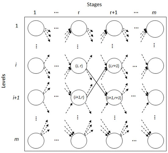
Figure 1. Illustration of the Multipartite Assignment Problem Graph (MAPG).

Each arc of our modeling graph (Figure 1) links nodes involving different levels at consecutive stages of the graph, with the tail node having the lower stage index. Hence, our modeling graph is both directed and multipartite. For convenience, given their centrality in our abstractions, we use the special notation “$⟨·⟩$” to represent the arcs of the graph. Specifically, a given arc $\left(\right(u,p),(v,p+1\left)\right)$ will be represented by “$⟨u,p,v⟩$” throughout this paper.

We assume that the Assignment Problem is balanced (i.e., that the two sets of objects being matched have the same cardinality). This causes no loss of generality, since fictitious stages (or levels) can be added to the graph as needed, with zero cost, to compensate for a deficit of stages (or levels). Moreover, no node or arc is excluded from our graph. This also does not reduce generality, since prohibited assignments in a given context can be handled in a linear optimization model by associating large (“Big-M”) costs to them.

We refer to our modeling graph as the “Multipartite Assignment Problem Graph (MAPG).” A formal statement of the graph and the path structures of it that underlie our modeling will be discussed below.

Notation 2 

(Graph Notations).

1. 

m: Number of assignments to be made.

2. 

${\mathcal{M}}_m$: Set of “full assignments”/bipartite matchings/assignment solutions of an m-Assignment Problem (m-AP).

3. 

${\mathcal{AP}}_m$: m-Assignment polytope (polytope with members of ${\mathcal{M}}_m$ as its extreme points).

4. 

$L:=\{1,\dots ,m\}$ (index set for the levels of the MAPG).

5. 

$S:=\{1,\dots ,m\}$ (index set for the stages of the MAPG).

6. 

$N:=\left\{(l,s)\in (L,S)\right\}$ (set of nodes of the MAPG).

7. 

$A:=\left\{⟨u,p,v⟩:((u,p),(v,p+1))\in N^2,(\forall p\in S\setminus \left\{m\right\}),(\forall (u,v)\in L^2(u\ne v))\right\}$ (set of arcs of the MAPG).

Definition 5 

(“Arc separation”). Let $p\ne q\in S$ and $⟨i_p,p,i_{p+1}⟩,⟨i_q,q,i_{q+1}⟩\in A.$ The “separation between $⟨i_p,p,i_{p+1}⟩$ and $⟨i_q,q,i_{q+1}⟩$” is the quantity $(\left|q-p\right|-1)$, and we denote it by “$SEP(⟨i_p,p,i_{p+1}⟩,$ $⟨i_q,q,i_{q+1}⟩)$”.

In other words, if $SEP(⟨i_p,p,i_{p+1}⟩,⟨i_q,q,i_{q+1}⟩)$ = δ (for some $\delta \in \mathbb{N}$), then either $(q=p+\delta +1)$ or $(p=q+\delta +1)$, and vice versa (i.e., if $(q=p+\delta +1)$ or $(p=q+\delta +1),$ then $SEP(⟨i_p,p,i_{p+1}⟩,⟨i_q,q,i_{q+1}⟩)$ = δ).

Definition 6 

(“Graph path”). Let $g,q\in S$ be such that $g+1<q<m.$ We define the following concepts and notations:

1. 

A “graph path (of the MAPG) (between arcs $⟨i_g,g,i_{g+1}⟩$ and $⟨i_q,q,i_{q+1}⟩$)” is an ordered tuple of arcs $B:=\left(⟨i_g,g,i_{g+1}⟩,⟨i_{g+1},g+1,i_{g+2}⟩,\dots ,⟨i_q,q,i_{q+1}⟩\right)$ with the following condition: $\{i_g,\dots ,i_{q+1}\}$ are pairwise-distinct.

2. 

The notation $gPath(B,⟨i_g,g,i_{g+1}⟩,⟨i_q,q,i_{q+1}⟩)$ indicates that “B is a graph path (of the MAPG) between $⟨i_g,g,i_{g+1}⟩$ and $⟨i_q,q,i_{q+1}⟩$.”

3. 

A “spanning graph path" is a graph path that starts at an arc at stage $g=1$ and ends at an arc at stage $q=m-1$. Hence, it has the form $B=\left(⟨i_1,1,i_2⟩,\dots ,⟨i_{m-1},m-1,i_m⟩\right),$ and we write it as “$sgPath(B;i_1,i_2,i_{m-1},i_m).$"

4. 

For pairwise-distinct $i_1,i_2,i_{m-1},i_m\in L,$ let $V:=$ $L\setminus \{i_1,i_2,i_{m-1},i_m\}$ be expressed in terms of its natural increasing order as $V=\{v_3,\dots ,v_{m-2}\},$ where $v_3<v_4<\dots <v_{m-2}.$ For $\sigma \in Sym(V)$, define spanning graph path $G_{i_1,i_2,i_{m-1},i_m}^{\sigma }:$

$$\begin{array}{cc}\hfill G_{i_1,i_2,i_{m-1},i_m}^{\sigma }:=& \left(⟨i_1,1,i_2⟩,⟨i_2,2,\sigma (v_3)⟩,\dots ,⟨\sigma (v_k),k,\sigma (v_{k+1})⟩,\dots ,\right.\hfill \\ \hfill & \left.⟨\sigma (v_{m-2}),m-2,i_{m-1}⟩,⟨i_{m-1},m-1,i_m⟩\right).\hfill \end{array}$$

5. 

The set of all the spanning graph paths of MAPG is denoted as ${\mathsf{\Gamma }}_m$ and explicitly expressed by the following:

$$\begin{array}{cc}\hfill {\mathsf{\Gamma }}_m:=& \{G_{i_1,i_2,i_{m-1},i_m}^{\sigma }:i_1,i_2,i_{m-1},i_m\in L\mathit{are}\mathit{pairwise-distinct},\hfill \\ \hfill & \sigma \in Sym(L\setminus \{i_1,i_2,i_{m-1},i_m\})\}.\hfill \end{array}$$

The significance of these graph paths resides in their one-to-one correspondence with assignment solutions, as shown in the following theorem.

Theorem 3 

(Graph Paths ⟷ AP Solutions). The mapping $f_1:{\mathsf{\Gamma }}_m\to {\mathcal{M}}_m$ is bijective.

Proof. 

First, the number of quadruplets $(i_1,i_2,i_{m-1},i_m)\in L^4$ with pairwise-distinct members is $(m$ · $(m-1)$ · $(m-2)$ · $(m-3))$. The number of permutations of the members of the remaining $L\setminus \{i_1,i_2,i_{m-1},i_m\}$ set of levels is $(m-4)!$. Hence, $|{\mathsf{\Gamma }}_m|$=m · $(m-1)$ · $(m-2)$ · $(m-3)$ · $(m-4)!$ = $m!$.

Second, it is a well-known result that the number of full assignments of an m-AP is $|{\mathcal{M}}_m| = m!$.

Finally, we have $|{\mathsf{\Gamma }}_m|$ = $|{\mathcal{M}}_m|$ = $m!,$ and the theorem follows directly. □

Our modeling consists of developing constraints whose feasible set decomposes by subsets, each of which corresponds to exactly one of the spanning graph paths of the MAPG. Since this task involves “picking out” particular arcs in a graph, a well-suited framework for it in Mathematical Programming is that of network flow modeling.

4. $\mathsf{\Theta }$(m)⁹ Ternary Network Flow Model of the AP Polytope

The framework of our LP modeling follows that of a minimum-cost network flow problem (see [4], pp. 453–512; among others). The idea is to develop an abstraction of the spanning graph paths of the MAPG discussed above. This requires complex flow variables, resulting in a higher-dimensional linear program (LP) model of the Assignment Problem (AP; [4], pp. 535–550; [5]) polytope. Our modeling variables involve triplets of arcs from the underlying graph (i.e., the MAPG). Hence, we refer to our proposed model as a “ternary model” (see [18,19]).

Our Kirchhoff Equations (KEs)/“flow-balance”/“mass-conservation” constraints are “complex” because they are parametrized by the arcs that index the specific variables involved in them respectively. We refer to these as “Generalized Kirchhoff Equations (GKEs).” They induce a structure of differently labeled, super-imposed, but non-separable/non-independent layers of flow through the MAPG. By being layered, these flows are akin to “commodity flows” in a multicommodity flow context; however, their nonseparability distinguishes them from “commodity flows”.

Other constraints of our model enforcing flow-balance/mass-conservation requirements across the stages of the MAPG pertain to “boundary flow conditions,” as every pair of arcs in the modeling may be viewed as a potential source, and every node as a potential destination. We refer to these constraints as the “Flow Consistency Constraints.” A third class of constraints (which we call “Visit Requirements Constraints”) serves to enforce flow-balance/mass-conservation conditions across the levels of the flow graph, MAPG. Finally, there is a constraint that initiates a unit flow at the first stage of the flow graph, and there is a class of constraints that serve to preclude implicitly zero (logically zero) variables from being considered in the Assignment decision making. These are necessary to ensure flow connectedness and prevent flow from “re-visiting” a level (i.e., to avoid “self-loops” or cycles being allowed within individual variables).

4.1. Model Variables

Notation 3 

(Modeling variables). For $(⟨i_g,g,j_g⟩,⟨i_p,p,j_p⟩,⟨i_q,q,j_q⟩)\in A^3$ pairwise-distinct, we define the following:

1. 

$x_{⟨i_g,g,j_g⟩⟨i_p,p,j_p⟩⟨i_q,q,j_q⟩}$: Variable indicating the simultaneous assignments of levels $i_g,$$j_g,$$i_p,$$j_p,$$i_q,$ and $j_q$ to stages g, $g+1$, p, $p+1,$ q, and $q+1$, respectively.

2. 

$\overline{x}\left(⟨i_g,g,j_g⟩,⟨i_p,p,j_p⟩,⟨i_q,q,j_q⟩\right)$: Function that returns the x-variable with the arc indices arranged in increasing order of the stage indices. Specifically,

$\overline{x}\left(⟨i_g,g,j_g⟩,⟨i_p,p,j_p⟩,⟨i_q,q,j_q⟩\right):=\left\{\begin{array}{c}{x}_{⟨i_g,g,j_g⟩⟨i_p,p,j_p⟩⟨i_q,q,j_q⟩}\mathit{if}g<p<q;\hfill \\ \\ x_{⟨i_g,g,j_g⟩⟨i_q,q,j_q⟩⟨i_p,p,j_p⟩}\mathit{if}g<q<p;\hfill \\ \\ x_{⟨i_p,p,j_p⟩⟨i_g,g,j_g⟩⟨i_q,q,j_q⟩}\mathit{if}p<g<q;\hfill \\ \\ x_{⟨i_p,p,j_p⟩⟨i_q,q,j_q⟩⟨i_g,g,j_g⟩}\mathit{if}p<q<g;\hfill \\ \\ x_{⟨i_q,q,j_q⟩⟨i_g,g,j_g⟩⟨i_p,p,j_p⟩}\mathit{if}q<g<p;\hfill \\ \\ x_{⟨i_q,q,j_q⟩⟨i_p,p,j_p⟩⟨i_g,g,j_g⟩}\mathit{if}q<p<g;\hfill \\ \\ 0\mathit{otherwise}.\hfill \end{array}\right..$

Remark 1. 

1. 

$\overline{x}(·)$ is used for the purpose of simplifying the exposition only. The domain of x is the region of ${\mathbb{R}}^{m^9}$ specified in Section 4.2 of this paper.

2. 

We interpret variable $x_{⟨i_g,g,j_g⟩⟨i_p,p,j_p⟩⟨i_q,q,j_q⟩}$ as the amount of flow that traverses all three of the arcs $⟨i_g,g,j_g⟩$, $⟨i_p,p,j_p⟩$, and $⟨i_q,q,j_q⟩$ jointly, and we will refer to it as the “joint-flow" of the three arcs whenever that is convenient.

3. 

We also say that two given arcs have “joint-flow” if they jointly index a positive variable.

Definition 7 

(“Support graph (of x)”). Let $x\in {\mathbb{R}}_{\ge 0}^{m^9}$ be specified as in Notation 3. The “support graph of x” is ${\overline{H}}_x=({\overline{A}}_x,{\overline{N}}_x)$ with ${\overline{A}}_x:=\{⟨i_g,g,j_g⟩\in A:\left(\right(\exists ⟨i_p,p,j_p⟩,$ $⟨i_q,q,j_q⟩\in A)$ $[\overline{x}(⟨i_g,g,j_g⟩,$ $⟨i_p,p,j_p⟩,$ $⟨i_q,q,j_q⟩)>0]\left)\right\},$ and ${\overline{N}}_x$ $:=$ $\left\{\right(u,q)\in N:(\exists v\in L)$ $[⟨v,q-1,u⟩\in {\overline{A}}_x\in ⟨u,q,v⟩\in {\overline{A}}_x\left]\right\}.$

Remark 2. 

Let $x\in {\mathbb{R}}_{\ge 0}^{m^9}$ be as specified in Notation 3. We have the following:

1. 

$supp\left(x\right)=\{(\mathbf{a},\mathbf{b},\mathbf{c})\in A^3:x_{\mathbf{a},\mathbf{b},\mathbf{c}}>0\}.$

2. 

The support graph of x, ${\overline{H}}_x$, is the subgraph of the MAPG comprising the arcs that index the positive components of x and the nodes upon which those arcs are incident.

3. 

Let P be a collection of distinct arc triples (e.g., P may be specified as a subset $P\subseteq A^3$ or as a tuple of elements of $A^3,$ $P=(({\mathbf{a}}_{\mathbf{1}},{\mathbf{b}}_{\mathbf{1}},{\mathbf{c}}_{\mathbf{1}}),\dots ,({\mathbf{a}}_{\mathbf{k}},{\mathbf{b}}_{\mathbf{k}},{\mathbf{c}}_{\mathbf{k}})),$ with no repeated entries). The indicator vector of P relative to x, $I_x\left(P\right)\in {\{0,1\}}^{A^3}$, is specified by the following (see Definition 4):

$$\begin{array}{cc}\hfill & {\left(I_x\left(P\right)\right)}_{(\mathbf{a},\mathbf{b},\mathbf{c})}=\left\{\begin{array}{c}1\mathit{if}(\mathbf{a},\mathbf{b},\mathbf{c})\in (P\cap supp(x\left)\right),\hfill \\ \\ 0\mathit{otherwise},\hfill \end{array}\right.\hfill \\ \hfill & \mathit{for}\mathit{all}\mathbf{a},\mathbf{b},\mathbf{c}\in A.\hfill \end{array}$$

As shown in Remark 2.1 above, for each $x\in {\mathbb{R}}_{\ge 0}^{m^9},$ $supp\left(x\right)$ is a ternary relation over the set of arcs. We give a formalization of this through the following definition and show some immediate, foundational results.

Definition 8 

(“$Support$ $relation-in-x$ $\left({\mathbb{S}}_x\right)$”). Let $x\in {\mathbb{R}}_{\ge 0}^{m^9}$ be as specified in Notation 3. The support relation, ${\mathbb{S}}_x\subseteq A^3,$ is a ternary relation we define by

$$({\mathbf{a}}_{\mathbf{g}},{\mathbf{a}}_{\mathbf{p}},{\mathbf{a}}_{\mathbf{q}})\in {\mathbb{S}}_x\mathit{if}\mathit{and}\mathit{only}\mathit{if}\overline{x}({\mathbf{a}}_{\mathbf{g}},{\mathbf{a}}_{\mathbf{p}},{\mathbf{a}}_{\mathbf{q}})>0,$$

for all pairwise-distinct $g,$ $p,$ $q\in S,$ for all ${\mathbf{a}}_{\mathbf{g}}=⟨i_g,g,j_g⟩\in A,$ ${\mathbf{a}}_{\mathbf{p}}=⟨i_p,p,j_p⟩\in A$, and ${\mathbf{a}}_{\mathbf{q}}=⟨i_q,q,j_q⟩\in A$.

Some good/classic references on relations are [18,19,21].

Theorem 4 

(Symmetry of ${\mathbb{S}}_{\mathit{x}}$).  For every $x\in {\mathbb{R}}_{\ge 0}^{m^9}$ specified in Notation 3,${\mathbb{S}}_x$ (see Definition 8) is symmetric.

Proof. 

Let $x\in {\mathbb{R}}_{\ge 0}^{m^9}.$ We will show that ${\mathbb{S}}_x$ is invariant under all permutations of its arguments, which is the definition of symmetry.

Let $\mathbf{a},\mathbf{b},\mathbf{c}\in A$ be pairwise-distinct. Let $\pi$ be any permutation of three elements.

By definitional notations (specifically, Notation 3.2), the function $\overline{x}(·)$ is invariant under all the permutations of its arguments by $\pi$.

Suppose $(\mathbf{a},\mathbf{b},\mathbf{c})\in {\mathbb{S}}_x$. Then, $\overline{x}(\mathbf{a},\mathbf{b},\mathbf{c})>0.$ The invariance of $\overline{x}(·)$ implies $\overline{x}\left(\pi (\mathbf{a},\mathbf{b},\mathbf{c})\right)$ = $\overline{x}(\mathbf{a},\mathbf{b},\mathbf{c})$ > 0. Therefore, $\pi (\mathbf{a},\mathbf{b},\mathbf{c})\in {\mathbb{S}}_x.$

Conversely, suppose $\pi (\mathbf{a},\mathbf{b},\mathbf{c})\in$ ${\mathbb{S}}_x.$ Then, $\overline{x}\left(\pi (\mathbf{a},\mathbf{b},\mathbf{c})\right)$ $>0.$ Applying the reverse permutation ${\pi }^{-1}$ and using the invariance of $\overline{x}(·),$ we have $\overline{x}\left({\pi }^{-1}\left(\pi (\mathbf{a},\mathbf{b},\mathbf{c})\right)\right)$ = $\overline{x}(\mathbf{a},\mathbf{b},\mathbf{c})$ > $0.$ Hence, $(\mathbf{a},\mathbf{b},\mathbf{c})$∈ ${\mathbb{S}}_x.$

Therefore, ${\mathbb{S}}_x$ is symmetric for every $x\in {\mathbb{R}}_{\ge 0}^{m^9}$. □

Definition 9 

(“Support-clique of x” (“${\mathbb{S}}_x$-clique”)). Let $x\in {\mathbb{R}}_{\ge 0}^{m^9}$ be as specified in Notation 3. A collection, P, of 3 or more pairwise-distinct arcs of A is a “support-clique (of x)” (denoted by “${\mathbb{S}}_x$-$clique$”) if and only if for all pairwise-distinct $\mathbf{a}$, $\mathbf{b}$, $\mathbf{c}\in P,$ $(\mathbf{a},\mathbf{b},\mathbf{c})\in {\mathbb{S}}_x.$

Remark 3. 

For clarity, a ${\mathbb{S}}_x$-$clique$ may be referred to as a “k-${\mathbb{S}}_x$-$clique$” when k is the number of members (i.e., the set cardinality or the tuple length) of the collection.

4.2. Model Constraints

As discussed above, our proposed LP is essentially a minimum-cost network flow model, but it relies on a more complex notion of “flow.” One unit of this “complex flow” is initiated at the first stage of our flow graph, with different “labels” assigned to it over the first four stages of the MAPG by an “Initial Flow” constraint. These “labeled flows” are then propagated throughout the MAPG in a connected manner, acquiring additional labels progressively through our parametrized Kirchhoff Equations (i.e., the GKEs). Hence, our proposed formulation captures the essence of a shortest-path model. Additionally, the model includes a stipulation (the “Visit Requirements” constraints) that flow “visit”/propagate to each level of the graph equally. With this “cross-level” balancing/conservation stipulation, the model also captures the essence of an Assignment Problem formulation (since the underlying graph is basically a graphical representation of an Assignment tableau and the GKEs also constrain flow to “visit” each stage equally).

4.2.1. Statement of the Constraints

We start with the class of constraints which set some variables to zero based on logical conditions.

• “Implicit-Zeros (IZ)” constraints.

  $$\begin{array}{cc}\hfill & x_{⟨i_g,g,j_g⟩⟨i_p,p,j_p⟩⟨i_q,q,j_q⟩}=0\mathrm{if}\hfill \\ \hfill & \left(i\right)\mathbf{not}(g<p<q);\mathrm{or}\hfill \\ \hfill & \left(ii\right)(p>g+1)\wedge (q>p+1)\wedge (i_g,j_g,i_p,j_p,i_q,j_q\mathbf{not}\mathrm{pairwise-distinct});\mathrm{or}\hfill \\ \hfill & \left(iii\right)(p=g+1)\wedge (q>p+1)\wedge \left(\mathbf{not}(i_p=j_g)\vee \right.\hfill \\ \hfill & (i_g,j_g,j_p,i_q,j_q\mathbf{not}\mathrm{pairwise}\mathrm{distinct}));or\hfill \\ \hfill & \left(iv\right)(p>g+1)\wedge (q=p+1)\wedge (\mathbf{not}(i_q=j_p)\vee \hfill \\ \hfill & (i_g,j_g,i_p,j_p,j_q\mathbf{not}\mathrm{pairwise-distinct}));\mathrm{or}\hfill \\ \hfill & \left(v\right)(p=g+1)\wedge (q=p+1)\wedge (\mathbf{not}(i_p=j_g)\vee \mathbf{not}(i_q=j_p)\vee \hfill \\ \hfill & (i_g,j_g,j_p,j_q\mathbf{not}\mathrm{pairwise-distinct})).\hfill \end{array}$$

  (10)
• Explicit constraints that are vacuous due to the Implicit-Zeros constraints (10) need to be excluded from consideration by properly scoping the quantifiers used. For this purpose, let $(g,q)\in S$ with $g<q<m.$ In stating the remainder constraints, we will use the following:

  –

  Stages to be excluded from consideration:

  $$E_{g,q}:=\{p\in S:p\ne g,g+1,q,q+1\}$$

  –

  Levels to be fixed for connectedness:

  $$\begin{array}{cc}\hfill F_{g,q}:=& \{(a,b,c,d)\in L^4:((a,b,c,d\mathrm{are}\mathrm{pairwise-distinct},\mathrm{if}g+1<q)\wedge \hfill \\ \hfill & (a,b,d\mathrm{are}\mathrm{pairwise-distinct}\mathrm{with}c=b,\mathrm{if}g+1=q)\left)\right\}.\hfill \end{array}$$

  The remaining classes of constraints will now be stated.

• Initial Flow (IF) constraints.

  $$\sum _{i_1=1}^m\sum _{i_2=1}^m\sum _{i_3=1}^m\sum _{i_4=1}^m{x}_{⟨i_1,1,i_2⟩⟨i_2,2,i_3⟩⟨i_3,3,i_4⟩}=1.$$

  (11)
• Generalized Kirchhoff Equations (GKEs)

  $$\begin{array}{cc}\hfill & \sum _{k=1}^m\overline{x}\left(⟨i_g,g,j_g⟩,⟨i_q,q,j_q⟩,⟨i_p,p,k⟩\right)-\hfill \\ \hfill & \sum _{k=1}^m\overline{x}\left(⟨i_g,g,j_g⟩,⟨i_q,q,j_q⟩,⟨k,p-1,i_p⟩\right)=0;\forall g,q\in S\mathrm{with}g<q<m,\hfill \\ \hfill & \forall p\in E_{g,q}\setminus \{1,m\},\forall (i_g,j_g,i_q,j_q)\in F_{g,q},\forall i_p\in L\mathrm{with}{i}_p\ne i_g,j_g,i_q,j_q.\hfill \end{array}$$

  (12)
• Flow Consistency (FC) constraints.
  Define ${\Delta }_{gq}^S\left(p\right):=\{min\delta \in \{1,\dots ,m-p\}:(p+\delta )\notin \{g,q\}\}.$

  $$\begin{array}{cc}\hfill & \sum _{k=1}^m\sum _{t=1}^m\overline{x}\left(⟨i_g,g,j_g⟩,⟨i_q,q,j_q⟩,⟨k,p,t⟩\right)-\hfill \\ \hfill & \sum _{k=1}^m\sum _{t=1}^m\overline{x}\left(⟨i_g,g,j_g⟩,⟨i_q,q,j_q⟩,⟨k,p+{\Delta }_{gq}^S\left(p\right),t⟩\right)=0;\hfill \\ \hfill & \forall g,q\in S\mathrm{with}g<q<m,\forall p\in E_{g,q},\forall (i_g,j_g,i_q,j_q)\in F_{g,q}.\hfill \end{array}$$

  (13)
• Visit Requirements (VR) constraints.
  Define ${\Delta }_{i_g,j_g,i_q,j_q}^L\left(u\right):=\{min\delta \in \{1,\dots ,m-u\}:(u+\delta )\notin \{i_g,j_g,i_q,j_q\}\}.$
  Let ${\mathcal{U}}_{i_g,j_g,i_q,j_q}$ = $\{u\in L:u\le m-{\Delta }_{i_g,j_g,i_q,j_q}^L\left(u\right),u\ne i_g,j_g,i_q,j_q\}.$

  $$\begin{array}{cc}\hfill & \sum _{r=1}^{g-1}\sum _{k=1;}^m\overline{x}\left(⟨i_g,g,j_g⟩,⟨i_q,q,j_q⟩,⟨u,r,k⟩\right)+\hfill \\ \hfill & \sum _{r=g+2;r\ne q,q+1}^m\sum _{k=1}^m\overline{x}\left(⟨i_g,g,j_g⟩,⟨i_q,q,j_q⟩,⟨k,r-1,u⟩\right)-\hfill \\ \hfill & \sum _{r=1}^{g-1}\sum _{k=1}^m\overline{x}\left(⟨i_g,g,j_g⟩,⟨i_q,q,j_q⟩,⟨u+{\Delta }_{i_g,j_g,i_q,j_q}^L\left(u\right),r,k⟩\right)-\hfill \\ \hfill & \sum _{r=g+2;r\ne q,q+1}^m\sum _{k=1}^m\overline{x}\left(⟨i_g,g,j_g⟩,⟨i_q,q,j_q⟩,⟨k,r-1,u+{\Delta }_{i_g,j_g,i_q,j_q}^L\left(u\right)⟩\right)=0;\hfill \\ \hfill & \forall g,q\in S\mathrm{with}g<q<m,\forall (i_g,j_g,i_q,j_q)\in F_{g.q},\forall u\in {\mathcal{U}}_{i_g,j_g,i_q,j_q}.\hfill \end{array}$$

  (14)
• Nonnegativity (NN) constraints.

  $$x_{⟨i_g,g,j_g⟩⟨i_p,p,j_p⟩⟨i_q,q,j_q⟩}\ge 0;\forall i_g,g,j_g,i_p,p,j_p,i_q,q,j_q\in \{1,\dots ,m\}.$$

  (15)

The IZ constraints (10) ensure that joint-flow is not broken and does not “re-visit” at the level of the individual x-variables. One unit of flow is initiated and “labeled” with arcs at the first four stages of our flow graph (MAPG) by constraint (11). This flow is propagated through the graph of stages by constraints (12), which are parametrized forms of the standard “mass/joint-flow balance” equations, known as Kirchhoff Equations. We refer to these constraints as the Generalized Kirchhoff Equations (GKEs). They stipulate that the joint-flow of two given arcs entering a node must be equal to the joint-flow of the two arcs leaving the node. In constraints (13), $(p$ + ${\Delta }_{gq}^S\left(p\right))$ is the index of the first stage after p, which is distinct from stages g and q. Hence, these constraints stipulate that the joint-flow traversing any stage of the MAPG must be the same across all the stages. These constraints are non-redundant only at boundary joint-flow conditions and ensure that the joint-flow of two given nodes is balanced across either of those nodes. In Visit Requirements constraints (14), $(u$ + ${\Delta }_{i_g,j_g,i_q,j_q}^L\left(u\right))$ is the index of the first level after u that is distinct from levels $i_g,$ $j_g,$ $i_q,$ and $j_q$. Hence, these constraints stipulate that the joint-flow of two given arcs propagating to a given level of the MAPG is the same for all MAPG levels, thereby ensuring the “mass/joint-flow balance” conditions across the levels. Finally, Nonnegativity constraints (15) are the usual ones on the modeling variables.

Notation 4 

(Polytope $Q;$ Set $Q_I$).

1. 

$Q:=\{x\in {\mathbb{R}}^{m^9}:x$ satisfies (10)–(15)} (“the LP polytope").

2. 

$Q_I:=\{x\in Q:x$ is integral} (set of the integral points of the LP polytope).

4.2.2. Valid Constraints

Lemma 1 

(Valid Constraints for Q).  The following constraints are valid for the LP polytope, Q:

$$\begin{array}{cc}\hfill & \sum _{k=1}^m\sum _{t=1}^m{x}_{⟨i_g,g,j_g⟩⟨k,p,t⟩⟨i_q,q,j_q⟩}-\sum _{k=1}^m\sum _{t=1}^m{x}_{⟨i_g,g,j_g⟩⟨k,r,t⟩⟨i_q,q,j_q⟩}=0;\hfill \\ \hfill & \forall g,p,q,r\in S\mathit{with}(q<m\wedge g<p<q\wedge g<r<q),\forall (i_g,j_g,i_q,j_q)\in F_{g,q}.\hfill \end{array}$$

(16)

$$\begin{array}{cc}\hfill & \sum _{k=1}^m{x}_{⟨i_g,g,j_g⟩⟨j_g,g+1,k⟩⟨i_q,q,j_q⟩}-\sum _{k=1}^m{x}_{⟨i_g,g,j_g⟩⟨k,q-1,i_q⟩⟨i_q,q,j_q⟩}=0;\hfill \\ \hfill & \forall g,q\in S\mathit{with}g+1<q<m,\forall (i_g,j_g,i_q,j_q)\in F_{g,q}.\hfill \end{array}$$

(17)

$$\begin{array}{cc}\hfill & \sum _{i_g=1}^m\sum _{j_g=1}^m\sum _{i_p=1}^m\sum _{j_p=1}^m\sum _{i_q=1}^m\sum _{j_q=1}^m{x}_{⟨i_g,g,j_g⟩⟨i_p,p,j_p⟩⟨i_q,q,j_q⟩}-\hfill \\ \hfill & \sum _{i_h=1}^m\sum _{j_h=1}^m\sum _{i_r=1}^m\sum _{j_r=1}^m\sum _{i_s=1}^m\sum _{j_s=1}^m{x}_{⟨i_h,h,j_h⟩⟨i_r,r,j_r⟩⟨i_s,s,j_s⟩}=0;\hfill \\ \hfill & \forall g,p,q,h,r,s\in S\mathit{with}(g<p<q<m)\wedge (h<r<s<m).\hfill \end{array}$$

(18)

$$\begin{array}{cc}\hfill & \sum _{i_g=1}^m\sum _{j_g=1}^m\sum _{i_p=1}^m\sum _{j_p=1}^m\sum _{i_q=1}^m\sum _{j_q=1}^m{x}_{⟨i_g,g,j_g⟩⟨i_p,p,j_p⟩⟨i_q,q,j_q⟩}=1;\hfill \\ \hfill & \forall g,p,q\in S\mathit{with}g<p<q<m.\hfill \end{array}$$

(19)

Proof. 

1.

Flow-Consistency constraints (13) stipulate that the total joint flow of two given arcs, $⟨i_g,g,j_g⟩$ and $⟨i_q,q,j_q⟩$, which propagate through/traverses a stage of the MAPG, is the same for all MAPG stages. Hence, these constraints (constraints (13)) can be equivalently expressed (although less parsimoniously) as

$$\begin{array}{cc}\hfill & \sum _{k=1}^m\sum _{t=1}^m\overline{x}\left(⟨i_g,g,j_g⟩,⟨i_q,q,j_q⟩,⟨k,p,t⟩\right)-\hfill \\ \hfill & \sum _{k=1}^m\sum _{t=1}^m\overline{x}(⟨i_g,g,j_g⟩,⟨i_q,q,j_q⟩,⟨k,r,t⟩)=0;\hfill \\ \hfill & \forall g,q,p,r\in S\mathrm{with}(g<q<m\wedge p,r\notin \{g,q\left\}\right)\wedge p\ne r,\hfill \\ \hfill & \forall (i_g,j_g,i_q,j_q)\in F_{g,q}.\hfill \end{array}$$

(20)

Constraints (16) are a special case of constraints (20), where “p” and “r” are, respectively, strictly between “g” and “q”.

2.

Constraints (17) are obtained by using Implicit-Zeros constraints (10) to exclude implicitly zero variables from constraints (16) for the special case of $p=g+1$ and $r=q-1$.

3.

Summing over all the levels involved in (20) and then using the associativity of addition to recursively re-group terms according to pairs of stages gives the following:

$(\forall g,p,q,h,r,s\in S\setminus \{m\}$ pairwise-distinct),

${\displaystyle \sum _{i_g=1}^m}{\displaystyle \sum _{j_g=1}^m}{\displaystyle \sum _{i_q=1}^m}{\displaystyle \sum _{j_q=1}^m}\left({\displaystyle \sum _{i_p=1}^m}{\displaystyle \sum _{j_p=1}^m}\overline{x}(⟨i_g,g,j_g⟩,⟨i_q,q,j_q⟩,⟨i_p,p,j_p⟩)\right)$

$={\displaystyle \sum _{i_g=1}^m}{\displaystyle \sum _{j_g=1}^m}{\displaystyle \sum _{i_q=1}^m}{\displaystyle \sum _{j_q=1}^m}\left({\displaystyle \sum _{i_h=1}^m}{\displaystyle \sum _{j_h=1}^m}\overline{x}(⟨i_g,g,j_g⟩,⟨i_q,q,j_q⟩,⟨i_h,h,j_h⟩)\right)$(Using (20))

$={\displaystyle \sum _{i_q=1}^m}{\displaystyle \sum _{j_q=1}^m}{\displaystyle \sum _{i_h=1}^m}{\displaystyle \sum _{j_h=1}^m}\left({\displaystyle \sum _{i_g=1}^m}{\displaystyle \sum _{j_g=1}^m}\overline{x}(⟨i_q,q,j_q⟩,⟨i_h,h,j_h⟩,⟨i_g,g,j_g⟩)\right)$(Re-grouping)

$={\displaystyle \sum _{i_q=1}^m}{\displaystyle \sum _{j_q=1}^m}{\displaystyle \sum _{i_h=1}^m}{\displaystyle \sum _{j_h=1}^m}\left({\displaystyle \sum _{i_r=1}^m}{\displaystyle \sum _{j_r=1}^m}\overline{x}(⟨i_q,q,j_q⟩,⟨i_h,h,j_h⟩,⟨i_r,r,j_r⟩)\right)$(Using (20))

$={\displaystyle \sum _{i_h=1}^m}{\displaystyle \sum _{j_h=1}^m}{\displaystyle \sum _{i_r=1}^m}{\displaystyle \sum _{j_r=1}^m}\left({\displaystyle \sum _{i_q=1}^m}{\displaystyle \sum _{j_q=1}^m}\overline{x}(⟨i_h,h,j_h⟩,⟨i_r,r,j_r⟩,⟨i_q,q,j_q⟩)\right)$(Re-grouping)

$={\displaystyle \sum _{i_h=1}^m}{\displaystyle \sum _{j_h=1}^m}{\displaystyle \sum _{i_r=1}^m}{\displaystyle \sum _{j_r=1}^m}\left({\displaystyle \sum _{i_s=1}^m}{\displaystyle \sum _{j_s=1}^m}\overline{x}(⟨i_h,h,j_h⟩,⟨i_r,r,j_r⟩,⟨i_s,s,j_s⟩)\right)$(Using (20)).

Constraints (18) are a special case of the last item in the sequence of the equalities above, where $(g<p<q<m)$ and $(h<r<s<m)$.

4.

From Implicit-Zeros constraints (10), we have

$$\begin{array}{cc}\hfill & (\forall g\in S\mathrm{with}g<m-2)(\forall i_g,j_g,i_{g+1},j_{g+1},i_{g+2},j_{g+2}\in L)\hfill \\ \hfill & [((i_{g+1}\ne j_g)\vee (i_{g+2}\ne j_{g+1})\vee \neg (j_{g+2}\ne i_g,j_g,i_{g+1},j_{g+1},i_{g+2}))\Rightarrow \hfill \\ \hfill & x_{⟨i_g,g,j_g⟩⟨i_{g+1},g+1,j_{g+1}⟩⟨i_{g+2},g+2,j_{g+2}⟩}=0].\hfill \end{array}$$

(21)

Using (21), constraints (11) can be re-written in a form that includes implicitly zero variables:

$$\sum _{i_1=1}^m\sum _{j_1=1}^m\sum _{i_2=1}^m\sum _{j_2=1}^m\sum _{i_3=1}^m\sum _{j_3=1}^m{x}_{⟨i_1,1,j_1⟩⟨i_2,2,j_2⟩⟨i_3,3,j_3⟩}=1.$$

(22)

Constraints (19) follow directly from the combination of (18) and (22).

□

Corollary 1 

($\mathbf{0}\le \mathit{x}\le \mathbf{1}$). The results below follow directly:

1. 

$Q\subseteq {[0,1]}^{m^9}$ (from valid constraints (19) and nonnegativity constraints (15)).

2. 

$Q_I\subseteq {\{0,1\}}^{m^9}$ (from $\left(1\right)$ above).

3. 

$Q_I\subseteq ext\left(Q\right)$ (from (1)–(2) above and IPE Theorem 1).

4.3. Model Size

In this section, we provide a formal proof of the polynomial size of our proposed model, Q.

Theorem 5 

(Model size). Q is polynomial-sized, with:

1. 

$\mathsf{\Theta }\left(m^9\right)$ variables;

2. 

$\mathsf{\Theta }\left(m^8\right)$ constraints.

Proof. 

The variables of Q are of the form $x_{⟨i_g,g,j_g⟩⟨i_p,p,j_p⟩⟨i_q,q,j_q⟩}$, where $1\le g<p<q\le m-1$ and $i_g,j_g,i_p,j_p,i_q,j_q\in \{1,\dots ,m\}.$ Implicit-Zeros constraints (10) exclude some of these variables by restricting them to 0. These excluded variables must be correctly accounted for in the process of assessing the numbers of variables and constraints.

1.

Number of variables.

We will consider the different cases based on the restrictions of constraints (10).

Case 1 (Fully consecutive arcs): $p=g+1$; $q=g+2$.

In this case, g ranges from 1 to $m-3$, giving $(m-3)$ choices for $(g,p,q)$. Constraints (10) require $i_p=j_g;$ $i_q=j_p;$ and $i_g,j_g,j_p,j_q$ distinct. The number of level assignments is as follows:

$${\displaystyle \frac{m!}{(m-4)!}}=m(m-1)(m-2)(m-3).$$

Hence, the number of variables representing “fully consecutive” arcs is

$$m(m-1)(m-2){(m-3)}^2$$

(23)

Case 2 (First two arcs consecutive; third arc separated): $p=g+1$; $q\ge g+3$.

Then, g ranges from 1 to $m-4$ and q ranges from $g+3$ to $m-1$. Hence, for each choice of g, there are $(m-1-(g+3)+1)=$ $(m-3-g)$ choices for q. The total number of choices for the $(g,p,q)$ triplet is

$${\displaystyle \sum _{k=1}^{m-4}}(m-3-k)={\displaystyle \sum _{k=1}^{m-4}}(m-3)-{\displaystyle \sum _{k=1}^{m-4}}k={\displaystyle \frac{(m-4)(m-3)}{2}}$$

Therefore, the number of choices for $(g,p,q)$ is ${(m-4)}^2(m-3)/2.$ Constraints (10) require $i_p=j_g;$ and $i_g,j_g,j_p,i_q,j_q$ distinct. The number of level assignments is as follows:

$${\displaystyle \frac{m!}{(m-5)!}}=m(m-1)(m-2)(m-3)(m-4)$$

Therefore, the number of variables representing “third-arc separated” case is as follows:

$$m(m-1)(m-2){(m-3)}^2{(m-4)}^2/2$$

(24)

Case 3 (First arc separated; last two arcs consecutive): $p\ge g+2$; $q=p+1$.

By symmetry, the number of variables in this case is given by (24).

Case 4 (All three arcs separated): $p\ge g+2$; $q\ge p+2$.

Then, g ranges from 1 to $m-5$, p ranges from $g+2$ to $m-3$, and q ranges from $p+2$ to $m-1$.

The number of possible choices for q for each p is $(m-1)-(p+2)+1=(m-p-2).$ Summing $(m-p-2)$ over p going from $(g+2)$ to $(m-3)$ gives ${\displaystyle \frac{(m-g-3)(m-g-4)}{2}}$ possible triplets $(g,p,q)$ for each choice of g. Let $k=m-g-4$. Then, when $g=1$, $k=m-5$. When $g=m-5$, $k=1.$ Hence, the number of (all) possible $(g,p,q)$ choices is

$${\displaystyle \frac{1}{2}}{\displaystyle \sum _{k=1}^{m-5}}\left(k\right)(k+1)={\displaystyle \frac{(m-5)(m-4)(m-3)}{6}}$$

Constraints (10) require $i_g,j_g,i_p,j_p,i_q,j_q$ to be distinct. Therefore, the number of level assignments is

$${\displaystyle \frac{m!}{(m-6)!}}=m(m-1)(m-2)(m-3)(m-4)(m-5).$$

Hence, the total number of variables with “all three arcs separated“ is as follows:

$${\displaystyle \frac{m(m-1)(m-2){(m-3)}^2{(m-4)}^2{(m-5)}^2}{6}}$$

(25)

Conclusion. The total number of variables, $V\left(m\right)$, is the polynomial function of m, which is the sum of expressions (23), (25), and expression (24) twice. The leading term of $V\left(m\right)$ is ${\displaystyle \frac{1}{6}}{m}^9.$ Therefore, the number of variables of Q is $\mathsf{\Theta }\left(m^9\right)$ (see [23], pp. 1–4). The first statement of the theorem has been proven.

2.

Number of constraints.

Define the following:

-

$\mathbb{I}[$“*”$]=\left\{\begin{array}{c}1\mathrm{if}“*”\mathrm{is}\mathrm{TRUE};\hfill \\ \\ 0\mathrm{otherwise}.\hfill \end{array}\right.$

- $P_3:={\displaystyle \frac{m!}{(m-3)!}}=m(m-1)(m-2).$

(a)

Initial Flow (IF) Constraints.

The number of IF constraints is 1.

(b)

Generalized Kirchhoff Equation (GKE) Constraints.

• Case 1:  $\mathbf{q}=\mathbf{g}+\mathbf{1}.$
  - $(g,q):(m-2)$ choices.
  - $F_{g,q}:P_3$ choices;
  - $i_p:(m-3)$ choices.
  - $p:(m-3)-\mathbb{I}[1\in E_{g,q}]-\mathbb{I}[m\in E_{g,q}]$ choices.
    $=\left\{\begin{array}{c}(m-4)\mathrm{if}(g=1)\vee (g=m-2);\hfill \\ (m-5)\mathrm{if}2\le g\le (m-3).\hfill \end{array}\right.$
    Sum of choices $=(m-4)(m-3)$.
  - Contribution: ${(m-3)}^2(m-4)·P_3$ constraints.
• Case 2:  $\mathbf{q}\ge \mathbf{g}+\mathbf{2}.$
  - $(g,q):(m-2)(m-3)/2$ choices.
  - $F_{g,q}:P_3·(m-3)$ choices.
  - $i_p:(m-4)$ choices.
  - $p:(m-4)-\mathbb{I}[1\in E_{g,q}]-\mathbb{I}[m\in E_{g,q}]$ choices.
    Sum of choices $=(m-2)(m-3)(m-5)/2$.
  - Contribution: $P_3·(m-2){(m-3)}^2(m-4)(m-5)/2$ constraints.
• Number of GKE constraints:

  $$P_3·{(m-3)}^3{(m-4)}^2/2.$$

  (26)

(c)

Flow Consistency (FC) Constraints.

• Case 1:  $\mathbf{q}=\mathbf{g}+\mathbf{1}.$
  - $(g,q):$ $=(m-2)$ choices.
  - $(i_g,j_g,i_q,j_q)$ with $i_q=j_g:P_3$ choices.
  - $(p,{\Delta }_{gq}^S\left(p\right)):(m-4)$ choices.
  - Contribution: $m(m-1){(m-2)}^2(m-4)$ constraints.
• Case 2:  $\mathbf{q}>\mathbf{g}+\mathbf{1}.$
  - $(g,q):(m-2)(m-3)/2$ choices
  - $(i_g,j_g,i_q,j_q):{\displaystyle \frac{m!}{(m-4)!}}=m(m-1)(m-2)(m-3)$ choices.
  - $(p,{\Delta }_{gq}^S\left(p\right)):(m-5)$ choices.
  - Contribution: $m(m-1){(m-2)}^2{(m-3)}^2(m-5)/2$ constraints.
• Number of FC constraints:

  $$m(m-1){(m-2)}^2\left((m-4)+{\displaystyle \frac{{(m-3)}^2(m-5)}{2}}\right).$$

  (27)

(d)

Visit Requirements (VR) Constraints.

• Case 1$:\mathbf{q}=\mathbf{g}+\mathbf{1}$.
  - $(g,q):(m-2)$ choices.
  - $(i_g,j_g,i_p,j_q)$ with $i_p=j_g:P_3$ choices.
  - $(u,{\Delta }_{i_g,j_g,i_p,j_q}^L\left(u\right)):(m-4)$ choices.
  - Contribution: $m(m-1){(m-2)}^2(m-4)$ constraints.
• Case 2$:\mathbf{q}>\mathbf{g}+\mathbf{1}$.
  - $(g,q):(m-2)(m-3)/2$ choices.
  - $(i_g,j_g,j_g,j_q):(m-3)·P_3$ choices.
  - $(u,{\Delta }_{i_g,j_g,i_p,j_q}^L\left(u\right)):(m-5)$ choices.
  - Contribution: $m(m-1){(m-2)}^2{(m-3)}^2(m-5)/2$ constraints.
• Number of VR Constraints:

  $$m(m-1){(m-2)}^2\left((m-4)+{\displaystyle \frac{{(m-3)}^2(m-5)}{2}}\right).$$

  (28)

(e)

Conclusion. The total number of constraints, $C\left(m\right)$, is the polynomial function of m, which is one (1), plus the sum of expressions (26)–(28). The leading term of $C\left(m\right)$ is ${\displaystyle \frac{1}{2}}{m}^8.$ Hence, the number of constraints of Q is $\mathsf{\Theta }\left(m^8\right)$ (see [23], pp. 1–4).

The second statement of the theorem has been proven.

□

5. Structure of the LP Polytope, Q

In this section, we develop the structure of $Q.$ Roughly, the constraints of Q ensure that every pair of arcs with joint-flow is part of a propagation path spanning the stages (via GKE constraints (12)) and the levels (via Visit Requirements constraints (14)) of our underlying flow graph. This results in chains of arcs of the graph that can be grouped into possibly overlapping sets, where every triplet of its members indexes a positive flow (x- ) variable.

The feasible set of our model is thus decomposed by a collection of sets, each spanning the MAPG stages and the levels. We first discuss this structure for the special case where x has $0/1$ components, and then develop the structure for the general case of $x\in [0,1]$ and use it to prove the integrality of Q.

5.1. Structure of Integral Points of Q

Theorem 6 

(Structure of Integral Points). A point of Q is integral if and only if there exists unique pairwise-distinct $i_1^x,i_2^x,i_{m-1}^x,i_m^x\in L$ and a unique spanning graph path of the MAPG, $G_{i_1^x,i_2^x,i_{m-1}^x,i_m^x}\in {\mathsf{\Gamma }}_m$ (see Definition 6), such that

1. 

$G_{i_1^x,i_2^x,i_{m-1}^x,i_m^x}$ is a $(m-1)$-${\mathbb{S}}_x$-$clique$. (See Definition 9 and Remark 3.)

2. 

$I_x\left({(G_{i_1^x,i_2^x,i_{m-1}^x,i_m^x})}^3\right)=\mathcal{X}\left(x\right)=x$. (See Definitions 3 and 4.)

Proof. 

(⇒) Let $x\in Q_I.$ We will show the existence of the unique $G_{i_1^x,i_2^x,i_{m-1}^x,i_m^x}\in {\mathsf{\Gamma }}_m$ $(i_1^x,i_2^x,i_{m-1}^x,i_m^x\in L)$ such that $I_x\left({(G_{i_1^x,i_2^x,i_{m-1}^x,i_m^x})}^3\right)=x.$

Step 1. First, we show the existence of a unique tuple of levels $(i_1^x,\dots ,i_m^x$) for x.

From Corollary 1, each component of x is 0 or 1. That is, from Corollary 1,

$$\begin{array}{cc}\hfill & x\in Q_I\Rightarrow ((\forall g,p,q\in S\setminus \left\{m\right\})\hfill \\ \hfill & (\forall i_g,i_{g+1},i_p,i_{g+1},i_q,i_{q+1}\in L)[x_{⟨i_g,g,i_{g+1}⟩⟨i_p,p,i_{g+1}⟩⟨i_q,q,i_{q+1}⟩}\in \{0,1\}]).\hfill \end{array}$$

(29)

Initial Flow constraint (11) stipulates that the sum of variables across the first 4 stages is equal to 1. Hence, (29) implies

$$x\in Q_I\Rightarrow (\exists !(i_1^x,i_2^x,i_3^x,i_4^x)\in L^4)[x_{⟨i_1^x,1,i_2^x⟩⟨i_2^x,2,i_3^x⟩⟨i_3^x,3,i_4^x⟩}=1].$$

(30)

Consider the arc pair ($⟨i_1^x,1,i_2^x⟩,⟨i_2^x,2,i_3^x⟩$) and the node $(i_4^x,4).$ GKE constraints (12) stipulate that the total flow from ($⟨i_1^x,1,i_2^x⟩,⟨i_2^x,2,i_3^x⟩$) entering $(i_4^x,4)$ is equal to the total flow from ($⟨i_1^x,1,i_2^x⟩,⟨i_2^x,2,i_3^x⟩$), leaving $(i_4^x,4).$ This leads (after discarding the variables restricted to 0 by the adjacency condition of the Implicit-Zeros constraints (10)) to the following:

$$x_{⟨i_1^x,1,i_2^x⟩⟨i_2^x,2,i_3^x⟩⟨i_3^x,3,i_4^x⟩}={\displaystyle \sum _{k=1}^m}{x}_{⟨i_1^x,1,i_2^x⟩⟨i_2^x,2,i_3^x⟩⟨i_4^x,4,k⟩}=1$$

(31)

The integrality of x (as per (29)) and (31) imply the following:

$$(\exists !i_5^x)[x_{⟨i_1^x,1,i_2^x⟩⟨i_2^x,2,i_3^x⟩⟨i_4^x,4,i_5^x⟩}=1].$$

(32)

Now, consider arc pair ($⟨i_1^x,1,i_2^x⟩,⟨i_2^x,2,i_3^x⟩$) and node $(i_5^x,5).$ GKE constraints (12) stipulate that the total flow from ($⟨i_1^x,1,i_2^x⟩,⟨i_2^x,2,i_3^x⟩$) entering $(i_5^x,5)$ is equal to the total flow from ($⟨i_1^x,1,i_2^x⟩,⟨i_2^x,2,i_3^x⟩$), leaving $(i_5^x,5).$ From this, the integrality of x and (32), we obtain the following (discarding the implicitly-zero variables):

$${\displaystyle \sum _{k=1}^m}{x}_{⟨i_1^x,1,i_2^x⟩⟨i_2^x,2,i_3^x⟩⟨k,4,i_5^x⟩}=x_{⟨i_1^x,1,i_2^x⟩⟨i_2^x,2,i_3^x⟩⟨i_4^x,4,i_5^x⟩}={\displaystyle \sum _{k=1}^m}{x}_{⟨i_1^x,1,i_2^x⟩⟨i_2^x,2,i_3^x⟩⟨i_5^x,5,k⟩}=1$$

(33)

Statement (29) (the integrality of x) and (33) imply

$$(\exists !i_6^x)[x_{⟨i_1^x,1,i_2^x⟩⟨i_2^x,2,i_3^x⟩⟨i_5^x,5,i_6^x⟩}=1].$$

(34)

Recursively using GKE constraints (12), as in the process for obtaining node $(i_6^x,6)$, propagates the joint-flow of $⟨i_1^x,1,i_2^x⟩$ and $⟨i_2^x,2,i_3^x⟩$ from stage 7 through to the last stage, $m,$ of the MAPG, yielding the sequence of unique nodes $(i_7^x,7),\dots ,(i_m^x,m).$ Combining this with (30), (32), and (34), we have the following:

$$\begin{array}{cc}\hfill & x\in Q_I\Rightarrow ((\exists !(i_1^x,\dots ,i_m^x)\in L^m)\hfill \\ \hfill & (\forall r\in \{3,\dots ,m-1\})[x_{⟨i_1^x,1,i_2^x⟩⟨i_2^x,2,i_3^x⟩⟨i_r^x,r,i_{r+1}^x⟩}=1]).\hfill \end{array}$$

(35)

Step 2. Second, we show that $i_1^x,\dots ,i_m^x$ are pairwise-distinct.

For each $x\in Q_I,$ fix the labeling for the levels as in (35). Then, by “Sum-to-1” Valid Constraints (19),

$$\begin{array}{cc}\hfill & x\in Q_I\Rightarrow ((\forall g,p,q\in S)(\forall ⟨u_g,g,v_g⟩,⟨u_p,p,v_p⟩,⟨u_q,q,v_q⟩\in A\hfill \\ \hfill & \mathrm{with}(u_g,v_g,u_p,v_p,u_q,v_q)\ne (i_g^x,i_{g+1}^x,i_p^x,i_{p+1}^x,i_q^x,i_{q+1}^x))\hfill \\ \hfill & [x_{⟨u_g,g,v_g⟩⟨u_p,p,v_p⟩⟨u_q,q,v_q⟩}=0]).\hfill \end{array}$$

(36)

Since $Q_I\subset Q,$ $x\in Q_I$ implies x is feasible for $Q.$

It is easily verified that if x has components as specified in (35)–(36), then for it to be feasible for $Q,$ its components must be such that

$$x_{⟨u_g,g,v_g⟩⟨u_p,p,v_p⟩⟨u_q,q,v_q⟩}=\left\{\begin{array}{c}1\mathrm{if}g<p<q<m\mathrm{and}\hfill \\ (u_g,v_g,u_p,v_p,u_q,v_q)=(i_g^x,i_{g+1}^x,i_p^x,i_{p+1}^x,i_q^x,i_{q+1}^x);\hfill \\ \\ 0\mathrm{otherwise}.\hfill \end{array}\right.$$

(37)

By the “not pairwise-distinct” stipulations of Implicit-Zeros constraints (10), x satisfying (37) must be such that

$$i_r^x\ne i_s^x\mathrm{for}\mathrm{all}\mathrm{distinct}r,s\in S.$$

(38)

Step 3. Third, we show the existence of $G_{i_1^x,i_2^x,i_{m-1}^x,i_m^x}$ which has the stipulated properties.

Statements (30), (35), (36), and (38) imply (by Graph path Definition 6)

$$G_{i_1^x,i_2^x,i_{m-1}^x,i_m^x}:=\left(⟨i_1^x,1,i_2^x⟩,\dots ,⟨i_{m-1}^x,m-1,i_m^x⟩\right)$$

(39)

is a spanning graph path of the MAPG.

The uniqueness of $G_{i_1^x,i_2^x,i_{m-1}^x,i_m^x}$ for x follows directly from the uniqueness of the $i_k^x$’s $(k\in \{1,\dots ,m\left\}\right).$

By Support-clique Definition 9 and Remark 3, (37) implies

$$G_{i_1^x,i_2^x,i_{m-1}^x,i_m^x}\mathrm{is}\mathrm{a}(m-1)-{\mathbb{S}}_x-clique.$$

(40)

Additionally, since each component of $x\in Q_I$ is $0/1$,

$$I_x\left({(G_{i_1^x,i_2^x,i_{m-1}^x,i_m^x})}^3\right)=\mathcal{X}\left(x\right)=x.$$

(41)

By (39)–(41) and the uniqueness of $G_{i_1^x,i_2^x,i_{m-1}^x,i_m^x}$, the forward implication of the theorem has been proven.

$(\Leftarrow )$ Assume the existence of $G_{i_1^x,i_2^x,i_{m-1}^x,i_m^x}$ premised in the statement of the theorem holds. We have the following.

Since $x\in {[0,1]}^{m^9},$ the equality “$\mathcal{X}\left(x\right)=x$” implies

$$x\in {\{0,1\}}^{m^9}.$$

(42)

Since (by premise) $G_{i_1^x,i_2^x,i_{m-1}^x,i_m^x}$ is a $(m-1)$-${\mathbb{S}}_x$-$clique$, (42) implies

$$(37)\mathrm{is}\mathrm{satisfied}\mathrm{by}\mathrm{the}\mathrm{members}\mathrm{of}{G}_{i_1^x,i_2^x,i_{m-1}^x,i_m^x}.$$

(43)

One easily verifies that x satisfying (37) is feasible for $Q.$ Hence, (42) and (43) imply

$$x\in Q_I.$$

(44)

Statement (44) proves the backward implication of the theorem.

The theorem has been proven, since both its forward and backward implications have been proven. □

Corollary 2 

(Integral Point $\leftrightarrow {\mathbb{S}}_x$ clique).  Let $x\in Q:$

1. 

x is integral if and only if the set of arcs in its support graph, ${\overline{A}}_x$, is a $(m-1)$-${\mathbb{S}}_x$-clique (see Definitions 7 and 9).

2. 

If a collection of distinct arcs of the MAPG, $B,$ is a $(m-1)$-${\mathbb{S}}_x$-clique, then $I_x\left(B^3\right)$ is an integral point of Q.

5.2. Support-Clique Decomposition of Q

Definition 10 

(Between-Ternary Range (BTR)). For each $x\in Q$, for any two arcs ${\mathbf{a}}_{\mathbf{1}}=⟨i_g,g,i_{g+1}⟩,$ ${\mathbf{a}}_{\mathbf{2}}=⟨i_q,q,i_{q+1}⟩\in A$ such that $g+1<q<m$ and $SEP({\mathbf{a}}_{\mathbf{1}},{\mathbf{a}}_{\mathbf{2}})=\delta$ for some $\delta \in [1,m-3],$ if

$${\mathcal{M}}_x({\mathbf{a}}_{\mathbf{1}},{\mathbf{a}}_{\mathbf{2}}):=\{⟨u,p,v⟩\in A:{\mathbb{S}}_x({\mathbf{a}}_{\mathbf{1}},{\mathbf{a}}_{\mathbf{2}},⟨u,p,v⟩),p=g+1,\dots ,q-1\}\ne ⌀,$$

we define the “between-ternary range (BTR)” of ${\mathbf{a}}_{\mathbf{1}}$ and ${\mathbf{a}}_{\mathbf{2}}$ (in x) by

$$BT{R}_x({\mathbf{a}}_{\mathbf{1}},{\mathbf{a}}_{\mathbf{2}})=\{{\mathbf{a}}_{\mathbf{1}},{\mathbf{a}}_{\mathbf{2}}\}\cup {\mathcal{M}}_x({\mathbf{a}}_{\mathbf{1}},{\mathbf{a}}_{\mathbf{2}}).$$

($BT{R}_x({\mathbf{a}}_{\mathbf{1}},{\mathbf{a}}_{\mathbf{2}})$ is set equal to the null set $(⌀)$ if the premises fail).

The BTR of two given arcs, ${\mathbf{a}}_{\mathbf{1}}$ and ${\mathbf{a}}_{\mathbf{2}},$ is the set of arcs consisting of the two arcs (${\mathbf{a}}_{\mathbf{1}}$ and ${\mathbf{a}}_{\mathbf{2}}$) and the mediating arcs that are in ternary support association with them. In this section, we will show that, for $x\in Q,$ if two arcs of the MAPG with separation $\delta >0$ have a nonempty BTR, then that BTR decomposes by cardinality $(\delta +2)$ sets, each of which is a support-clique of $x.$ In other words, if the BTR is defined/nonempty, it decomposes by $(\delta +2)$-${\mathbb{S}}_x$-$cliques$. In particular, for a pair of arcs at stages $(1,m-1)$ with a nonempty BTR, that BTR decomposes by $(m-1)$-${\mathbb{S}}_x$-$cliques.$ Each such $(m-1)$-${\mathbb{S}}_x$-$clique$ corresponds to an integral point of Q via its indicator vector (see Definition 4 and Remark 2)), and therefore to an integral extreme point of $Q,$ via IPE Theorem 1. Moreover, by SSPD Theorem 2, there exists a convex combination representation of x in which each of these integral points has a positive weight. Looking ahead, these results are used in the next section of this paper to prove the integrality of Q.

Lemma 2 

(Paired “Flow Ramps”). Let $x\in Q.$ $Let$ ${\mathbf{a}}_{\mathbf{1}}=⟨i_g,g,i_{g+1}⟩\in A$ and ${\mathbf{a}}_{\mathbf{2}}=⟨i_q,q,i_{q+1}⟩$ $\in A$ be such that $g+1<q<m$ and $BT{R}_x({\mathbf{a}}_{\mathbf{1}},{\mathbf{a}}_{\mathbf{2}})\ne ⌀.$ Define flow “entry” and “exit” intermediary levels ${\mathcal{U}}_{x,{\mathbf{a}}_{\mathbf{1}},{\mathbf{a}}_{\mathbf{2}}}$ and ${\mathcal{V}}_{x,{\mathbf{a}}_{\mathbf{1}},{\mathbf{a}}_{\mathbf{2}}}$, as follows:

$$\begin{array}{cc}\hfill {\mathcal{U}}_{x,{\mathbf{a}}_{\mathbf{1}},{\mathbf{a}}_{\mathbf{2}}}& :=\{u\in L:⟨i_{g+1},g+1,u⟩\in BT{R}_x({\mathbf{a}}_{\mathbf{1}},{\mathbf{a}}_{\mathbf{2}})\},\mathit{and}\hfill \\ \hfill {\mathcal{V}}_{x,{\mathbf{a}}_{\mathbf{1}},{\mathbf{a}}_{\mathbf{2}}}& :=\{v\in L:⟨v,q-1,i_q⟩\in BT{R}_x({\mathbf{a}}_{\mathbf{1}},{\mathbf{a}}_{\mathbf{2}})\}.\hfill \end{array}$$

Then,

1. 

${\mathcal{U}}_{x,{\mathbf{a}}_{\mathbf{1}},{\mathbf{a}}_{\mathbf{2}}}\ne ⌀$ and ${\mathcal{V}}_{x,{\mathbf{a}}_{\mathbf{1}},{\mathbf{a}}_{\mathbf{2}}}\ne ⌀.$

2. 

For all $u\in {\mathcal{U}}_{x,{\mathbf{a}}_{\mathbf{1}},{\mathbf{a}}_{\mathbf{2}}},$ $F_{x,{\mathbf{a}}_{\mathbf{1}},{\mathbf{a}}_{\mathbf{2}}}\left(u\right):=\{v\in {\mathcal{V}}_{x,{\mathbf{a}}_{\mathbf{1}},{\mathbf{a}}_{\mathbf{2}}}:$

$x_{{\mathbf{a}}_{\mathbf{1}},⟨i_{g+1},g+1,u⟩,⟨v,q-1,i_q⟩}>0$ and $x_{⟨i_{g+1},g+1,u⟩,⟨v,q-1,i_q⟩,{\mathbf{a}}_{\mathbf{2}}}>0\}\ne ⌀.$

3. 

For all $v\in {\mathcal{V}}_{x,{\mathbf{a}}_{\mathbf{1}},{\mathbf{a}}_{\mathbf{2}}},$ $B_{x,{\mathbf{a}}_{\mathbf{1}},{\mathbf{a}}_{\mathbf{2}}}\left(v\right):=\{u\in {\mathcal{U}}_{x,{\mathbf{a}}_{\mathbf{1}},{\mathbf{a}}_{\mathbf{2}}}:$

$x_{{\mathbf{a}}_{\mathbf{1}},⟨i_{g+1},g+1,u⟩,⟨v,q-1,i_q⟩}>0$ and $x_{⟨i_{g+1},g+1,u⟩,⟨v,q-1,i_q⟩,{\mathbf{a}}_{\mathbf{2}}}\}\ne ⌀.$

4. 

${\displaystyle \bigcup _{u\in {\mathcal{U}}_{x,{\mathbf{a}}_{\mathbf{1}},{\mathbf{a}}_{\mathbf{2}}}}}{F}_{x,{\mathbf{a}}_{\mathbf{1}},{\mathbf{a}}_{\mathbf{2}}}\left(u\right)={\mathcal{V}}_{x,{\mathbf{a}}_{\mathbf{1}},{\mathbf{a}}_{\mathbf{2}}}.$

5. 

${\displaystyle \bigcup _{v\in {\mathcal{V}}_{x,{\mathbf{a}}_{\mathbf{1}},{\mathbf{a}}_{\mathbf{2}}}}}{B}_{x,{\mathbf{a}}_{\mathbf{1}},{\mathbf{a}}_{\mathbf{2}}}\left(v\right)={\mathcal{U}}_{x,{\mathbf{a}}_{\mathbf{1}},{\mathbf{a}}_{\mathbf{2}}}.$

Proof. 

Let $x\in Q.$ Let ${\mathbf{a}}_{\mathbf{1}}=⟨i_g,g,i_{g+1}⟩\in A$ and ${\mathbf{a}}_{\mathbf{2}}=⟨i_q,q,i_{q+1}⟩$ $\in A$ with $g+1<q<m.$ By (13), there exists ${\rho }_{x,{\mathbf{a}}_{\mathbf{1}},{\mathbf{a}}_{\mathbf{2}}}\in$ $]0,1]$ such that

$$\begin{array}{cc}\hfill & \sum _{k\in L\setminus \{i_g,i_{g+1},i_q,i_{q+1}\}}\sum _{t\in L\setminus \{i_g,i_{g+1},i_q,i_{q+1}\}}\overline{x}({\mathbf{a}}_{\mathbf{1}},{\mathbf{a}}_{\mathbf{2}},⟨k,r,t⟩)={\rho }_{x,{\mathbf{a}}_{\mathbf{1}},{\mathbf{a}}_{\mathbf{2}}}\hfill \\ \hfill & \mathrm{for}\mathrm{all}r\in S\setminus \{g,g+1,q,q+1\}.\hfill \end{array}$$

(45)

Define variables $w_{x,{\mathbf{a}}_{\mathbf{1}},{\mathbf{a}}_{\mathbf{2}}}\in {[0,1]}^{L\times S}$ by

$$\begin{array}{cc}\hfill & {\left(w_{x,{\mathbf{a}}_{\mathbf{1}},{\mathbf{a}}_{\mathbf{2}}}\right)}_{jr}=\left\{\begin{array}{c}{\displaystyle \sum _{k\in L\setminus \{i_g,i_{g+1},i_q,i_{q+1}\}}}{x}_{⟨j,r,k⟩,{\mathbf{a}}_{\mathbf{1}},{\mathbf{a}}_{\mathbf{2}}}\mathrm{if}r<g;\hfill \\ \\ {\displaystyle \sum _{k\in L\setminus \{i_g,i_{g+1},i_q,i_{q+1}\}}}{x}_{{\mathbf{a}}_{\mathbf{1}},⟨k,r-1,j⟩,{\mathbf{a}}_{\mathbf{2}}}\mathrm{if}g+1<r<q;\hfill \\ \\ {\displaystyle \sum _{k\in L\setminus \{i_g,i_{g+1},i_q,i_{q+1}\}}}{x}_{{\mathbf{a}}_{\mathbf{1}},{\mathbf{a}}_{\mathbf{2}},⟨k,r-1,j⟩}\mathrm{if}r>q+1;\hfill \\ \\ 0\mathrm{otherwise};\hfill \end{array}\right.\hfill \\ \hfill & \mathrm{for}\mathrm{all}j\in L\setminus \{i_g,i_{g+1},i_q,i_{q+1}\},\mathrm{for}\mathrm{all}r\in S\setminus \{g,g+1,q,q+1\}.\hfill \end{array}$$

(46)

Then, Flow Consistency constraints (13) and Visit Requirements constraints (14) for the (fixed) pair $({\mathbf{a}}_{\mathbf{1}},{\mathbf{a}}_{\mathbf{2}})$ are equivalently expressed by the following:

$$\begin{array}{cc}\hfill & {\displaystyle \sum _{r\in S\setminus \{g,g+1,q,q+1\}}}{\left(w_{x,{\mathbf{a}}_{\mathbf{1}},{\mathbf{a}}_{\mathbf{2}}}\right)}_{jr}={\rho }_{x,{\mathbf{a}}_{\mathbf{1}},{\mathbf{a}}_{\mathbf{2}}};\mathrm{for}\mathrm{all}j\in L\setminus \{i_g,i_{g+1},i_q,i_{q+1}\}.\hfill \end{array}$$

(47)

$$\begin{array}{cc}\hfill & {\displaystyle \sum _{j\in L\setminus \{i_g,i_{g+1},i_q,i_{q+1}\}}}{\left(w_{x,{\mathbf{a}}_{\mathbf{1}},{\mathbf{a}}_{\mathbf{2}}}\right)}_{jr}={\rho }_{x,{\mathbf{a}}_{\mathbf{1}},{\mathbf{a}}_{\mathbf{2}}};\mathrm{for}\mathrm{all}r\in S\setminus \{g,g+1,q,q+1\}.\hfill \end{array}$$

(48)

$$\begin{array}{cc}\hfill & {\left(w_{x,{\mathbf{a}}_{\mathbf{1}},{\mathbf{a}}_{\mathbf{2}}}\right)}_{jr}\ge 0;\mathrm{for}\mathrm{all}j\in L\setminus \{i_g,i_{g+1},i_q,i_{q+1}\},\mathrm{for}\mathrm{all}r\in S\setminus \{g,g+1,q,q+1\}.\hfill \end{array}$$

(49)

Let $\tilde{Q}$ denote the augmentation of Q with (45)–(49) and the constraint “${\rho }_{x,{\mathbf{a}}_{\mathbf{1}},{\mathbf{a}}_{\mathbf{2}}}\ge 0$ for all ${\mathbf{a}}_{\mathbf{1}}=⟨i_g,g,i_{g+1}⟩\in A$ and ${\mathbf{a}}_{\mathbf{2}}=⟨i_q,q,i_{q+1}⟩$ $\in A$ with $g+1<q<m$”. Since (45)–(49) are redundant for Q, $\tilde{Q}$ projects to Q in the space of x. Hence, if $\left({\displaystyle \genfrac{}{}{0pt}{}{x^{*}}{w_{x^{*},{\mathbf{a}}_{\mathbf{1}},{\mathbf{a}}_{\mathbf{2}}}}}\right)$ is a feasible solution for $\tilde{Q}$, then $x^{*}$ is a feasible solution for $Q,$ so $\left({\displaystyle \genfrac{}{}{0pt}{}{x^{*}}{w_{x^{*},{\mathbf{a}}_{\mathbf{1}},{\mathbf{a}}_{\mathbf{2}}}}}\right)$ and $x^{*}$ have coinciding support graphs.

Constraints (46)–(49) define the Assignment Problem (AP) polytope (scaled) over the subgraph of the MAPG that excludes the following: stages $g,$ $g+1,$ $q,$ and $q+1;$ levels $i_g,$ $i_{g+1},$ $i_q,$ and $i_{q+1};$ and arcs (and their incident vertices) not in ternary relation with $({\mathbf{a}}_{\mathbf{1}}$,${\mathbf{a}}_{\mathbf{2}})$ in x. This AP is feasible because of the coincidence of the support graphs. Hence, the set of nodes in the support of $w_{x,{\mathbf{a}}_{\mathbf{1}},{\mathbf{a}}_{\mathbf{2}}}$ decomposes by nonempty sets $W^{\left(1\right)},\dots ,W^{\left({\vartheta }_{x,{\mathbf{a}}_{\mathbf{1}},{\mathbf{a}}_{\mathbf{2}}}\right)}$, which can be expressed as

$$\begin{array}{cc}\hfill & W^{\left(\alpha \right)}=\{(j_{\alpha ,r},r)\in N:{\left(w_{x,{\mathbf{a}}_{\mathbf{1}},{\mathbf{a}}_{\mathbf{2}}}\right)}_{j_{\alpha ,r},r}>0\},\hfill \\ \hfill & \mathrm{for}\mathrm{all}r\in S\setminus \{g,g+1,q,q+1\},\mathrm{for}\mathrm{all}\alpha =1,\dots ,{\vartheta }_{x,{\mathbf{a}}_{\mathbf{1}},{\mathbf{a}}_{\mathbf{2}}}.\hfill \end{array}$$

(50)

Since (46)–(49) describe an AP polytope, each $I_{w_{x,{\mathbf{a}}_{\mathbf{1}},{\mathbf{a}}_{\mathbf{2}}}}\left(W^{\left(\alpha \right)}\right)$ $(\alpha \in \{1,\dots ,{\vartheta }_{x,{\mathbf{a}}_{\mathbf{1}},{\mathbf{a}}_{\mathbf{2}}}\})$ is a “full” assignment solution (perfect matching), and there exist ${\lambda }_1,\dots ,{\lambda }_{{\vartheta }_{x,{\mathbf{a}}_{\mathbf{1}},{\mathbf{a}}_{\mathbf{2}}}}\in$ $]0,1]$ such that

$${\displaystyle \sum _{\alpha =1}^{{\vartheta }_{x,{\mathbf{a}}_{\mathbf{1}},{\mathbf{a}}_{\mathbf{2}}}}}{\lambda }_{\alpha }={\rho }_{x,{\mathbf{a}}_{\mathbf{1}},{\mathbf{a}}_{\mathbf{2}}}\mathrm{and}{w}_{x,{\mathbf{a}}_{\mathbf{1}},{\mathbf{a}}_{\mathbf{2}}}={\displaystyle \sum _{\alpha =1}^{{\vartheta }_{x,{\mathbf{a}}_{\mathbf{1}},{\mathbf{a}}_{\mathbf{2}}}}}{\lambda }_{\alpha }\left(I_{w_{x,{\mathbf{a}}_{\mathbf{1}},{\mathbf{a}}_{\mathbf{2}}}}\left(W^{\left(\alpha \right)}\right)\right).$$

(51)

We will now focus on the lemma consequents in turn.

• (a)

  By Implicit-Zeros constraints (10), for the “entry” stage $(g+2),$

  $$\begin{array}{cc}\hfill & (\forall \alpha \in \{1,\dots ,{\vartheta }_{x,{\mathbf{a}}_{\mathbf{1}},{\mathbf{a}}_{\mathbf{2}}}\})(\forall k\in L)\hfill \\ \hfill & [(x_{{\mathbf{u}}_{\mathbf{1}},⟨k,g+1,j_{\alpha ,g+2}⟩,{\mathbf{u}}_{\mathbf{2}}}>0)\Rightarrow (k=i_{g+1})].\hfill \end{array}$$

  (52)

  Statement (52) implies

  $${\mathcal{U}}_{x,{\mathbf{a}}_{\mathbf{1}},{\mathbf{a}}_{\mathbf{2}}}=\{j_{\alpha ,g+2},\alpha =1,\dots ,{\vartheta }_{x,{\mathbf{a}}_{\mathbf{1}},{\mathbf{a}}_{\mathbf{2}}}\}\ne ⌀.$$

  (b)

  By definition,

  $$(\forall \alpha \in \{1,\dots ,{\vartheta }_{x,{\mathbf{a}}_{\mathbf{1}},{\mathbf{a}}_{\mathbf{2}}}\})[\sum _{k\in L\setminus \{i_g,i_{g+1},i_q,i_{q+1}\}}{x}_{{\mathbf{u}}_{\mathbf{1}},⟨k,q-2,j_{\alpha ,q-1}⟩,{\mathbf{u}}_{\mathbf{2}}}>0].$$

  (53)

  Statement (53) and GKE constraints (12) imply

  $$\begin{array}{cc}\hfill & (\forall \alpha \in \{1,\dots ,{\vartheta }_{x,{\mathbf{a}}_{\mathbf{1}},{\mathbf{a}}_{\mathbf{2}}}\})[\sum _{k\in L\setminus \{i_g,i_{g+1},i_q,i_{q+1}\}}{x}_{{\mathbf{u}}_{\mathbf{1}},⟨k,q-2,j_{\alpha ,q-1}⟩,{\mathbf{u}}_{\mathbf{2}}}=\hfill \\ \hfill & \sum _{k\in L\setminus \{i_g,i_{g+1},i_q,i_{q+1}\}}{x}_{{\mathbf{u}}_{\mathbf{1}},⟨j_{\alpha ,q-1},q-1,k⟩,{\mathbf{u}}_{\mathbf{2}}}>0].\hfill \end{array}$$

  By Implicit-Zeros constraints (10),

  $$\begin{array}{cc}\hfill & (\forall \alpha \in \{1,\dots ,{\vartheta }_{x,{\mathbf{a}}_{\mathbf{1}},{\mathbf{a}}_{\mathbf{2}}}\})(\forall k\in L)\hfill \\ \hfill & [(x_{{\mathbf{u}}_{\mathbf{1}},⟨j_{\alpha ,q-1},q-1,k⟩,{\mathbf{u}}_{\mathbf{2}}}>0)\Rightarrow (k=i_q)].\hfill \end{array}$$

  (54)

  Statement (54) implies

  $${\mathcal{V}}_{x,{\mathbf{a}}_{\mathbf{1}},{\mathbf{a}}_{\mathbf{2}}}=\{j_{\alpha ,q-1},\alpha =1,\dots ,{\vartheta }_{x,{\mathbf{a}}_{\mathbf{1}},{\mathbf{a}}_{\mathbf{2}}}\}\ne ⌀.$$

  Part $\left(1\right)$ of the lemma is proven.
• Consider the decomposition of $w_{x,{\mathbf{a}}_{\mathbf{1}},{\mathbf{a}}_{\mathbf{2}}}$. By (46), GKE constraints (12), and Implicit-Zeros constraints (10), each indicator vector ${\widehat{w}}^{(\alpha ,{\mathbf{a}}_{\mathbf{1}},{\mathbf{a}}_{\mathbf{2}})}:=I_{w_{x,{\mathbf{a}}_{\mathbf{1}},{\mathbf{a}}_{\mathbf{2}}}}\left(W^{\left(\alpha \right)}\right)$ induces an integral ${\widehat{x}}^{(\alpha ,{\mathbf{a}}_{\mathbf{1}},{\mathbf{a}}_{\mathbf{2}})}\in Q.$ Hence, by IPE Theorem 1, each ${\widehat{x}}^{(\alpha ,{\mathbf{a}}_{\mathbf{1}},{\mathbf{a}}_{\mathbf{2}})}$ is an extreme point of $Q,$ and therefore cannot be represented as a convex combination of other points of $Q.$ Hence, each perfect matching $W^{\left(a\right)}$ pairs its unique “entry level,” $j_{\alpha ,g+2},$ with its unique “exit level,” $j_{\alpha ,q-1}.$ By Corollary 2, since ${\widehat{x}}^{(\alpha ,{\mathbf{a}}_{\mathbf{1}},{\mathbf{a}}_{\mathbf{2}})}$ is integral, the set of arcs in its support graph is an $(m-1)$-${\mathbb{S}}_x$-$clique.$ Hence, in particular, $x_{{\mathbf{a}}_{\mathbf{1}},⟨i_{g+1},g+1,j_{\alpha ,g+2}⟩,⟨j_{\alpha ,q-1},q-1,i_q⟩}>0$ and $x_{⟨i_{g+1},g+1,j_{\alpha ,g+2}⟩,⟨j_{\alpha ,q-1},q-1,i_q⟩,{\mathbf{a}}_{\mathbf{2}}}>0,$ so that

  $$\begin{array}{cc}\hfill & \forall u\in {\mathcal{U}}_{x,{\mathbf{a}}_{\mathbf{1}},{\mathbf{a}}_{\mathbf{2}}},F_{x,{\mathbf{a}}_{\mathbf{1}},{\mathbf{a}}_{\mathbf{2}}}\left(u\right)\ne ⌀;\mathrm{and}\hfill \\ \hfill & \forall v\in {\mathcal{V}}_{x,{\mathbf{a}}_{\mathbf{1}},{\mathbf{a}}_{\mathbf{2}}},B_{x,{\mathbf{a}}_{\mathbf{1}},{\mathbf{a}}_{\mathbf{2}}}\left(v\right)\ne ⌀.\hfill \end{array}$$
  This proves Parts (2)–(3) of the lemma.
• Since the decomposition covers the entire support of $w_{x,{\mathbf{a}}_{\mathbf{1}},{\mathbf{a}}_{\mathbf{2}}}$, every v in ${\mathcal{V}}_{x,{\mathbf{a}}_{\mathbf{1}},{\mathbf{a}}_{\mathbf{2}}}$ is $j_{\alpha ,q-1}$ for some $\alpha \in$ $\{1,\dots ,{\vartheta }_{x,{\mathbf{a}}_{\mathbf{1}},{\mathbf{a}}_{\mathbf{2}}}\}$, so there is $j_{\alpha ,g+2}$ such that v is in $F_{x,{\mathbf{a}}_{\mathbf{1}},{\mathbf{a}}_{\mathbf{2}}}\left(j_{\alpha ,g+2}\right)$. Hence,

  $$\bigcup _{u\in {\mathcal{U}}_{x,{\mathbf{a}}_{\mathbf{1}},{\mathbf{a}}_{\mathbf{2}}}}{F}_{x,{\mathbf{a}}_{\mathbf{1}},{\mathbf{a}}_{\mathbf{2}}}\left(u\right)={\mathcal{V}}_{x,{\mathbf{a}}_{\mathbf{1}},{\mathbf{a}}_{\mathbf{2}}}.$$
  Similarly, every u in ${\mathcal{U}}_{x,{\mathbf{a}}_{\mathbf{1}},{\mathbf{a}}_{\mathbf{2}}}$ is $j_{\alpha ,g+2}$ for some $\alpha \in$ $\{1,\dots ,{\vartheta }_{x,{\mathbf{a}}_{\mathbf{1}},{\mathbf{a}}_{\mathbf{2}}}\}$, so there is $j_{\alpha ,q-1}$ such that u is in $B_{x,{\mathbf{a}}_{\mathbf{1}},{\mathbf{a}}_{\mathbf{2}}}\left(j_{\alpha ,q-1}\right)$. Hence,

  $$\bigcup _{v\in {\mathcal{V}}_{x,{\mathbf{a}}_{\mathbf{1}},{\mathbf{a}}_{\mathbf{2}}}}{B}_{x,{\mathbf{a}}_{\mathbf{1}},{\mathbf{a}}_{\mathbf{2}}}\left(v\right)={\mathcal{U}}_{x,{\mathbf{a}}_{\mathbf{1}},{\mathbf{a}}_{\mathbf{2}}}.$$
  Parts (4)–(5) of the lemma have been proven.

□

Remark 4. 

Let $x\in Q.$ Let ${\mathbf{a}}_{\mathbf{1}},$ ${\mathbf{a}}_{\mathbf{2}}\in A$ with joint-flow in x be as in Lemma 2. We remark the following:

1. 

${\mathcal{M}}_{x,{\mathbf{a}}_1,{\mathbf{a}}_2}$ is the set of mediating arcs in ternary support relation with the pair $({\mathbf{a}}_{\mathbf{1}},$ ${\mathbf{a}}_{\mathbf{2}})$ (see BTR Definition 10). It may be thought of/visualized as a “flow bridge" between ${\mathbf{a}}_{\mathbf{1}}$ and ${\mathbf{a}}_{\mathbf{2}}.$

2. 

The sets ${\mathcal{U}}_{x,{\mathbf{a}}_{\mathbf{1}},{\mathbf{a}}_{\mathbf{2}}}$ and ${\mathcal{V}}_{x,{\mathbf{a}}_{\mathbf{1}},{\mathbf{a}}_{\mathbf{2}}}$ (see Lemma 2) may be thought of as the entry and exit “ramps" that “funnel" total “bridge flow" from arc ${\mathbf{a}}_{\mathbf{1}}$ into arc ${\mathbf{a}}_{\mathbf{2}}$.

3. 

These “ramps" are the keys to there existing the support-clique decomposition of the BTR of ${\mathbf{a}}_{\mathbf{1}}$ and ${\mathbf{a}}_{\mathbf{2}}$ discussed in Theorem 7 below.

4. 

The surjectivity of correspondences of the “ramp sets" (induced by the ternary support relation on arcs, ${\mathbb{S}}_x$, and expressed in the lemma) is not enforced—and may not be enforceable in a way that preserves “niceness"—in the lower-dimensional models we have attempted. This is illustrated in Appendix A of this paper using the $\mathcal{O}\left(m^6\right)$ model in [16].

Theorem 7 

(${\mathbb{S}}_x$-$clique$ decomposition of the $BTR$).  Let $x\in Q.$ Let ${\mathbf{u}}_{\mathbf{1}}=⟨i_g,g,i_{g+1}⟩\in A,$ ${\mathbf{u}}_{\mathbf{2}}=⟨i_q,q,i_{q+1}⟩$ $\in A$ be such that $g<q<m$ with $SEP({\mathbf{u}}_{\mathbf{1}},{\mathbf{u}}_{\mathbf{2}})=\delta >0$. If $BT{R}_x({\mathbf{u}}_{\mathbf{1}},{\mathbf{u}}_{\mathbf{2}})$ is nonempty, then there exist $T_{x,{\mathbf{u}}_{\mathbf{1}},{\mathbf{u}}_{\mathbf{2}}}^{\left(1\right)},\dots ,T_{x,{\mathbf{u}}_{\mathbf{1}},{\mathbf{u}}_{\mathbf{2}}}^{\left({\tau }_x{,}_{{\mathbf{u}}_{\mathbf{1}},{\mathbf{u}}_{\mathbf{2}}}\right)}\subset A^{\delta +2}$ such that

$$\begin{array}{cc}\hfill & T_{x,{\mathbf{u}}_{\mathbf{1}},{\mathbf{u}}_{\mathbf{2}}}^{\left(k\right)}\mathit{is}a(\delta +2)-{\mathbb{S}}_x-\mathit{clique}\mathit{for}\mathit{all}k\in \{1,\dots ,{\tau }_{x,{\mathbf{u}}_{\mathbf{1}},{\mathbf{u}}_{\mathbf{2}}}\},\mathit{and}\hfill \\ \hfill & BT{R}_x({\mathbf{u}}_{\mathbf{1}},{\mathbf{u}}_{\mathbf{2}})={\displaystyle \bigcup _{k=1}^{{\tau }_{x,{\mathbf{u}}_{\mathbf{1}},{\mathbf{u}}_{\mathbf{2}}}}}{T}_{x,{\mathbf{u}}_{\mathbf{1}},{\mathbf{u}}_{\mathbf{2}}}^{\left(k\right)},\mathit{where}1\le {\tau }_{x,{\mathbf{u}}_{\mathbf{1}},{\mathbf{u}}_{\mathbf{2}}}\le {\displaystyle \frac{(m-4)!}{(m-3-\delta )!}}.\hfill \end{array}$$

Proof. 

Let $x\in Q.$ Let ${\mathbf{u}}_{\mathbf{1}}=⟨i_g,g,i_{g+1}⟩\in A,$ ${\mathbf{u}}_{\mathbf{2}}=⟨i_q,q,i_{q+1}⟩$ $\in A$ be such that $g<q<m$ with $SEP({\mathbf{u}}_{\mathbf{1}},{\mathbf{u}}_{\mathbf{2}})=\delta >0$.

• $(\Rightarrow :)$ Assume ${\mathcal{M}}_x({\mathbf{u}}_{\mathbf{1}},{\mathbf{u}}_{\mathbf{2}})\ne ⌀$ (see Definition 10). We will show that there exist $T_{x,{\mathbf{u}}_{\mathbf{1}},{\mathbf{u}}_{\mathbf{2}}}^{\left(k\right)}$’s ($k=1,\dots ,{\tau }_{x,{\mathbf{u}}_{\mathbf{1}},{\mathbf{u}}_{\mathbf{2}}}$) which satisfy the conditions stipulated in the theorem. We consider two cases: $\delta =1$ and $\delta >1.$

  (a)

  Case 1: $\delta =1.$

  By Arc Separation Definition 5, $q=g+\delta +1=g+2.$ Hence, ${\mathbf{u}}_{\mathbf{2}}= ⟨i_{g+2},g+2,i_{g+3}⟩.$ By premise, ${\mathcal{M}}_x({\mathbf{u}}_{\mathbf{1}},{\mathbf{u}}_{\mathbf{2}})=\{⟨k,r,t⟩\in A:{\mathbb{S}}_x({\mathbf{u}}_{\mathbf{1}},{\mathbf{u}}_{\mathbf{2}},⟨k,r,t⟩),r=g+1,\dots ,q-1=g+1\}= \{⟨k,g+1,t⟩\in A:$ ${\mathbb{S}}_x({\mathbf{u}}_{\mathbf{1}},{\mathbf{u}}_{\mathbf{2}},⟨k,g+1,t⟩\left)\right\}\ne ⌀$. From Implicit-Zeros constraints (10$.v$),

  $$\begin{array}{cc}\hfill {\mathbb{S}}_x({\mathbf{u}}_{\mathbf{1}},{\mathbf{u}}_{\mathbf{2}},⟨k,g+1,t⟩)& \Rightarrow x_{⟨i_g,g,i_{g+1}⟩⟨k,g+1,t⟩⟨i_{g+2},g+2,i_{g+3}⟩}>0\hfill \\ \hfill & \Rightarrow (k=i_{g+1}\mathrm{and}t=i_{g+2}).\hfill \end{array}$$

  Hence,

  $${\mathcal{M}}_x({\mathbf{u}}_{\mathbf{1}},{\mathbf{u}}_{\mathbf{2}})=\left\{⟨i_{g+1},g+1,i_{g+2}⟩\right\}.$$

  Thus, $BT{R}_x({\mathbf{u}}_{\mathbf{1}},{\mathbf{u}}_{\mathbf{2}})=\{{\mathbf{u}}_{\mathbf{1}},⟨i_{g+1},g+1,i_{g+2}⟩,{\mathbf{u}}_{\mathbf{2}}\}$ is a single 3-${\mathbb{S}}_x$-clique.

  (b)

  Case 2:  $\delta >1.$

  By Lemma 2, $U={\mathcal{U}}_{x,{\mathbf{u}}_{\mathbf{1}},{\mathbf{u}}_{\mathbf{2}}}\ne ⌀,$ $V={\mathcal{V}}_{x,{\mathbf{u}}_{\mathbf{1}},{\mathbf{u}}_{\mathbf{2}}}\ne ⌀,$ and the ramp correspondences are surjective (since every $u\in U$ maps to nonempty $F_{x,{\mathbf{u}}_{\mathbf{1}},{\mathbf{u}}_{\mathbf{2}}}\left(u\right)\subseteq V,$ every $v\in V$ maps to nonempty $B_{x,{\mathbf{u}}_{\mathbf{1}},{\mathbf{u}}_{\mathbf{2}}}\left(v\right)\subseteq U$, the union of $F_{x,{\mathbf{u}}_{\mathbf{1}},{\mathbf{u}}_{\mathbf{2}}}\left(u\right)$’s covers $V,$ and the union of $B_{x,{\mathbf{u}}_{\mathbf{1}},{\mathbf{u}}_{\mathbf{2}}}\left(u\right)$’s covers $U).$

  Construct normalized variables, $w=w_{x,{\mathbf{u}}_{\mathbf{1}},{\mathbf{u}}_{\mathbf{2}}}$, as in (46)–(49)) of the proof of Lemma 2. Then (as in Lemma 2), w $={\displaystyle {\sum }_{\alpha =1}^{{\tau }_{x,{\mathbf{u}}_{\mathbf{1}},{\mathbf{u}}_{\mathbf{2}}}}}{\lambda }_{\alpha }\left(I_w(W^{\left(\alpha \right)})\right)$ with ${\lambda }_{\alpha }>0$ for all $\alpha$ and ${\displaystyle {\sum }_{\alpha =1}^{{\tau }_{x,{\mathbf{u}}_{\mathbf{1}},{\mathbf{u}}_{\mathbf{2}}}}}{\lambda }_{\alpha }=1,$ where each $W^{\left(\alpha \right)}$ is a perfect matching connecting unique $u^{\left(\alpha \right)}=j_{\alpha ,\mathbf{g}+\mathbf{2}}\in U$ to unique $v^{\left(\alpha \right)}=j_{\alpha ,\mathbf{q}-\mathbf{1}}\in V.$ Each indicator vector $I_w\left(W^{\left(\alpha \right)}\right)$ induces (through GKE constraints (12) and Implicit-Zeros constraints (10) of Q) integral ${\tilde{x}}^{\left(\alpha \right)}\in Q.$ By Corollary 2, the subset of the arcs in the support graph of ${\tilde{x}}^{\left(\alpha \right)}$ between stages g and q (inclusive) is a $(\delta +2)$-${\mathbb{S}}_x$-$clique$ (since $q-p+1=(p+\delta +1)-p+1=\delta +2)$. By the surjectivities of the ramp-set correspondences in Parts (4)–(5) of Lemma 2, together with the support coverage of the decomposition, the $(\delta +2)$-${\mathbb{S}}_x$-$cliques$ exhaust $BT{R}_x({\mathbf{u}}_{\mathbf{1}},{\mathbf{u}}_{\mathbf{2}})$.

  Observe that the number of mediating stages between g and q to be matched in w is equal to $(\delta -1),$ since “$g+1$” must be excluded from choice, in addition to both g and q. Hence, $(\delta -1)$ levels must be chosen from the permissible $(m-4),$ leading to the ${\displaystyle \frac{(m-4)!}{\left(\right(m-4)-(\delta -1\left)\right)!}}={\displaystyle \frac{(m-4)!}{(m-3-\delta )!}}$ bound on ${\tau }_{x,{\mathbf{u}}_{\mathbf{1}},{\mathbf{u}}_{\mathbf{2}}}$.

• $(\Leftarrow :)$ The reverse implication follows trivially from definitions, since, by premise, ${\tau }_{x,{\mathbf{u}}_{\mathbf{1}},{\mathbf{u}}_{\mathbf{2}}}\ge 1.$

The theorem is proven. □

Corollary 3 

(${\mathbb{S}}_x$-$clique$ decomposition of Q). Let x $\in Q$. Denote by $({\mathbf{a}}_{x,1}^{\left(t\right)},$ ${\mathbf{a}}_{x,2}^{\left(t\right)})$ the pairs of arcs at stages $(1,$ $m-1)$ with joint-flow in x, for $t=1,\dots ,{\theta }_x\le {\displaystyle \frac{m!}{(m-4)!}}$. Then, for each $t\in \{1,\dots ,{\theta }_x\},$ there exist ${\kappa }_{x,t}\le (m-4)!$ distinct sets $P_{x,t}^{\left(1\right)},\dots ,P_{x,t}^{\left({\kappa }_{x,t}\right)}$ $\subset A^{m-1}$ such that

1. 

$P_{x,t}^{\left(k\right)}$ is a a $(m-1)$-${\mathbb{S}}_x$-clique, for all $t\in \{1,\dots ,{\theta }_x\},$ for all $k\in \{1,\dots ,{\kappa }_{x,t}\}.$

2. 

$BT{R}_x({\mathbf{a}}_{x,1}^{\left(t\right)},{\mathbf{a}}_{x,2}^{\left(t\right)})={\displaystyle \bigcup _{k=1}^{{\kappa }_{x,t}}}{P}_{x,t}^{\left(k\right)},$ for all $t\in \{1,\dots ,{\theta }_x\}$.

3. 

${\overline{A}}_x={\displaystyle \bigcup _{t\in \{1,\dots ,{\theta }_x\}}}\left(BT{R}_x({\mathbf{a}}_{x,1}^{\left(t\right)},{\mathbf{a}}_{x,2}^{\left(t\right)})\right)={\displaystyle \bigcup _{t\in \{1,\dots ,{\theta }_x\}}}{\displaystyle \bigcup _{k=1}^{{\kappa }_{x,t}}}{P}_{x,t}^{\left(k\right)}$.

5.3. Integrality of the LP Polytope

Theorem 8. 

Every $x\in Q$ is a convex combination of points in $Q_I$. In other words,

$$\begin{array}{cc}\hfill & (\forall x\in Q)(\exists {\pi }_x\in \mathbb{N})(\exists y^{\left(1\right)},\dots ,y^{\left({\pi }_x\right)}\in Q_I)(\exists {\alpha }_1,\dots ,{\alpha }_{{\pi }_x}\in ]0,1\left]\right)\hfill \\ \hfill & [x={\displaystyle \sum _{i=1}^{{\pi }_x}}{\alpha }_i{y}^{\left(i\right)}\wedge {\displaystyle \sum _{i=1}^{{\pi }_x}}{\alpha }_i=1].\hfill \end{array}$$

Proof. 

Let $x\in Q.$ Let ${\theta }_x,$ and ${\mathbf{a}}_{\mathbf{1}}^{\left(t\right)}$, ${\mathbf{a}}_{\mathbf{2}}^{\left(t\right)}$, ${\kappa }_{x,t}$, $P_{x,t}^{\left(1\right)},\dots ,P_{x,t}^{\left({\kappa }_{x,t}\right)}$ $\subset A^{m-1}$ for $t\in \{1,\dots ,{\theta }_x\}$ be as in Corollary 3 above. Then,

$${\left(\bigcup _{t\in \{1,\dots ,{\theta }_x\}}\bigcup _{k=1}^{{\kappa }_{x,t}}{P}_{x,t}^{\left(k\right)}\right)}^3={\overline{A}}_x^3\supset supp\left(x\right).$$

(55)

By Corollary 2, the indicator vector, $y_{x,t}^{\left(k\right)}:=I_x\left({(P_{x,t}^{\left(k\right)})}^3\right)$, of ${(P_{x,t}^{\left(k\right)})}^3$ is an integral point of Q, for each $t\in \{1,\dots ,{\theta }_x\}$ and each $k\in \{1,\dots ,{\pi }_{x,t}\}.$ By the sum-to-one constraints of Q (i.e., Initial Flow constraint (11) and Valid Constraints (19)), the $j^{th}$ component, $x_j$, of x is equal to 1 if and only if the triplet of arcs indexing it is included in every $y_{x,t}^{\left(k\right)}$ $(t\in \{1,\dots ,{\theta }_x\},$ $k\in \{1,\dots ,{\pi }_{x,t}\}).$ Hence, the hypotheses of SSPD Theorem 2 hold for the $P_{x,t}^{\left(k\right)}$’s, so there exist coefficients ${\alpha }_{t,k},\dots ,{\alpha }_{{\theta }_x,{\pi }_{x,t}}>0$, points $z^{\left(1\right)},\dots ,z^{\left(\mathsf{\Gamma }\right)}\in ext\left(Q\right)$ for some $\mathsf{\Gamma }\ge 0$, and (if $\mathsf{\Gamma }>0)$ coefficients ${\gamma }_1,\dots ,{\gamma }_{\mathsf{\Gamma }}>0$ such that

$${\displaystyle \sum _{k,t}}{\alpha }_{t,k}+{\displaystyle \sum _{i=1}^{\mathsf{\Gamma }}}{\gamma }_i=1\mathrm{and}x={\displaystyle \sum _{k,t}}{\alpha }_{t,k}{y}_{x,t}^{\left(k\right)}+{\displaystyle \sum _{i=1}^{\mathsf{\Gamma }}}{\gamma }_i{z}^{\left(i\right)}.$$

(56)

By Corollary 3,

$${\overline{A}}_x=\bigcup _{t\in \{1,\dots ,{\theta }_x\}}\left(BT{R}_x({\mathbf{a}}_{x,1}^{\left(t\right)},{\mathbf{a}}_{x,2}^{\left(t\right)})\right)=\bigcup _{t\in \{1,\dots ,{\theta }_x\}}\bigcup _{k=1}^{{\kappa }_{x,t}}{P}_{x,t}^{\left(k\right)},$$

(57)

where each $P_{x,t}^{\left(k\right)}$ is a $(m-1)$-${\mathbb{S}}_x$-$clique$/maximal clique. By Corollary 2, each $I_x\left({(P_{x,t}^{\left(k\right)})}^3\right)\in Q_I$ (integral point, since it is the indicator vector of a set corresponding to a spanning graph path).

Initial Flow constraint (11) normalizes the total flow to 1. To relate the normalized value of a given initial arc triple to the coefficients of the maximal cliques from Lemma 2’s decomposition style (applied globally) that contains the arc, we define ${\mathcal{L}}_x:=\{({\mathbf{u}}_{\mathbf{1}},{\mathbf{u}}_{\mathbf{2}},{\mathbf{u}}_{\mathbf{3}})$ $\in A:$ ${\mathbf{u}}_{\mathbf{1}},{\mathbf{u}}_{\mathbf{2}},{\mathbf{u}}_{\mathbf{3}}$ are at stages (1, 2, 3) and ${\mathbf{u}}_{\mathbf{1}},{\mathbf{u}}_{\mathbf{2}},{\mathbf{u}}_{\mathbf{3}}$ connected}. Then, by the decomposition property of $P_{x,t}^{\left(k\right)}$’s,

$$x_{{\mathbf{u}}_{\mathbf{1}},{\mathbf{u}}_{\mathbf{2}},{\mathbf{u}}_{\mathbf{3}}}={\displaystyle \sum _{k,t:{\mathbf{u}}_{\mathbf{1}},{\mathbf{u}}_{\mathbf{2}},{\mathbf{u}}_{\mathbf{3}}\in P_{x,t}^{\left(k\right)}}}{\alpha }_{t,k},\mathrm{for}\mathrm{all}({\mathbf{u}}_{\mathbf{1}},{\mathbf{u}}_{\mathbf{2}},{\mathbf{u}}_{\mathbf{3}})\in {\mathcal{L}}_x.$$

(58)

Initial Flow constraint (11) and (58) imply

$$\begin{array}{cc}\hfill {\displaystyle \sum _{({\mathbf{u}}_{\mathbf{1}},{\mathbf{u}}_{\mathbf{2}},{\mathbf{u}}_{\mathbf{3}})\in {\mathcal{L}}_x}}{x}_{{\mathbf{u}}_{\mathbf{1}},{\mathbf{u}}_{\mathbf{2}},{\mathbf{u}}_{\mathbf{3}}}& ={\displaystyle \sum _{({\mathbf{u}}_{\mathbf{1}},{\mathbf{u}}_{\mathbf{2}},{\mathbf{u}}_{\mathbf{3}})\in {\mathcal{L}}_x}}{\displaystyle \sum _{k,t:{\mathbf{u}}_{\mathbf{1}},{\mathbf{u}}_{\mathbf{2}},{\mathbf{u}}_{\mathbf{3}}\in P_{x,t}^{\left(k\right)}}}{\alpha }_{t,k}.\hfill \\ \hfill & ={\displaystyle \sum _{k,t}}{\alpha }_{t,k}\hfill \\ \hfill & ={\displaystyle \sum _{t=1}^{{\theta }_x}}{\displaystyle \sum _{k=1}^{{\kappa }_{x,t}}}{\alpha }_{t,k}\hfill \\ \hfill & =1.\hfill \end{array}$$

(59)

Statements (56) and (59) and the convexity of Q imply that we must have $z^{\left(i\right)}=\mathbf{0}$ for all $i\in \{1,\dots ,\mathsf{\Gamma }\}.$ Since $\mathbf{0}$ is not feasible for Q, $\mathsf{\Gamma }=0$ (i.e., the ${\gamma }_i$’s do not exist), so (56) reduces to

$$x={\displaystyle \sum _{t=1}^{{\theta }_x}}{\displaystyle \sum _{k=1}^{{\kappa }_{x,t}}}{\alpha }_{t,k}{y}_{x,t}^{\left(k\right)},\mathrm{for}\mathrm{all}x\in Q;\mathrm{with}{\alpha }_{t,k},\dots ,{\alpha }_{{\theta }_x,{\pi }_{x,t}}>0,\mathrm{and}{\displaystyle \sum _{t=1}^{{\theta }_x}}{\displaystyle \sum _{k=1}^{{\kappa }_{x,t}}}{\alpha }_{t,k}=1.$$

(60)

In other words, the “remainder” terms in (56) are zero (or absorbed), yielding the convex combination representation of x in terms of the integral points $y_{x,t}^{\left(k\right)}$’s only.

The theorem has been proven. □

6. Solving Hard COPs as “Strict” LPs: Illustrative Examples

In this section, we illustrate how our model can solve hard combinatorial optimization problems (COPs) as “strict” linear programs (LPs). By “strict” LP, we mean that no integrality requirements are imposed on the modeling variables; in other words, these illustrations do not involve integer linear programs (ILPs; see [24]).

As discussed earlier, many well-known combinatorial optimization problems (COPs) are essentially Assignment Problems (APs) with alternate objective cost functions. In general, the correct accounting of these costs cannot be captured using the natural two-dimensional variables traditionally used in formulating the AP. The reason for this is that those natural variables do not contain enough information for that purpose, so additional constraints must be added to the standard AP polytope, resulting in the loss of its “nice” (integral) structure. Since our proposed model is integral and convex, it is sufficient for a linear function to correctly account for the costs for a desired combinatorial configuration at extreme points of our model only, in order for the resulting LP to correctly solve the optimization problem for that desired configuration. Our more complex variables enable this for many of the COPs (other than the AP) because they contain greater amount of information (individually).

Convention 1. 

For the remainder of this section,

1. 

We will fix $x\in ext\left(Q\right),$ with its unique corresponding graph path (as specified in Graph Path Definition 6), as follows:

$$G_{i_1^x,i_2^x,i_{m-1}^x,i_m^x}^{*}=\left(⟨i_1^x,1,i_2^x⟩,\dots ,⟨i_{m-1}^x,m-1,i_m^x⟩\right).$$

2. 

For simplicity, the (unique) “full assignment" corresponding to $G_{i_1^x,i_2^x,i_{m-1}^x,i_m^x}^{*}$ will be represented by the set of nodes of the MAPG, as follows:

$${\mathbf{a}}_x:=\{(i_r^x,r)\in N,r=1,\dots ,m\}$$

3. 

For simplicity (without loss of generality), in presenting the transformed costs to apply to our modeling variables (x), we will only consider components of x that are not implicitly zero by (10).

We will now illustrate our cost transformation scheme for modeling COPs as “strict” LPs over our proposed reformulation of the AP polytope using the Linear Assignment (LAP), Quadratic Assignment (QAP), and Traveling Salesman (TSP) problems.

6.1. Linear Assignment Problem

As discussed earlier, the LAP optimization problem consists of determining an optimal matching of objects from one class (say, “type” I) to objects of another class (say, “type” J). Assigning object $i\in I$ to object $j\in J$ incurs a cost of $w_{ij}$. The problem involves finding an assignment that matches each object of either class exactly once, while minimizing the total assignment cost.

The following theorem shows that costs based on $w_{ij}$’s $(i\in I$; $j\in J)$ can be attached to our modeling variables so that the total cost of a “full assignment” is correctly accounted at the extreme points of our proposed model. With these transformed costs, the LAP can be solved as a linear program (LP) over our proposed polytope, Q, as shown in the following theorem.

Theorem 9. 

Let $w\in {\mathbb{R}}^{m^2}$ be the cost vector for the assignments, and let $x\in ext\left(Q\right)$ be as fixed in Convention 1. To reformulate LAP as an (alternate) LP, we attach to x a transformation, $\tilde{w}\in {\mathbb{R}}^{m^9},$ of w specified as follows:

$$\begin{array}{cc}\hfill & \forall ⟨i_g,g,j_g⟩,⟨i_p,p,j_p⟩,⟨i_q,q,j_q⟩\in A,\hfill \\ \hfill & {\tilde{w}}_{⟨i_g,g,j_g⟩⟨i_p,p,j_p⟩⟨i_q,q,j_q⟩}:=\left\{\begin{array}{c}{w}_{i_g,g}+w_{i_p,p}+w_{i_q,q}+w_{j_q,q+1}\mathit{if}[(g=1)\wedge (p=2)\wedge (q=3)];\hfill \\ \\ w_{j_q,q+1}\mathit{if}[(g=1)\wedge (p=2)\wedge (q\in [4,m-1])];\hfill \\ \\ 0\mathit{otherwise}.\hfill \end{array}\right.\hfill \end{array}$$

Then,

$${\mathcal{V}}_{LAP}\left(x\right):={\tilde{w}}^{t}x=\sum _{\left(⟨i_g,g,j_g⟩⟨i_p,p,j_p⟩⟨i_q,q,j_q⟩\right)\in A^3}{\tilde{w}}_{⟨i_g,g,j_g⟩⟨i_p,p,j_p⟩⟨i_q,q,j_q⟩}{x}_{⟨i_g,g,j_g⟩⟨i_p,p,j_p⟩⟨i_q,q,j_q⟩}$$

correctly accounts for the total cost of the assignment solution corresponding to $x.$

Proof. 

The total cost incurred by the unique “full assignment” ${\mathbf{a}}_x$ corresponding to x (see Convention 1) is as follows:

$$TCLAP\left({\mathbf{a}}_x\right)={\displaystyle \sum _{r=1}^m}{w}_{i_r^x,r}.$$

(61)

We need to compare this cost with the total cost incurred by x as accounted using $\tilde{w}$. We have the following:

Component, $x_{⟨i_g,g,j_g⟩⟨i_p,p,j_p⟩⟨i_q,q,j_q⟩}$	Cost, ${\tilde{w}}_{⟨i_g,g,j_g⟩⟨i_p,p,j_p⟩⟨i_q,q,j_q⟩}$
$g=1\wedge p=2\wedge q=3$	$w_{i_1^x,1}$+$w_{i_2^x,2}$$+$$w_{i_3^x,3}$$+$$w_{i_4^x,4}$
$g=1\wedge p=2\wedge q=4$	$w_{i_5^x,5}$
⋮	⋮
$p=1\wedge r=m-2\wedge s=m-1$	$w_{i_m^x,m}$
Total cost attached to $x,$ ${\mathcal{V}}_{LAP}\left(x\right)=$	${\displaystyle \sum _{r=1}^m}{w}_{i_r^x,r}.$

Since ${\mathcal{V}}_{LAP}\left(x\right)=TCLAP\left({\mathbf{a}}_x\right),$ the theorem is proven. □

Corollary 4 

(Higher-Dimensional LAP). It follows directly from the arbitrariness of $x\in ext\left(Q\right)$ in Convention 1 that the following linear programming problem:

$$\begin{array}{cc}\hfill & \mathit{Minimize}:{\tilde{w}}^t\mathit{x}\hfill \\ \hfill & \mathit{subject}\mathit{to}:x\in Q\hfill \end{array}$$

correctly solves the LAP optimization problem.

6.2. Quadratic Assignment Problem

The QAP is arguably one of the three top-most-studied problems in Operations Research. The two best-recognized seminal papers for the problem are those by [25,26]. NP-hardness was established in the 1970s [27] and early reviews can be found in the work of [28].

The constraints of the QAP are the same as those of the LAP; the difference between the two problems is in the objective function, which is linear for the LAP and nonlinear for the QAP. For illustration, we use the generic facility location/allocation context from [25]. The two sets of objects to be matched are (generically) “departments” and “sites/locations.” In addition to a fixed cost for each “department”/“site” matching decision, there is a nonlinear assignment interaction cost component, generically referred to as the “material handling” cost. To apply our model to this context, let L and S (Notations 2.4–2.5) denote the sets of “departments” and “sites,” respectively. With this choice, let the inter-departmental volumes of flows be denoted as $f_{ij}$ ($\forall (i,j)\in L^2:i\ne j$), and the inter-site distances be denoted by $d_{rs}$ ($\forall (r,s)\in S^2:r\ne s$). The material handling cost incurred when departments i and j are assigned to sites r and s, respectively, is denoted $h_{(i,r)(j,s)}$, and defined as follows:

$$\begin{array}{cc}\hfill & \forall (i,j)\in L^2\mathrm{distinct},\forall (r,s)\in S^2\mathrm{distinct},\hfill \\ \hfill & h_{(i,r)(j,s)}:=f_{ij}{d}_{rs}+f_{ji}{d}_{sr}.\hfill \end{array}$$

(62)

In addition, a fixed cost, $o_{ir}$, is incurred when $i\in L$ is assigned to $r\in S.$ The QAP optimization problem seeks a perfect matching between L and S that minimizes the total of the material handling and fixed costs. This (nonlinear, integer) problem can be solved as a “regular” LP over our proposed polytope, $Q,$ by attaching appropriately transformed costs to our modeling variables. The transformed costs are specified in the following theorem.

Theorem 10. 

Let $o\in {\mathbb{R}}^{m^2}$ and $h\in {\mathbb{R}}^{m^4}$ be as defined above (see (62) for h). Let $x\in ext\left(Q\right)$ be as fixed in Convention 1. Let $\tilde{\tilde{w}}\in {\mathbb{R}}^{m^9}$ be a vector of costs defined in terms of o and h as follows:

$$\begin{array}{cc}\hfill & \forall (⟨i_g,g,j_g⟩,⟨i_p,p,j_p⟩,⟨i_q,q,j_q⟩\in A,\hfill \\ \hfill & {\tilde{\tilde{w}}}_{⟨i_g,g,j_g⟩⟨i_p,p,j_p⟩⟨i_q,q,j_q⟩}:=\left\{\begin{array}{c}{o}_{i_g,g}+h_{(i_g,g)(i_p,p)}+h_{(i_g,g)(i_q,q)}+h_{(i_g,g)(j_q,q+1)};\hfill \\ \mathit{if}\left[\right(g<m-3)\wedge (p=g+1)\wedge (q=p+1\left)\right].\hfill \\ \\ h_{(i_g,g)(j_q,q+1)};\hfill \\ \mathit{if}\left[\right(g<m-3)\wedge (p=g+1)\wedge (p+1<q<m\left)\right].\hfill \\ \\ o_{i_g,g}+h_{(i_g,g)(i_p,p)}+h_{(i_g,g)(i_q,q)}+h_{(i_g,g)(j_q,q+1)}\hfill \\ +o_{i_p,p}+h_{(i_p,p)(i_q,q)}+h_{(i_p,p)(j_q,q+1)}+\hfill \\ o_{i_q,q}+h_{(i_q,q)(j_q,q+1)}+o_{iq+1,q+1};\hfill \\ \mathit{if}\left[\right(g=m-3)\wedge (p=g+1)\wedge (q=p+1\left)\right].\hfill \\ \\ 0\mathit{otherwise}.\hfill \end{array}\right.\hfill \end{array}$$

(63)

Then,

$$\begin{array}{cc}\hfill {\mathcal{V}}_{QAP}\left(x\right):& ={\tilde{\tilde{w}}}^{t}x\hfill \\ \hfill & =\sum _{\left(⟨i_g,g,j_g⟩⟨i_p,p,j_p⟩⟨i_q,q,j_q⟩\right)\in A^3}{\tilde{\tilde{w}}}_{⟨i_g,g,j_g⟩⟨i_p,p,j_p⟩⟨i_q,q,j_q⟩}{x}_{⟨i_g,g,j_g⟩⟨i_p,p,j_p⟩⟨i_q,q,j_q⟩}\hfill \end{array}$$

correctly accounts for the total material handling and fixed costs of the assignment solution corresponding to $x.$

Proof. 

The total of the material handling and fixed costs incurred by the unique “full assignment” ${\mathbf{a}}_x$ corresponding to x (see Convention 1) is as follows:

$$TCQAP\left({\mathbf{a}}_x\right):={\displaystyle \sum _{r=1}^m}{o}_{i_r^x,r}+{\displaystyle \sum _{r=1}^{m-1}\sum _{s=r+1}^m}{h}_{(i_r^x,r)(i_s^x,s)}.$$

(64)

We need to compare this cost with the total cost incurred by x as accounted for using $\tilde{\tilde{w}}$. We have the following:

Component, $x_{⟨i_g,g,j_g⟩⟨i_p,p,j_p⟩⟨i_q,q,j_q⟩}$		Cost, ${\tilde{\tilde{w}}}_{⟨i_g,g,j_g⟩⟨i_p,p,j_p⟩⟨i_q,q,j_q⟩}$
$g;$p	q
$1;$ 2	3	$o_{i_1^x,1}+h_{(i_1^x,1)(i_2^x,2)}+h_{(i_1^x,1)(i_3^x,3)}+h_{(i_1^x,1)(i_4^x,4)}$
	4	$h_{(i_1^x,1)(i_5^x,5)}$
	⋮	⋮
	$m-1$	$h_{(i_1^x,1)(i_m^x,m)}$
⋮	⋮	⋮
$r;r+1$	$r+2$	$o_{i_r^x,r}+h_{(i_r^x,r)(i_{r+1}^x,r+1)}+h_{(i_r^x,r)(i_{r+2}^x,r+2)}+h_{(i_r^x,r)(i_{r+3}^x,r+3)}$
	$r+3$	$h_{(i_r^x,r)(i_{r+4}^x,r+4)}$
	⋮	⋮
	$m-1$	$h_{(i_r^x,r)(i_m^x,m)}$
⋮	⋮	⋮
$m-4;m-3$	$m-2$	$o_{i_{m-4}^x,m-4}+h_{(i_{m-4}^x,m-4)(i_{m-3}^x,m-3)}+h_{(i_{m-4}^x,m-4)(i_{m-2}^x,m-2)}+h_{(i_{m-4}^x,m-4)(i_{m-1}^x,m-1)}$
	$m-1$	$h_{(i_{m-4}^x,m-4)(i_m^x,m)}$
$m-3;m-2$	$m-1$	$o_{i_{m-3}^x,m-3}+h_{(i_{m-3}^x,m-3)(i_{m-2}^x,m-2)}+h_{(i_{m-3}^x,m-3)(i_{m-1}^x,m-1)}+h_{(i_{m-3}^x,m-3)(i_m^x,m)}+$
		$o_{i_{m-2}^x,m-2}+h_{(i_{m-2}^x,m-2)(i_{m-1}^x,m-1)}+h_{(i_{m-1}^x,m-2)(i_m^x,m)}+$
		$o_{i_{m-1}^x,m-1}+h_{(i_{m-1}^x,m-1)(i_m^x,m)}+o_{(i_m^x,m)}$
Total cost of x, ${\mathcal{V}}_{QAP}\left(x\right)=$		${\displaystyle \sum _{r=1}^m}{o}_{i_r^x,r}+{\displaystyle \sum _{r=1}^{m-1}\sum _{s=r+1}^m}{h}_{(i_r^x,r)(i_s^x,s)}.$

Since ${\mathcal{V}}_{QAP}\left(x\right)=TCQAP\left({\mathbf{a}}_x\right),$ the theorem is proven. □

Corollary 5. 

It follows directly from the arbitrariness of $x\in ext\left(Q\right)$ in Convention 1 that the linear programming problem

$$\begin{array}{cc}\hfill & \mathit{Minimize}:{\tilde{\tilde{w}}}^{t}x\hfill \\ \hfill & \mathit{subject}\mathit{to}:x\in Q\hfill \end{array}$$

correctly solves the QAP optimization problem.

6.3. Traveling Salesman Problem

The Traveling Salesman Problem (TSP) is arguably the most famous problem in Operations Research. Numerous books (e.g., [29]) and review papers (e.g., [30]) have been written on the TSP and its variants. The problem can be stated simply: starting from a city in a set $C:=\{0,$ $1,$ $2,$ $\dots ,$ $m\}$, visit every other city in the set exactly once and return to the starting city. A sequence of visits that satisfies this condition is called a “TSP tour” (or, “tour” for short). Travel from city $i\in C$ to city $j\in C$ incurs a cost of $d_{ij}$. The problem is to find a tour with a minimal total travel cost.

By setting one of the cities as the starting and ending point of all travels, the tour finding problem reduces to finding an assignment solution of the remaining cities to orders-of-visits/“times-of-travel”. In this example, we fix city “0” as the starting and ending point of all travels. To cast the TSP optimization problem within the framework of our modeling, let the set of the remaining cities to visit be $L=C\setminus \left\{0\right\}=\{1,\dots ,m\},$ and the set of times-of-travel be $S=\{1,\dots ,m\}.$ The problem of finding TSP tours then reduces to assigning each city in L to an order-of-visit in $S.$ By attaching appropriately transformed costs to our modeling variables (x), the TSP optimization problem can be solved as a “strict” linear programming problem in our higher-dimensional variable space. This is shown in the following theorem.

Theorem 11. 

Let $C=\{0,\dots ,m\}$ be the set of cities to visit in a tour, and let d $\in {\mathbb{R}}^{{(m+1)}^2}$ be the vector of inter-city travel costs. Assume (without loss of generality) that “0" is the starting and ending point of all the travels. Let $L=S=\{1,\dots ,m\}$ be the sets of the remaining cities to visit and the “times-of-travels," respectively. Let $x\in ext\left(Q\right)$ be as fixed in Convention 1. Let $\tilde{d}\in {\mathbb{R}}^{m^9}$ be a vector of costs defined in terms of the inter-city travel costs, d, as follows:

$$\begin{array}{cc}\hfill & \forall ⟨i_g,g,j_g⟩,⟨i_p,p,j_p⟩,⟨i_q,q,j_q⟩\in N,\hfill \\ \hfill & {\tilde{d}}_{⟨i_g,g,j_g⟩⟨i_p,p,j_p⟩⟨i_q,q,j_q⟩}:=\left\{\begin{array}{c}{d}_{0,i_g}+d_{i_g,j_g}+d_{i_p,j_p}+d_{i_q,j_q}\mathit{if}(g=1\wedge p=2\wedge q=3);\hfill \\ \\ d_{i_q,j_q}\mathit{if}(g=1\wedge p=2\wedge 3<q<m-1);\hfill \\ \\ d_{i_q,j_q}+d_{j_q,0}\mathit{if}(g=1\wedge p=2\wedge q=m-1);\hfill \\ \\ 0\mathit{otherwise}.\hfill \end{array}\right.\hfill \end{array}$$

Then,

$${\mathcal{V}}_{TSP}\left(x\right):={\tilde{d}}^{t}x=\sum _{\left(⟨i_g,g,j_g⟩⟨i_p,p,j_p⟩⟨i_q,q,j_q⟩\right)\in A^3}{\tilde{d}}_{⟨i_g,g,j_g⟩⟨i_p,p,j_p⟩⟨i_q,q,j_q⟩}{x}_{⟨i_g,g,j_g⟩⟨i_p,p,j_p⟩⟨i_q,q,j_q⟩}$$

correctly accounts for the total travel cost of the TSP tour corresponding to $x.$

Proof. 

The unique TSP tour corresponding to ${\mathbf{a}}_x$ (see Convention 1) is the sequence ${\tau }_x:=$ “0”$\to i_1^x\to \dots \to i_m^x\to$“0”. The total cost of the travels involved in this sequence is as follows:

$$TCTSP\left({\mathbf{a}}_x\right)=d_{0,i_1^x}+d_{i_m^x,0}+{\displaystyle \sum _{r=1}^{m-1}}{d}_{i_r^x,i_{r+1}^x}.$$

(65)

We need to compare this cost with the total cost incurred by x as accounted for using $\tilde{\tilde{w}}$. We have the following:

Component, $x_{⟨i_g,g,j_g⟩⟨i_p,p,j_p⟩⟨i_q,q,j_q⟩}$	Cost, ${\tilde{d}}_{⟨i_g,g,j_g⟩⟨i_p,p,j_p⟩⟨i_q,q,j_q⟩}$
$g=1\wedge p=2\wedge q=3$	$d_{0,i_1^x}$$+$$d_{i_1^x,i_2^x}$+$d_{i_2^x,i_3^x}$$+$$d_{i_3^x,i_4^x}$
$g=1\wedge p=2\wedge q=4$	$d_{i_4^x,i_5^x}$
⋮	⋮
$p=1\wedge r=m-2\wedge s=m-2$	$d_{i_{m-2}^x,i_{m-1}^x}$
$g=1\wedge p=2\wedge q=m-1$	$d_{i_{m-1}^x,i_m^x}+d_{i_m^x,0}$
Total cost attached to $x,$ ${\mathcal{V}}_{TSP}\left(x\right)=$	$d_{0,i_1^x}$$+$$d_{i_m^x,0}$$+$${\displaystyle \sum _{r=1}^{m-1}}{d}_{i_r^x,i_{r+1}^x}.$

Since ${\mathcal{V}}_{TSP}\left(x\right)=TCTSP\left({\mathbf{a}}_x\right),$ the theorem is proven.

□

Corollary 6. 

It follows directly from the arbitrariness of $x\in ext\left(Q\right)$ in Convention 1 that the linear programming problem

$$\begin{array}{cc}\hfill & \mathit{Minimize}:{\tilde{d}}^{t}x\hfill \\ \hfill & \mathit{subject}\mathit{to}:x\in Q\hfill \end{array}$$

correctly solves the TSP optimization problem.

6.4. Equality of the Computational Complexity Classes “P” and “$NP$”

Theorem 12. 

“$P=NP$”. That is, the computational complexity classes “P” and “$NP$” are equal.

Proof. 

By Model Size Theorem 5 and Corollary 6, the $TSP$ is correctly modeled as a polynomial-sized linear program (LP). The theorem follows directly, since $TSP$ is NP-Complete (see [29]) and polynomial-time algorithms exist for solving LPs (see, e.g., [4], pp. 393–448; [7,8]).

Observe that $QAP$ is NP-Hard (see [27]) and that $TSP$ is a special case of it. The theorem also follows directly from the combination of this, Theorem 5, and Corollary 5.

From the discussion above and definitions, it follows that the computational complexity classes “P” and “$NP$” are equal. □

7. Practical Perspectives

With respect to practical applications, key considerations for our proposed model are its large-scale nature and, to a lesser extent, the robustness of its integral structure when “side-constraints” may need to be taken into account. We will briefly discuss each of these issues in this section.

Despite its very large size, the model has immediate practical potential due to the Assignment Problem (AP) substructure it embeds, as shown in the proof of Paired Flow Ramps Lemma 2. Using this substructure, the model can be reformulated—although, less parsimoniously—into a form that is particularly suited for classical/standard large-scale optimization techniques.

For simplicity, write an arc $⟨i_r,r,j_r⟩\in A$ at stage $r\in S$ as ${\mathbf{a}}_{\mathbf{r}}.$ Let polytope $\mathbf{W}$ be described in the space of variables x and new variables $w\in {[0,1]}^{m^8}$ and $\rho \in {[0,1]}^{m^6}$, as follows:

• Alternate GKEs
  For $g,q\in S,$ define ${\overline{\mathcal{O}}}_{g,q}:=\{p\in S:p\ne g,$ $g+1,$ $q,$ $q+1,m\},$ and ${\overline{\overline{\mathcal{O}}}}_{g,q}:=\{p\in S:p\ne 1,g,$ $g+1,$ $q,$ $q+1\}$.

  $$\begin{array}{cc}\hfill & w_{i_p,p}^{{\mathbf{a}}_{\mathbf{g}},{\mathbf{a}}_{\mathbf{q}}}-\sum _{k=1}^m\overline{x}\left({\mathbf{a}}_{\mathbf{g}},{\mathbf{a}}_{\mathbf{q}},⟨i_p,p,k⟩\right)=0;\hfill \\ \hfill & \forall g,q\in S\mathrm{with}g<q<m,\forall p\in {\overline{\mathcal{O}}}_{g,q},\forall i_g,j_g,i_q,j_q,i_p\in L.\hfill \end{array}$$

  (66)

  $$\begin{array}{cc}\hfill & w_{i_p,p}^{{\mathbf{a}}_{\mathbf{g}},{\mathbf{a}}_{\mathbf{q}}}-\sum _{k=1}^m\overline{x}\left({\mathbf{a}}_{\mathbf{g}},{\mathbf{a}}_{\mathbf{q}},⟨k,p-1,i_p⟩\right)=0;\hfill \\ \hfill & \forall g,q\in S\mathrm{with}g<q,\forall p\in {\overline{\overline{\mathcal{O}}}}_{g,q},\forall i_g,j_g,i_q,j_q,i_p\in L.\hfill \end{array}$$

  (67)
• Alternate CCs

  $$\begin{array}{cc}\hfill & {\displaystyle \sum _{j\in L\setminus \{i_g,i_{g+1},i_q,i_{q+1}\}}}{w}_{jr}^{{\mathbf{a}}_{\mathbf{g}},{\mathbf{a}}_{\mathbf{q}}}-{\rho }_{{\mathbf{a}}_{\mathbf{g}},{\mathbf{a}}_{\mathbf{q}}}=0;\forall r\in S\setminus \{g,g+1,q,q+1\},\hfill \\ \hfill & \forall g,q\in S\mathrm{with}g<q,\forall i_g,j_g,i_q,j_q\in L.\hfill \end{array}$$

  (68)
• Alternate VRs

  $$\begin{array}{cc}\hfill & {\displaystyle \sum _{r\in S\setminus \{g,g+1,q,q+1\}}}{w}_{jr}^{{\mathbf{a}}_{\mathbf{g}},{\mathbf{a}}_{\mathbf{q}}}-{\rho }_{{\mathbf{a}}_{\mathbf{g}},{\mathbf{a}}_{\mathbf{q}}}=0;\forall j\in L\setminus \{i_g,i_{g+1},i_q,i_{q+1}\},\hfill \\ \hfill & \forall g,q\in S\mathrm{with}g<q,\forall i_g,j_g,i_q,j_q\in L.\hfill \end{array}$$

  (69)
• “Implicit-Zeros (IZ)” constraints.

  $$\mathit{Implicit-Zeros}\mathrm{constraints}\left(10\right)$$
• Nonnegativity (NN) constraints.

  $$\begin{array}{cc}\hfill & \mathrm{Constraints}\left(15\right)\hfill \end{array}$$

  $$\begin{array}{cc}\hfill & w_{jr}^{{\mathbf{a}}_{\mathbf{g}},{\mathbf{a}}_{\mathbf{q}}}\ge 0,\forall i_g,g,j_g,i_q,q,j_q,j,r\in \{1,\dots ,m\};\hfill \end{array}$$

  (70)

  $$\begin{array}{cc}\hfill & {\rho }_{{\mathbf{a}}_{\mathbf{g}},{\mathbf{a}}_{\mathbf{q}}}\ge 0,\forall i_g,g,j_g,i_q,q,j_q\in \{1,\dots ,m\}.\hfill \end{array}$$

  (71)

One easily verifies that $\mathbf{W}$ is a reformulation/extended formulation of Q. In other words, $\mathbf{W}$ is equivalent to Q for the purpose of optimizing a linear function of x over Q. However, $\mathbf{W}$ holds significantly greater promise for practical implementations. This is because a dualization of constraints (66)–(67) renders the problem separable by $({\mathbf{a}}_{\mathbf{g}},{\mathbf{a}}_{\mathbf{q}})$ pairs for constraints (68)–(69). In other words, if constraints (66)–(67) are dualized or relaxed, $\mathbf{W}$ separates into a number of independent/disjoint smaller polytopes (one for each $({\mathbf{a}}_{\mathbf{g}},{\mathbf{a}}_{\mathbf{q}})$ pair). Thus, optimizing a linear function of x over $\mathbf{W}$, when (66)–(67) are dualized or relaxed, simplifies into multiple smaller independent optimization problems. Hence, the structure of $\mathbf{W}$ is particularly suited for column- or price-directed decomposition solution procedures, such as Dantzig–Wolfe Decomposition (e.g., [4], pp. 339–391), Column Generation (e.g., [9]), or Lagrangian Relaxation (e.g., [10]). Specifically, in these contexts, the subproblem to be solved at each step of the solution procedure would consist of independent $size$-$(m-3)$ and $size$-$(m-4)$ Assignment Problems (APs) (since, provided ${\rho }_{{\mathbf{a}}_{\mathbf{g}},{\mathbf{a}}_{\mathbf{q}}}$ is greater than zero, the optimization problem is not changed if it (${\rho }_{{\mathbf{a}}_{\mathbf{g}},{\mathbf{a}}_{\mathbf{q}}}$) is replaced with “1” in the right-hand-sides of the corresponding subproblem after the objective function has been multiplied by it). Therefore, the overall subproblem obtained when (66)–(67) are dualized or relaxed can be solved in low-degree polynomial time (specifically, $O\left(m^3\right)$ time; see [31]). In the cases of Dantzig–Wolfe Decomposition or Column Generation, the master problem is grown dynamically (one column/variable at a time/per iteration) during the optimization process. In Lagrangian Relaxation, the primal problem would consist of a box-constrained optimization problem that can be solved by inspection. Furthermore, because of the strong duality of linear programs, the value of the Lagrangian dual problem equals that of the primal LP problem (see [10]). Hence, using each of these large-scale optimization procedures, a linear optimization problem over $\mathbf{W}$ can be efficiently solved to optimality—or within any desired/arbitrary tolerance of optimality—systematically (without enumeration). To our knowledge, the model proposed is the “first” to enable this for hard COPs (e.g., QAP and TSP), as every existing method for optimally solving hard COPs either involves a model of exponential size (i.e., has an exponential number of variables or constraints) or requires enumeration (e.g., branch-and-bound or cutting planes).

Regarding the robustness issue, our model has an advantage over traditional network flow models (see, e.g., [4]) due to the much richer information contained in our variables. In practice, side-constraints in COPs generally fall into three types: $\left(1\right)$ budget/resource constraints, $\left(2\right)$ mutual-exclusion/joint-inclusion constraints, and $\left(3\right)$ sequencing/logical constraints. Many mutual-exclusion/joint-inclusion and sequencing/logical constraints can be handled implicitly in our model by adding their conditions to those of our Implicit-Zeros constraints (10). We believe this is a significant advantage of our proposed model over traditional network flow models. Budget/resource constraints can be handled without a significant decrease in computational efficiency if the large-scale optimization techniques we have described above are used. In such a situation, the solution obtained may only provide a bound; however, we believe that, because of the “richness” of the information content of our modeling variables, this bound is likely to be stronger than the ones produced by traditional network flow models.

8. Conclusions

We have presented a new minimum-cost network flow linear programming (LP) model of the well-known Assignment Problem (AP) polytope. Although the model is very large-scale, with variables of dimension $m^9$, the greater amount of information encoded in each variable enables linear transformations of the cost functions of various combinatorial configurations—including those arising in hard COPs—so that they can be optimized via “strict” (integrality requirements-free) linear programs over the proposed polytope. We have illustrated this approach using the quadratic assignment problem (QAP) and the traveling salesman problem in particular. The scheme for constructing these transformed linear cost functions is straightforward, and its extensions to the cubic, quartic, quintic, and sextic assignment problems, as well as to many other hard combinatorial optimization problems (COPs), are likewise straightforward.

An immediate theoretical value of these developments is that they affirm the equality of the complexity classes P and $NP$ (i.e., $P=NP$). On the practical side, the model embeds a separable AP substructure that makes it especially amenable to efficient solution by established large-scale optimization techniques such as Dantzig–Wolfe Decomposition, Column Generation, and Lagrangian Relaxation. Furthermore, we believe the model offers a promising avenue for eventually solving industrial-scale hard COPs with efficiencies comparable to those achieved by conventional AP solution procedures (which rely on the two-dimensional abstraction of the AP), provided that existing data structures for AP solutions can be extended to represent solutions in terms of our higher-dimensional variables. Exploring how the vast accumulated body of knowledge on LPs can be leveraged to realize this potential represents a fruitful direction for further research.

In addition, our model holds a clear practical advantage over traditional network flow models with respect to mutual-exclusivity, joint-inclusion, precedence, and sequencing side constraints, since such constraints can be readily accommodated without compromising the model’s integral structure. Further research is needed, however, for side constraints of the budget/resource type. We believe that examining this area could lead to a useful broadening of network flow modeling in general.

Appendix A.1. Overview of the O(m⁶) Model

The $O\left(m^6\right)$ model in [16] uses a graph structure similar to the MAPG, with nodes representing (level, stage) pairs, and aims to model the TSP as an Assignment Problem. However, that graph only has isolated nodes. City “0” is left out of the constraints, and handled implicitly instead, through the objective function of the “full” LP optimization problem. Cities $1,\dots ,m$ are the levels of the graph and their orders of visit (“times of travel”) are the stages. The model in [16] consists of the following:

• Binary variables $w_{(i,r)}$ for assigning level i to stage r;
• Ternary variables $x_{(i,p)(j,r)(k,s)}$ for simultaneous assignments of three levels to three stages;
• Constraints, as follows:

  –

  Linear Assignment Problem (LAP) constraints.

  $$\sum _{r=1}^m{w}_{(i,r)}=1;i=1,\dots ,m$$

  (A1)

  $$\sum _{i=1}^m{w}_{(i,r)}=1;r=1,\dots ,m$$

  (A2)

  –

  Linear Extension (LE) constraints.

  $$\begin{array}{cc}\hfill & w_{(i,r)}-\sum _{j=1;j\ne i}^m\sum _{k=1;k\ne i,j}^m\overline{x}\left((i,r),(j,s),(k,p)\right)=0;i,r=1,\dots ,m;\hfill \\ \hfill & s=1,\dots ,m-1;s\ne r;p=s+1,\dots ,m;p\ne r\hfill \end{array}$$

  (A3)

  $$\begin{array}{cc}\hfill & w_{\lceil i,r\rfloor }-\sum _{s=1;s\ne r}^m\sum _{p=1;p\ne r,s}^m\overline{x}\left((i,r),(j,s),(k,p)\right)=0;i,r=1,\dots ,m;\hfill \\ \hfill & j=1,\dots ,m-1;j\ne i;k=j+1,\dots ,m;k\ne i\hfill \end{array}$$

  (A4)

  –

  Connectivity Consistency (CC) constraints.

  $$\begin{array}{cc}\hfill & \sum _{k=1;k\ne i,j}^m\overline{x}\left((i,r),(j,s),(k,p)\right)-\sum _{k=1;k\ne i,j}^m\overline{x}\left((i,r),(j,s),(k,p+{\sigma }_{rsp})\right)=0;\hfill \\ \hfill & i,j=1,\dots ,m;i\ne j;r=1,\dots ,m-1;s=r+1,\dots ,m;p=1,\dots ,m-1;\hfill \\ \hfill p& \ne r,s;p+{\sigma }_{rsp}\le m;{\sigma }_{rsp}:=arg\underset{q\in \{1,\dots ,m-p+1\}}{min}\left\{p+q:(p+q)\notin \{r,s\}\right\}.\hfill \end{array}$$

  (A5)

  $$\begin{array}{cc}\hfill & \sum _{p=1;p\ne r,s}^m\overline{x}\left((i,r),(j,s),(k,p)\right)-\sum _{p=1;p\ne r,s}^m\overline{x}\left((i,r),(j,s),(k+{\lambda }_{ijk},p)\right)=0;\hfill \\ \hfill & i,j=1,\dots ,m;i\ne j;r=1,\dots ,m-1;s=r+1,\dots ,m;k=1,\dots ,m-1;\hfill \\ \hfill & k\ne i,j;k+{\lambda }_{ijk}\le m;{\lambda }_{ijk}:=arg\underset{l\in \{1,\dots ,m-k+1\}}{min}\left\{k+l:(k+l)\notin \{i,j\}\right\}.\hfill \end{array}$$

  (A6)

  –

  “Implicit-Zeros (IZ)” constraints.

  $$x_{(i,r)(j,s)(k,p)}=0\mathrm{if}\left(!(r<s<p)\mathrm{or}!\left(i\ne j\ne k\right)\right)$$

  (A7)

  –

  Nonnegativity (NN) constraints.

  $$\begin{array}{cc}\hfill & w_{(i,r)}\ge 0\forall i,r=1,\dots ,m\hfill \end{array}$$

  (A8)

  $$\begin{array}{cc}\hfill & x_{(i,r)(j,s)(k,p)}\ge 0\forall i,r,j,s,k,p=1,\dots ,m.\hfill \end{array}$$

  (A9)

While Models (A1)–(A9) appear to be an exact “analog” of our model (10)–(15) proposed in this paper, it is insufficient to enforce the full structural properties required for integrality developed in this paper.

Appendix A.2. Role of Lemma 2 of the Present Paper

In the $\mathsf{\Theta }\left(m^9\right)$ model of this paper, Lemma 2 analyzes flow ramps between arc pairs ${\mathbf{a}}_{\mathbf{1}}=⟨i_g,g,i_{g+1}⟩$ and ${\mathbf{a}}_{\mathbf{2}}=⟨i_q,q,i_{q+1}⟩$ with separation $\delta =q-g-1\ge 1$ and joint flow in a (given) feasible solution. The lemma defines entry ramps set ${\mathcal{U}}_{x,{\mathbf{a}}_{\mathbf{1}},{\mathbf{a}}_{\mathbf{2}}}$ and exit ramps set ${\mathcal{V}}_{x,{\mathbf{a}}_{\mathbf{1}},{\mathbf{a}}_{\mathbf{2}}}$, along with forward mappings $F_{x,{\mathbf{a}}_{\mathbf{1}},{\mathbf{a}}_{\mathbf{2}}}\left(u\right)$ (subsets of ${\mathcal{V}}_{x,{\mathbf{a}}_{\mathbf{1}},{\mathbf{a}}_{\mathbf{2}}}$ reachable from entry $u\in {\mathcal{U}}_{x,{\mathbf{a}}_{\mathbf{1}},{\mathbf{a}}_{\mathbf{2}}}$) and backward mappings $B_{x,{\mathbf{a}}_{\mathbf{1}},{\mathbf{a}}_{\mathbf{2}}}\left(v\right)$ (subsets of ${\mathcal{U}}_{x,{\mathbf{a}}_{\mathbf{1}},{\mathbf{a}}_{\mathbf{2}}}$ reaching exit $v\in {\mathcal{V}}_{x,{\mathbf{a}}_{\mathbf{1}},{\mathbf{a}}_{\mathbf{2}}}$). Parts $\left(4\right)$ and $\left(5\right)$ of the lemma state the following:

• ${\displaystyle \bigcup _{u\in {\mathcal{U}}_{x,a_1,a_2}}}{F}_{x,a_1,a_2}\left(u\right)={\mathcal{V}}_{x,a_1,a_2}$ (every exit ramp is reachable from at least one entry ramp).
• ${\displaystyle \bigcup _{v\in {\mathcal{V}}_{x,a_1,a_2}}}{B}_{x,a_1,a_2}\left(v\right)={\mathcal{U}}_{x,a_1,a_2}$ (every entry ramp reaches at least one exit ramp).

These surjectivity conditions ensure that the between-ternary range (BTR; see Definition 10) is fully connected in a way that allows its decomposition into support-structured cliques, which, in turn, is used in subsequent theorems (e.g., the “global” decomposition of the overall polytope Q). They ensure that the bipartite substructure extracted from the ternary support relation (see Definition 8) also has an assignment polytope structure. Without these surjectivity conditions, the Support-Structured Polytope Decomposition (SSPD) Theorem 2 cannot be applied to arrive at the proof that fractional points decompose solely into integral extreme points (thus ruling out the possibility of fractional vertices).

In summary, the surjectivity of the ramp correspondences is the hinge upon which the entire integrality proof turns. However, the constraints set of the O(m⁶) model ((A1)–(A9)) above) are not “strong" enough to enforce it.

Appendix A.3. A Numerical Example

A relatively simple numerical example for an AP with $m=5$ will be used in order to illustrate the discussions above in this appendix. The values of the w- and x-variables in the constructed solution are shown in Figure A1 and Figure A2.

Figure A1. Positive w-variables of the numerical example.

Figure A1. Positive w-variables of the numerical example.

One easily verifies (we used the CPLEX software (version 12.8) ) that this solution is feasible for the $O\left(m^6\right)$ model ((A1)–(A9)) above. Notably, the provided solution shows the non-integrality of the model ((A1)–(A9)).

For our illustration, we will focus on the node pair ${\mathbf{n}}_{\mathbf{1}}=(2,2)$, ${\mathbf{n}}_{\mathbf{2}}=(3,5).$ These two nodes are in ternary support relation (as defined in terms of nodes), since $x_{(2,2)(4,4)(3,5)}>0$ (Var. $\#25$ of Figure A2), and $x_{(2,2)(5,3)(3,5)}>0$ (Var. $\#29$ of Figure A2). The (equivalent of the) entry ramps set described in this paper is ${\overline{\mathcal{U}}}_{x,{\mathbf{n}}_{\mathbf{1}},{\mathbf{n}}_{\mathbf{2}}}=\left\{(5,3)\right\}$, and the (equivalent of the) exit ramps set is ${\overline{\mathcal{V}}}_{x,{\mathbf{n}}_{\mathbf{1}},{\mathbf{n}}_{\mathbf{2}}}=\left\{(4,4)\right\}.$ Hence, the surjectivity of the ramp correspondences requires that $x_{(2,2)(5,3)(4,4)}>0$ and $x_{(5,3)(4,4)(3,5)}>0.$ The second of these conditions ($x_{(5,3)(4,4)(3,5)}>0$) holds (see Var. # 50 of Figure A2). However, the first of the two conditions ($x_{(2,2)(5,3)(4,4)}>0$) fails, since $\left(\right(2,2),(5,3),(4,4\left)\right)$ is not in the support of $x,$ as can be observed from Figure A2. In other words, $B_{x,{\mathbf{n}}_1,{\mathbf{n}}_2}\left((4,4)\right)=⌀,$ so that Parts (3) and (5) of Lemma 2 fail.

Hence, the surjectivity condition of the ramp correspondences does not hold for the node pair $({\mathbf{n}}_{\mathbf{1}},$ ${\mathbf{n}}_{\mathbf{2}})$, even though there is (the equivalent of) joint-flow between the pair, and (the equivalent of) their BTR is non-empty. From this, one can conclude that the model is not integral, since a feasible fractional solution exists that does not decompose by integral points.

Figure A2. Positive x-variables of the numerical example.

Figure A2. Positive x-variables of the numerical example.

Appendix A.4. Summary

The $\mathsf{\Theta }\left(m^9\right)$ model in this paper succeeds because it enforces the following:

• Full ternary symmetry;
• Strict adjacency compatibility;
• Multi-stage flow consistency across all mediating stages;
• A precise correspondence between ternary flow and perfect matchings.

References

- Kuhn, H.W. The Hungarian Method for the Assignment Problem. Naval Res. Logist. Q. 1955, 2, 83–97. [Google Scholar] [CrossRef]
- Munkres, J. Algorithms for the Assignment and Transportation Problems. SIAM J. Appl. Math. 1957, 5, 32–38. [Google Scholar] [CrossRef]
- Birkhoff, G. Tres Observaciones sobre el Ãlgebra Lineal. Rev. Cienc. 1946, 5, 68–69. [Google Scholar]
- Bazaraa, M.S.; Jarvis, J.J.; Sherali, H.D. Linear Programming and Network Flows, 4th ed.; Wiley: Hoboken, NJ, USA, 2009. [Google Scholar] [CrossRef]
- Burkard, R.; Dell’Amico, M.; Martello, S. Assignment Problems; SIAM: Philadelphia, PA, USA, 2009. [Google Scholar]
- Picard, J.C.; Queyranne, M. The Time-Dependent Traveling Salesman Problem and Its Application to the Tardiness in One-Machine Scheduling. Oper. Res. 1978, 26, 86–110. [Google Scholar] [CrossRef]
- Karmarkar, N. A New Polynomial-Time Algorithm for Linear Programming. Combinatorica 1984, 4, 373–395. [Google Scholar] [CrossRef]
- Khachiyan, L.G. A Polynomial Algorithm in Linear Programming. Sov. Math. Dokl. 1979, 20, 191–194. [Google Scholar] [CrossRef]
- Desaulniers, G.; Desrosiers, J.; Solomon, M.M. Column Generation; Springer: New York, NY, USA, 2005. [Google Scholar]
- Geoffrion, A.M. Lagrangean Relaxation for Integer Programming. Math. Program. Stud. 1974, 2, 82–114. [Google Scholar]
- Barr, R.S.; Glover, F.; Klingman, D. The Alternating Basis Algorithm for Assignment Problems. Math. 1977, 13, 1–13. [Google Scholar] [CrossRef]
- Diaby, M. The Traveling Salesman Problem: A Linear Programming Formulation. WSEAS Trans. Math. 2007, 6, 745–754. [Google Scholar]
- Hoffman, R. Counter-Example to Diaby et al.’s Linear Programming Solution to the Traveling Salesman Problem. Complexity 2025, 2025, 1–14. [Google Scholar]
- Fiorini, S.; Massar, S.; Pokutta, S.; Tiwary, H.R.; de Wolf, R. Exponential Lower Bounds for Polytopes in Combinatorial Optimization. J. ACM 2015, 62, 17. [Google Scholar] [CrossRef]
- Diaby, M.; Karwan, M.; Sun, L. On Modeling NP-Complete Problems as Polynomial-Sized Linear Programs: Escaping/Side-Stepping the “Barriers”. arXiv 2024, arXiv:2304.07716. [Google Scholar]
- Diaby, M.; Karwan, M.; Sun, L. Exact Extended Formulation of the Linear Assignment Problem (LAP) Polytope for Solving the Traveling Salesman and Quadratic Assignment Problems. arXiv 2022, arXiv:1610.00353. [Google Scholar] [CrossRef]
- Devlin, K. Introduction to Mathematical Thinking; Lightening Source, Inc.: North Haven, CT, USA, 2012. [Google Scholar]
- Novák, V.; Novotný, M. Binary and Ternary Relations. Math. Bohem. 1992, 117, 283–292. [Google Scholar] [CrossRef]
- Schmidt, G.; Ströhlein, T. Relations and Graphs: Discrete Mathematics for Computer Scientists; Springer: New York, NY, USA, 1993. [Google Scholar]
- Steenrod, N.E.; Halmos, P.R.; Schiffer, M.M.; Dieudonné, J.A. How to Write Mathematics; American Mathematical Society: Providence, RI, USA, 1973. [Google Scholar]
- Velleman, D.J. How to Prove It: A Structured Approach; Cambridge University Press: New York, NY, USA, 2016. [Google Scholar]
- Rockafellar, R.T. Convex Analysis; Princeton University Press: Princeton, NJ, USA, 1977. [Google Scholar]
- Arora, S.; Barak, B. Computational Complexity: A Modern Approach; Cambridge University Press: Cambridge, UK, 2009. [Google Scholar] [CrossRef]
- Wolsey, A.L. Integer Programming; Wiley: New York, NY, USA, 1988. [Google Scholar]
- Koopmans, T.C.; Beckmann, M.J. Assignment Problems and the Location of Economic Activities. Econometrica 1957, 25, 53–76. [Google Scholar] [CrossRef]
- Lawler, E.L. The Quadratic Assignment Problem. Manag. Sci. 1963, 9, 586–599. [Google Scholar] [CrossRef]
- Sahni, S.; Gonzalez, T. P-Complete Approximation Problems. J. ACM 1976, 23, 555–565. [Google Scholar] [CrossRef]
- Pardalos, P.M.; Rendl, F.; Wolkowicz, H. The Quadratic Assignment Problem: A Survey and Recent Developments. In Quadratic Assignment Problems and Related Problems; Pardalos, P.M., Wolkowicz, H., Eds.; American Mathematical Society: Providence, RI, USA, 1994; pp. 1–42. [Google Scholar]
- Lawler, E.L.; Lenstra, J.K.; Rinnooy Kan, A.H.G.; Shmoys, D.B. (Eds.) The Traveling Salesman Problem: A Guided Tour of Combinatorial Optimization; Wiley: New York, NY, USA, 1985. [Google Scholar]
- Balas, E.; Toth, P. Branch and Bound Methods. In The Traveling Salesman Problem: A Guided Tour of Combinatorial Optimization; Lawler, E.L., Lenstra, J.K., Rinnooy Kan, A.H.G., Shmoys, D.B., Eds.; Wiley: New York, NY, USA, 1985; pp. 361–401. [Google Scholar]
- Edmonds, J.; Karp, R.M. Theoretical Improvements in Algorithmic Efficiency for Network Flow Problems. J. ACM 1972, 19, 248–264. [Google Scholar] [CrossRef]
Disclaimer/Publisher’s Note: The statements, opinions and data contained in all publications are solely those of the individual author(s) and contributor(s) and not of MDPI and/or the editor(s). MDPI and/or the editor(s) disclaim responsibility for any injury to people or property resulting from any ideas, methods, instructions or products referred to in the content. |
© 2026 by the author. Licensee MDPI, Basel, Switzerland. This article is an open access article distributed under the terms and conditions of the Creative Commons Attribution (CC BY) license.