The Stock Allocation Problem in a Production System with FIFO Picking Operations

Abstract

Background: We study one of the most important problems in production and warehouse management: the problem of determining how to allocate the initial stock and the quantity produced to bins, and then how to manage picking operations from these bins. The objective is to minimize the total cost of the bins used. Methods: We formulate an integer linear programming model able to manage the two time periods related to assignment and picking together, and to handle the FIFO picking logic. We prove that it is NP-hard, and solve it to optimality. Then, we design a tailored heuristic algorithm, inspired by the current rule of thumb used by one of the main Italian mineral water bottling companies. Results: An extensive computational experiment allows us to show that this problem can be solved to optimality in a reasonable computational time based on real-world instances, and that the heuristic provides near-optimal solutions. Conclusions: Our approach provides a contribution to modeling and solving this problem when FIFO picking operations are taken into account. Moreover, it contributes by building important bridges between theoretical understanding and practical applications.

1. Introduction

The effective management of stock and storage capacity is a crucial and very common challenge for companies operating in various industries. This has a significant impact on operational decisions and on the company’s financial performance. Companies that are driven by a Make-to-Stock production strategy must pay particular attention to managing storage capacity, meeting market demands, and simultaneously minimizing operational costs.

The advent of the COVID-19 pandemic showed the impact that uncertainty and demand variability can have on supply chains. As a result, storage capacity management has emerged as a critical factor in responding to this unpredictability. The first response in that particular situation was to raise stock levels at all stages of the supply chain. However, under normal operating conditions, storage capacity is inherently limited, and optimal management practices are needed to prevent cost increase and diminished profit margins. In this setting, the optimization of stock allocation in existing warehouse facilities becomes a necessary activity for any company seeking to maintain its competitiveness and profitability.

The problem we study is a stock allocation problem with picking operations that corresponds to a real-world operational challenge routinely encountered by a primary Italian mineral water bottling company. In this company, several stock keeping units (SKUs) of bottled products are produced in a plant, with dedicated zones designated to bottling production lines, and then the finished products are stored in a warehouse. The entire production schema runs around Polyethylene Terephthalate (PET) containers of varying capacities, ranging from 0.5 to 2 L. The facility operates continuously 24 h a day, Monday through Friday, with sporadic weekend operations. Strategic and tactical production planning is designed considering the Make-to-Stock strategy, in which the production quantity is defined based on demand forecasts. The produced stock is then stored in either an internal depot or external warehouse facilities. Since the mineral water industry is characterized by high volumes and low unit values, optimal logistics management assumes a crucial role in the pursuit of corporate profitability.

The problem under examination is based on three types of operations:

1.

Allocation of the initial stock to the warehousing area.

2.

Allocation of the quantities produced to the warehousing area.

3.

Picking from the warehousing area in order to fulfill pending orders.

In the first two operations, the logistics manager has to decide on the optimal allocation of the stock, while picking is based on the “First-In-First-Out” (FIFO) principle, meaning that the selection of the stock location for picking depends on where the SKUs were placed in the previous two steps. The goal is to minimize the total cost of the bins used, as unused bins provide additional capacity when the problem is solved again on the same day. Taking into account that this problem is typically solved four times a day, the total cost savings may be relevant. In fact, thanks to these “additional” available bins, part of the SKUs will be stored in the internal depot, rather than being sent to external warehouse facilities at higher costs.

This problem is new in the literature, mainly because it is a stock allocation problem based on two time periods (allocation and then picking), and FIFO picking operations are handled in the second time period. The existing approaches, that will be summarized in Section 2, are not able to solve this problem because stock allocation problems are typically defined by just one time period and the FIFO logic is used in inventory constraints of production management models.

Our research questions are the following. Is it possible to formulate an integer linear programming model for this complex problem, to minimize the total number of used bins? If yes, is this model easy to solve or is it NP-hard? What is the improvement obtained by this model with respect to a heuristic solution based on the rule of thumb applied by the company? Given an optimal solution by this model, is this solution good in terms of other KPIs not considered in the objective function and related to the residual space?

To solve this problem, we formulate an integer linear programming model able to handle FIFO picking operations, prove that it is NP-hard, and solve it to optimality. Then, we design a heuristic algorithm, based on the current rule of thumb used by the company, and compare its solutions with the optimal solutions and the ones applied by the company. In particular, we perform computational experiments using real-world data, thus offering valuable insights into their performance and applicability to address the real-world complexities of stock allocation and storage capacity management.

The paper is organized as follows. In Section 2, we provide a literature review of the stock allocation problem and related problems in warehouse operation planning. In Section 3, we describe the problem we study. In Section 4, we formulate an integer linear programming model to solve this problem. In Section 5, we propose a heuristic algorithm based on the current rule of thumb applied by the company. In Section 6, we carry out an extensive computational experiment on real-world instances, to compare the optimal solution with the heuristic solution and the company’s solution. Finally, in Section 7, we draw some conclusions.

2. Literature Review

The stock allocation problem is a part of the warehouse operation planning problems, i.e., a class of problems belonging to a wide range of activities, including inventory management, stock allocation, and storage location assignment. All these problems aim at optimizing warehouse operations and ensuring efficient supply chain management. Warehouse operation planning problems have a great impact on the profitability of industrial companies. For this reason they are very well studied.

Gu et al. [1] provide a literature review classifying the Operation Planning Problems according to the function of the different flow operations that occur in the operations areas. Storage is one of the most crucial warehouse functions. It is a complex activity that depends on many parameters such available space, number of products, type of products, value of the products, technology used, picking system used, and inventory rotation.

We can distinguish two main problems dealing with two different aspects of storage:

1.

The Storage Location Assignment Problem—that is, the problem of selecting the specific locations where to place product stock. The goal is to maximize efficiency and to minimize costs. It is solved by considering many factors, such as the number of spaces, the quantity of products, the number of rack levels in the warehouse, and the resources to move items. The goal is to have efficient warehouse operations, including receiving, storing, picking, packing, and shipping products.

2.

The Stock Allocation Problem, that is the problem of determining how much stock to allocate to each location based on factors like demand forecasts, location capacity, and replenishment quantity. It is a decision that has an impact on inventory costs, service levels, and sales.

Therefore, while the former is about where to place items in a warehouse, the latter is about how much stock to allocate to each location in a warehouse. Both are critical for an efficient Supply chain management, but each of them addresses different aspects of it. The scientific literature tends to consider the Storage Location Assignment Problem as the general version of the Stock Allocation Problem (see Guerriero et al. [2]). Actually, the Storage Location Assignment Problem and the Stock Allocation Problem are closely linked in the optimization of business processes. At the operational level, the Stock Allocation Problem is consequential to the choice of where to position the products and with which technologies.

In a recent article, Medrano-Zarazúa et al. [3] present a literature review regarding the Storage Location Assignment Problem. This study shows the indicators used to measure the incidence of warehouse management activities with respect to company profitability, and the incidence of storage activities with respect to the total logistics costs. In particular, they show that the warehouse management activities are relevant in the supply chain management: The storage activities represent between $2\%$ and $5\%$ of the total cost. Instead, storage operations represent approximately $23\%$ of logistics costs in the United States and rise up to $39\%$ in Europe. The Storage Location Assignment Problem also affects all the other logistics activities. For this reason, it is important that decision makers in this area of management are able to make good choices and are supported by adequate methodologies and tools.

Despite its potential, the Stock Allocation Problem is not much covered in the scientific literature in its narrow formulation, but is considered together with either layout or zone design of the depot. Heragu et al. [4] simultaneously consider the product allocation and functional area size determination problems in the design of a warehouse. This study highlights the importance of minimizing both the overall required space and internal travel times in the warehouse. By optimizing product placement, the model aims to reduce wasted space and improve operational efficiency. The objective is to assign the stock of products coming from previous flows to dedicated storage areas, maximizing storage capacity and at the lowest possible cost. The stock allocation problem is also known in the literature as the product allocation problem (PAP) when the aim is to find an optimal strategy to allocate the products. Guerriero et al. [2] formalize a general version of the PAP considering some input information: The storage area (e.g., layout of the warehouse), the storage slots (e.g., number, accessibility, dimension, location, etc.), the stock keeping units (SKUs) in terms of dimension, demand, quantity and supply times. There are also some typical constraints regarding storage capacity, picking capacity, supplying time, products compatibility, picking policy (First In–First Out—FIFO, Last In–First Out—LIFO, etc.). Depending on the available information and constraints, the problem can be expressed in different versions.

There is almost an absence in the scientific literature of problems in which the space utilization in a warehouse is minimized. From the first approaches (see Hausman et al. [5]) to the most recent ones (see Fumi et al. [6], Hou et al. [7], Battista et al. [8]), the application of policies to optimize stock allocation, starting from the information that is available on the products, is the most studied method by the research community. The two most widespread and main classes of policies are the following (see Goetschalckx and Ratliff [9], Hausman et al. [5]): Dedicated storage, which requires locations that are reserved for the same product for the entire planning duration, and shared storage, which provides the possibility of allocating different products to the same location in different time periods. These approaches combine the characteristics of the products with the characteristics of the storage areas, with the aim of increasing floor space utilization and decreasing material handling. Lee and Elsayed [10] focused on optimizing warehouse space when using a dedicated storage policy; this problem takes into account the storage capacity, which is not always sufficient for companies with high-volume products. They develop a non-linear model to minimize the total cost of both owned and leased storage space. To solve this model, they propose an iterative search procedure that consistently generates an optimal solution for the storage capacity problem. This approach also considers the use of leased storage space to meet additional requirements when demand exceeds the warehouse’s capacity, providing flexibility in managing storage needs. Larson et al. [11] present a method to optimize warehouse layouts using class-based storage principles. The authors develop a three-step heuristic with the goal of increasing floor space utilization and reducing material handling. Fumi et al. [6] and Battista et al. [8] provide an interesting approach using the Vertex Coloring Problem (VCP) technique. The proposed methodology has the advantage of being accessible to companies of all sizes as it can be implemented without the need for expensive IT tools.

The scientific literature contains many contributions that deal with the stock allocation problem in relation to one of the most important activities in warehouse management: picking. In particular, picking activities generate the greatest cost among the warehouse management activities, being approximately responsible for $55\%$ of the operational costs (see de Koster et al. [12]). Frazele and Sharp [13] and Frazelle [14] well describe the possible approaches to the problem of determining the assignment of the stock of components to locations in a warehouse, minimizing the total picking tour time. Jarvis and McDowell [15] provide a model for optimally allocating products in an order picking warehouse to minimize the average order picking time. They demonstrate that simple yet general assignment algorithms can effectively be used to optimally allocate products. Brynzér and Johansson [16] propose a grouping strategy for product structure to reduce order picking times. Ashayeri and Gelders [17] provide optimization models and algorithms for the warehouse product allocation problem that involve assigning storage locations to products and sequencing the locations to enable FIFO picking. An interesting paper by Gu et al. [18] proposes a branch-and-bound algorithm to optimally solve the forward-reserve allocation problem in warehouse order picking systems. Their mathematical model is based on the classical Knapsack Problem. This is an example of how the general structure of the stock allocation problem is quite similar to an assignment problem. Our problem also has this property.

3. Problem Description

In the stock allocation problem we study, several SKUs are bottled in a production plant. For each of them, we know the initial stock, the expected production, and the expected demand. The warehouse capacity is defined by the number of available bins. Each bin has a storage capacity that varies according to the SKU stored in the bin. In each bin, pallets are organized in rows and stacked two levels high. A dedicated storage policy is used, i.e., different SKUs cannot share the same bin. A cost is associated to each bin for each SKU, representing the penalty for using this bin, which is located in a given position in the warehouse. Picking is carried out on the basis of the FIFO principle.

Two time periods are given. The first corresponds to the beginning of operations. In this time period, the initial stock is available for each SKU, before production starts. The second time period corresponds to the allocation of the quantities arriving from the production lines and then to the picking operations carried out to satisfy pending orders. Planning over these two time periods can be repeated several times in the same day. Any bin, totally, partially, or not used in the current allocation, can be used in the next one, providing in this way a reduction of the quantities of SKUs that must be stored in external facilities at higher costs.

The problem is to assign the initial stock of SKUs and the quantity produced to bins, and managing the picking from these bins, in order to satisfy demand, with the goal of minimizing the total cost of bins used.

4. Model Formulation

In this section, we formulate an integer linear programming model for the problem described in the previous section. The following indices, parameters, and variables are introduced:

• Indices:

i, $s=1,2,\dots ,n$: indices of the SKUs;

$j=1,2,\dots ,m$: index of bins;

$k=0,1$: index of time periods.

• Parameters:

$S_i$: initial stock of SKUs i;

$P_i$: expected production of SKUs i;

$F_i$: expected demand for SKUs i;

$A_{ij}$: cost of assigning an SKU i to a bin j;

$C_{ij}$: storage capacity of bin j when SKU i is assigned to it.

• Variables:

$Y_{kij}$: binary variable equal to 1 if SKU i is assigned to bin j at time period k, and 0 otherwise;

$X_{kij}$: non-negative integer variable representing the quantity of SKU i assigned to bin j at time period k;

$P_{ij}$: non–negative integer variable representing the quantity of SKU i produced and assigned to bin j at time period 1;

$U_{ij}$: non–negative integer variable representing the quantity of SKU i picked up from bin j at time period 1.

The model can be formulated as follows:

$$min\sum _{k=0}^1\sum _{i=1}^n\sum _{j=1}^m{A}_{ij}{Y}_{kij}$$

(1)

Subject to

$$\sum _{i=1}^n{Y}_{kij}\le 1,k=0,1j=1,2,\dots ,m$$

(2)

$$\sum _{j=1}^m{X}_{0ij}=S_i,i=1,2,\dots ,n$$

(3)

$$X_{0ij}\le C_{ij}{Y}_{0ij}i=1,2,\dots ,nj=1,2,\dots ,m$$

(4)

$$\sum _{j=1}^m{P}_{ij}=P_{i}i=1,2,\dots ,n$$

(5)

$$X_{0ij}+P_{ij}\le C_{ij}{Y}_{1ij}i=1,2,\dots ,nj=1,2,\dots ,m$$

(6)

$$\sum _{j=1}^m{U}_{ij}=F_{i}i=1,2,\dots ,n$$

(7)

$$X_{1ij}=X_{0ij}+P_{ij}-U_{ij}i=1,2,\dots ,nj=1,2,\dots ,m$$

(8)

$$X_{kij},P_{kij},U_{kij}\ge 0\mathrm{integer}k=0,1i=1,2,\dots ,nj=1,2,\dots ,m$$

(9)

$$Y_{kij}\in \{0,1\}k=0,1i=1,2,\dots ,nj=1,2,\dots ,m$$

(10)

The objective function (1) minimizes the total cost of bins used in time periods 0 and 1. Constraint (2) guarantees that at most one SKU i can be stored in each bin j, in time periods 0 and 1, i.e., the bins are used on the basis of a dedicated storage policy. Constraint (3) establishes that the initial stock $S_i$, available in time period 0 for each SKU i, is assigned to the bins. Constraint (4) guarantees that the quantity of SKU i assigned to bin j in time period 0 is not greater than the capacity $C_{ij}$ of bin j. Moreover, due to its minimization in the objective function, it guarantees that $Y_{0ij}=1$ when $X_{0ij}>0$, and that $X_{0ij}=0$ when $Y_{0ij}=0$. Constraint (5) establishes that the production quantity $P_i$ of SKU i is assigned to bins. Constraint (6) guarantees that the quantity of SKU i assigned to bin j in time period 1, given by the sum of the initial stock and the produced quantity, is not greater than the capacity $C_{ij}$ of bin j. Moreover, due to its minimization in the objective function, it guarantees that $Y_{1ij}=1$ when $X_{0ij}+P_{ij}>0$, and that $X_{0ij}+P_{ij}=0$ when $Y_{1ij}=0$. Constraint (7), together with Constraint (8) and the non-negativity of the variables $X_{1ij}$ due to Constraint (9), guarantees that the demand $F_i$ of each SKU i is extracted from the bins where the initial stock and the produced quantity of SKU i were assigned. Finally, Constraints (9) and (10) define the variables.

The model described so far minimizes the total cost of bins used, but does not guarantee the FIFO principle for picking operations. To comply with this, the following additional variables are defined:

$U{S}_{ij}$

: non–negative integer variable representing the quantity of initial stock of SKU i picked up from bin j at time period 1

${\sigma }_{ij}^S$

: binary variable equal to 1 if $U{S}_{ij}>0$, and 0 otherwise;

${\Delta }_{ij}^S$

: binary variable equal to 1 if the quantity $U{S}_{ij}$ of SKU i picked up from bin j is less than the quantity $X_{0ij}$ of initial stock assigned to bin j, and 0 otherwise;

$U{P}_{ij}$

: non–negative integer variable representing the quantity of SKU i picked up from the production assigned to bin j at time period 1;

${\sigma }_{ij}^P$

: binary variable equal to 1 if $U{P}_{ij}>0$, and 0 otherwise;

${\Delta }_{ij}^P$

: binary variable equal to 1 if the quantity $U{P}_{ij}$ of SKU i picked up from bin j is less than the quantity $X_{1ij}$ of stock assigned to bin j after production on day 1, and 0 otherwise.

Figure 1 shows how these variables can be used to model the FIFO constraints for the assignment of the initial stock. The figure represents two possible cases. For each case, the bins $j, j+1,\dots , m$ are represented. For each bin, the rectangle in blue corresponds to the quantity of SKU i assigned to the bin as initial stock, while the rectangle in red in the bin j corresponds to the quantity of SKU i left after picking $U{S}_{ij}$ units from this bin. In the first case, i.e., the one corresponding to the top part of the figure, since the quantity $X_{0ij}-U{S}_{ij}$ available in the bin j after picking $U_{ij}$ units is equal to 0, a non–negative quantity $U{S}_{is}$ can be picked from bins $s=j+1, j+2,\dots , m$. Instead, in the second case, i.e., the one corresponding to the bottom part of the figure, since $X_{0ij}-U{S}_{ij}$ is greater than 0, then $U{S}_{is}=0$ for any successive bin $s=j+1, j+2,\dots , m$. Therefore, as required by the FIFO logic, bins $j+1, j+2,\dots , m$ cannot be used until bin j is empty. We need a set of constraints that guarantee that, given any SKU i and any bin j at which the initial stock of i is assigned, if bin j has some residual quantity of SKU i after having picked the quantity $U{S}_{ij}$ (i.e., ${\Delta }_{ij}^S=1$), then ${\sigma }_{is}^S=0$ for any bin $s=j+1,j+2\dots ,m$. Therefore, no quantity can be picked from any bin $s=j+1, j+2,\dots , m$, i.e., $U{S}_{is}=0$ for any bin $s=j+1, j+2,\dots , m$. To obtain this, Constraint (8) is first replaced by the following constraints:

$$X_{1ij}=X_{0ij}+P_{ij}-U{S}_{ij}-U{P}_{ij}i=1, 2,\dots , nj=1, 2,\dots , m$$

(11)

$$U_{ij}=U{S}_{ij}+U{P}_{ij}i=1, 2,\dots , nj=1, 2,\dots , m.$$

(12)

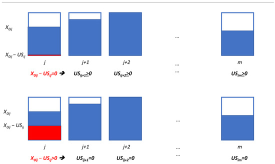
Figure 1. FIFO logic for the assignment of the initial stock.

The goal of these constraints is to separate the quantity of SKU i removed from bin j assigned to SKU i as initial stock ($U{S}_{ij}$), from the one assigned to bin j due to production ($U{P}_{ij}$).

Finally, the following additional constraints are added to the model:

$$U{S}_{ij}\le X_{0ij}i=1, 2,\dots , nj=1, 2,\dots , m$$

(13)

Constraint (13) guarantees that the quantity $U{S}_{ij}$ of SKU i picked from bin j is not greater than the quantity $X_{0ij}$ of the initial stock of SKU i assigned to bin j.

$$U{S}_{ij}\le C_{ij}{\sigma }_{ij}^{S}i=1, 2,\dots , nj=1, 2,\dots , m$$

(14)

$${\sigma }_{ij}^S\le U{S}_{ij}i=1, 2,\dots , nj=1, 2,\dots , m.$$

(15)

Constraints (14) and (15) set the binary variable ${\sigma }_{ij}^S=1$ whenever $U{S}_{ij}>0$, and 0 otherwise.

$$X_{0ij}-U{S}_{ij}\le C_{ij}{\Delta }_{ij}^{S}i=1, 2,\dots , nj=1 ,2,\dots , m$$

(16)

$${\Delta }_{ij}^S\le X_{0ij}-U{S}_{ij}i=1, 2,\dots , nj=1, 2,\dots , m$$

(17)

Constraints (16) and (17) set the binary variable ${\Delta }_{ij}^S$ equal to 1 whenever bin j has positive residual capacity after picking the quantity $U{S}_{ij}$, and 0 otherwise.

$${\Delta }_{ij}^S+{\sigma }_{is}^S\le 1i=1, 2,\dots , nj=1, 2,\dots , m-1s=j+1, j+2\dots , m$$

(18)

Constraint (18) applies the FIFO logic to the bins used in the assignment of the initial stock. In fact, they guarantee that, if ${\Delta }_{ij}^S=1$, then ${\sigma }_{is}^S=0$ for any bin $s=j+1, j+2\dots , m$. Therefore, no quantity can be picked from any bin $s=j+1, j+2,\dots , m$, i.e., $U{S}_{is}=0$ for any bin $s=j+1, j+2,\dots , m$.

Consider now the application of the FIFO logic to production. We need a set of constraints that guarantee that, given any SKU i and any bin j at which the initial stock of i is assigned, if bin j has some residual quantity of SKU i after having picked the quantity $U{S}_{ij}$ (i.e., ${\Delta }_{ij}^S=1$), then ${\sigma }_{is}^P=0$ for any bin $s=j+1, j+2\dots , m$ at which the production is assigned. Therefore, no quantity $U{P}_{is}$ can be picked from any bin $s=j+1, j+2,\dots , m$, i.e., $U{P}_{is}=0$ for any bin $s=j+1, j+2,\dots , m$ if there are bins related to the initial stock with positive residual quantity (i.e., ${\Delta }_{ij}^S=1$). To obtain this, we introduce the following constraints.

$$U{P}_{ij}\le C_{ij}{\sigma }_{ij}^{P}i=1, 2,\dots , nj=1, 2,\dots , m$$

(19)

$${\sigma }_{ij}^P\le U{P}_{ij}i=1, 2,\dots , nj=1, 2,\dots , m.$$

(20)

Constraints (19) and (20) set the binary variable ${\sigma }_{ij}^P=1$ whenever $U{P}_{ij}>0$, and 0 otherwise.

$${\Delta }_{ij}^S+{\sigma }_{ij}^P\le 1i=1, 2,\dots , nj=1, 2,\dots , m-1s=j+1, j+2\dots , m.$$

(21)

Constraints (21) guarantee the FIFO logic for production. In fact, if ${\Delta }_{ij}^S=1$, then ${\sigma }_{is}^P=0$ for any bin $s=j+1, j+2\dots , m$ at which production is assigned. Therefore, no quantity $U{P}_{is}$ can be picked from any bin $s=j+1, j+2,\dots , m$.

Consider now the application of the FIFO logic to the bins used to assign the quantity produced. We need a set of constraints that guarantee that, given any SKU i and any bin j at which the initial stock and the production of i is assigned, if bin j has some residual quantity of SKU i after having picked the quantities $U{S}_{ij}$ and $U{P}_{ij}$ (i.e., ${\Delta }_{ij}^P=1$), then ${\sigma }_{is}^P=0$ for any bin $s=j+1, j+2\dots , m$. Therefore, no quantity can be picked up from any bin $s=j+1, j+2,\dots , m$, i.e., $U{P}_{is}=0$ for any bin $s=j+1, j+2,\dots , m$. To obtain this, we introduce the following constraints.

$$X_{1ij}\le C_{ij}{\Delta }_{ij}^{P}i=1, 2,\dots , nj=1, 2,\dots , m$$

(22)

$${\Delta }_{ij}^P\le X_{1ij}i=1, 2,\dots , nj=1, 2,\dots , m.$$

(23)

Constraints (22) and (23) set the binary variable ${\Delta }_{ij}^P$ as equal to 1 whenever bin j has positive residual capacity after picking the quantity $U{P}_{ij}$, and 0 otherwise.

$${\Delta }_{ij}^P+{\sigma }_{ij}^P\le 1i=1, 2,\dots , nj=1, 2,\dots , m-1s=j+1, j+2\dots , m$$

(24)

Constraint (24) applies the FIFO logic to the bins used in the assignment of the production. In fact, they guarantee that, if ${\Delta }_{ij}^P=1$, then ${\sigma }_{is}^P=0$ for any bin $s=j+1, j+2\dots , m$. Therefore, no quantity can be picked from any bin $s=j+1, j+2,\dots , m$, i.e., $U{P}_{is}=0$ for any bin $s=j+1, j+2,\dots , m$.

We now prove that this problem is NP-hard by showing that the minimal cost (coverage) 0–1 knapsack problem, which is known to be NP-hard, is a particular case of it.

Theorem 1. 

Problem (1)–(24) is NP-hard.

Proof. 

Consider the simplified version of the problem with $k=0$ only, in which the initial stock of a single SKU must be assigned. The problem (1)–(24) becomes

$$min\sum _{j=1}^m{A}_j{Y}_j$$

(25)

$$\sum _{j=1}^m{X}_j=S$$

(26)

$$X_j\le C_j{Y}_{j}j=1, 2,\dots , m$$

(27)

$$X_j\ge 0 \mathrm{integer}j=1, 2,\dots , m$$

(28)

$$Y_j\in \{0,1\}j=1, 2,\dots , m$$

(29)

By summing up Constraint (27), the following relaxation is obtained:

$$min\sum _{j=1}^m{A}_j{Y}_j$$

(30)

$$S\le \sum _{j=1}^m{C}_j{Y}_j$$

(31)

$$Y_j\in \{0,1\}j=1, 2,\dots , m$$

(32)

The latter problem is the minimal cost (coverage) 0–1 knapsack problem, which is known to be NP-hard (see Martello and Toth [19]).    □

5. A Heuristic Algorithm

In this section, given that the problem is NP-hard, we provide a heuristic algorithm for the solution of the problem, inspired by the current rule of thumb applied by the company. This rule is based on operational procedures, refined over the years, mainly on an experiential basis. Daily, at least four times a day, the logistics area manager and his team update the stock flow data in Microsoft Excel files, obtaining in this way a report of the stock levels and, at the end of the day, the final stock levels. Based on the processed data, they decide how to assign the quantities produced. The decision is based on their experience. The first part of the warehouse, from bin number 1 to bin number 6, is dedicated to high rotation SKUs, while the remaining bins are used for medium- and low-rotation SKUs. Based on the current stock levels, the expected production plan and the orders to be processed, the allocation of the SKUs is done, trying to have as many free bins as possible. Since only one SKU can be stored in each bin, the choice is based on the trade-off between how much SKU production a bin is able to contain, and how quickly it can be emptied, depending on the orders that need to be fulfilled, to make the bin empty for the next allocation. All data, as mentioned, are processed on Excel printouts, while the calculations on the various trade-off scenarios are made by physically inspecting the warehouse. Following this analysis, the sequence of the bins used until the next update is established. Sometimes, the need to provide housekeeping activities emerges in the analysis. The most recurrent example is that of repositioning the pallets at the beginning of the bin. Each bin is used to allocate stock in one direction and is used to remove stock in the other. This promiscuity determines that any bin that has exhausted the space available for stock allocation cannot be used until it is completely emptied from the opposite direction. Repositioning the remaining pallets at the beginning of the bin allows the manager to have new space for stock allocation.

Let us now describe the heuristic we propose, in which three consecutive steps are carried out: Assign, Production and Outbound. Since the company uses the same cost for each bin and SKU, the following is based on having $A_{ij}=1$, for all i and j.

The objective of the first step (Assign) is to minimize the waste of space in the assignment of the initial stock. If the stock of an SKU to be assigned is less than or equal to the capacity available in one or more bins, the logic is to select the available bin which allows us to minimize the difference between the assigned stock and the storage capacity of the bin. However, if the stock to be allocated is greater than the capacity of all available bins, the logic is to choose the bin that allows us to allocate the largest quantity of product; we choose the one with the largest capacity with the aim of minimizing the total number of bins used. This step is described in Algorithm 1.   

Algorithm 1: Assign

Let us now describe the second step (Production) of the heuristic algorithm. This step is very similar to the one used in the previous step. The activity always concerns the assignment of the pallets to the bins; in particular, in this second step we must choose where to place the pallets coming from the production lines—the volume to be managed depends on the production plan and varies from day to day. The goal is again to minimize the waste of warehouse space. In this step, however, we have the additional constraint of filling the bins up to capacity in the first step, to assign the initial stock. Bins are assigned using a dedicated storage policy. Therefore, if in the list of used bins, there is one bin with residual storage capacity, this bin will be the first to be used to allocate production. Again, the idea is to saturate its capacity, which, by definition, cannot be occupied with another SKU. Note that at most one bin can have a positive residual capacity in the first step of the algorithm. This step is described in Algorithm 2.  

Algorithm 2: Production

The third step of the heuristic (Outbound) is related to picking quantities from bins, following the FIFO principle, to satisfy pending orders. It is described in Algorithm 3.

Algorithm 3: Outbound

6. Computational Results

The mathematical model formulated in Section 4 and the heuristic algorithm described in Section 5 were implemented in C++ using Visual Studio 2020. The model was solved by using CPLEX 20.1.0 on an Intel(R) Xeon(R) W-1290P Processor manufactured by Intel Corporation, headquartered in Santa Clara, CA, USA, with CPU @3.70 GHz and 64 GB of RAM. This equipment was sourced by the University of Brescia. A dataset of 108 real-world instances was created using the company’s data from 2022. To allow the reader to replicate the results of the developed approaches, these instances are available at https://github.com/Fepeder/PhD_Thesis_Data.git (accessed on 8 February 2026). For each instance, the optimal solution found by CPLEX and the heuristic solution are compared with the company solution.

To analyze the quality of the solutions, the following performance indicators are taken into account:

-

Total number of bins used at time periods 0 and 1;

-

Computational time (in seconds).

Moreover, we consider another metric to compare the solutions, given by the saturation of the space in the warehouse, at time periods 0 and 1. Even if this metric is not in the objective function of the model, it is important from a practical point of view. To do that, we use the following two indicators:

-

Free space: It expresses the residual capacity of the warehouse, calculated as the sum of the capacity of each unused bin. These bins can be used in the future to allocate any SKU.

-

Remaining space: It expresses the residual capacity of the warehouse, calculated as the sum of the residual capacity of used bins. Partially used bins can be useful in the future to assign the same SKU that is currently allocated to each of them.

Note that both indicators are expressed as a number of pallets.

Figure 2 shows a graphical example of what has just been described: 8, 9, and 10 are three bins, each having a capacity of 240 pallets. Each bin is composed of four parallel rows of 60 pallets each. Bin 8 is not free, but it has remaining space that can be used only to allocate the same SKU in the future. Bin 9 is free, as no SKUs are currently assigned to it. Any SKU can be assigned to it in the future. Finally, bin 10 is neither free nor has remaining free space, as it is completely occupied by SKUs.

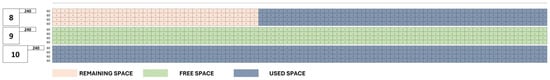
Figure 2. Free space and Remaining space.

In our problem, as mentioned before, free space and remaining space were not included in the objective function of the mathematical model. However, even if they are secondary objectives, they are useful for quantifying usable and unusable (remaining) free space. This is the reason why we computed and evaluated them, to enrich the information provided to the manager on the performance of optimal and heuristic solutions. Instead, although useful and widely used in the literature, indicators such as service level, fill rate, stockout risk, or inventory turnover are not as effective for addressing our problem. In our case, the objective is only the management of internal flows, without considering other aspects that are typical in inventory management problems, such as forecast errors or the picking compliance rate. One line of research development, given the results that emerged, could be to formulate a multi-objective model that also takes these KPIs into account, in order to validate the results already obtained through the heuristic approach.

Let us first show the results in terms of the number of bins used. Figure 3 shows the results obtained, for each of the 108 instances, by the mathematical model (Optimal), the heuristic algorithm (Heur), and the company solution (COM), in terms of the total number of bins used at the time periods 0 and 1.

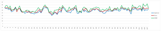
Figure 3. Total number of bins used.

If we look at the total number of bins used in the 108 instances, the optimal solution uses 3103 bins, the heuristic solution 3298, and the company solution 3521 bins. Therefore, the percentage of optimal savings given by the Heuristic is

$${\displaystyle \frac{COM-Heur}{COM-Opt}}=53.35\%,$$

meaning that the heuristic already achieves $53.35\%$ of the benefits of optimization. Since in the instances we used, the cost associated with each bin and SKU is equal to 1, as also adopted by the company, the same results hold in terms of total cost.

Figure 4 shows, for each of the 108 instances, the computational time required to compute the optimal solution and the heuristic solution. The time required by the company is estimated to be 600 s for each instance.

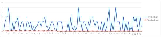
Figure 4. Computational time (sec).

The average results, in terms of the total number of bins and computational time, are summarized in Table 1. On average, the model requires 28.73 bins, the heuristic solution 30.54 bins, while the company 32.60 bins. Therefore, the average number of bins used in the optimal solution is 5.93% less than the number used by the heuristic solution and 11.87% less than the one used by the company. Since the average number of bins used by the heuristic solution is 6.32% less than the one used by the company, a first significant saving could be obtained by the company simply using the heuristic solution. This provides evidence of the importance of formalizing and improving the decision process used by the company. The optimal solution uses approximately 1700 pallets less than the company solution on each day. This implies a significant saving in the annual shuttle cost that the company has to pay to send part of these pallets to external facilities. Instead, the savings of the heuristic solution, with respect to the company solution, is about 50% of the savings obtained using the optimal solution (920 pallets per day).

Table 1. Solution analysis.

	Opt	Heur	COM
Average # of bins	28.73	30.54	32.60
Average time (sec.)	1.44	0.08	600.00

The average computational time to solve the mathematical model to optimality is 1.41 s, to apply the heuristic algorithm it is 0.08 s, while the average time currently taken by the company is 600 s. Given that we have to solve the problem four times a day, and considering a time horizon equal to one year, the time saving that can be obtained by using the model is about 167.61 h in total, and therefore about 39.91 min per day, while it is 167.98 h, and therefore about 39.99 min per day when the heuristic algorithm is applied. The time saving generated by using the model and/or heuristic approach over one year, converted into cost, is approximately 21,600 euros. This considers both the direct costs deriving from carrying out the activity (time in the strict sense) and the indirect costs deriving from the possible standardization of the process.

These results clearly show the advantage of using the model and the heuristic algorithm with respect to the company solution. Moreover, the model is able to achieve a significant reduction in the average number of bins with respect to the heuristic solution, in a computational time that is comparable with the one required by the heuristic algorithm.

The presented heuristics could be easily implemented within any warehouse management system. In our specific case, a custom report was developed in the SAP management system. Whenever flow analysis is required, real-time data on existing stock, production to be allocated, and orders to be fulfilled (which were previously extracted and then processed only in Excel) are currently used to build instances of the problem, that are solved using the proposed heuristic algorithm code.

We now perform some additional analyses to better understand the results we obtained. In Figure 5 we compare the optimal solution with the company solution in terms of how many bins are saved. The comparison shows that the optimal solution uses up to eight bins less than the company solution in about 8.3% of the instances, up to four bins less in $46.3\%$ of the instances, and up to one bin less in 98.1% of the instances. Finally, in only two cases (about 1.8% of the instances) is the number of bins the same. Figure 6 shows the same type of analysis when we compare the heuristic solution with the company solution. The comparison shows that, in a large part of the instances, the heuristic solution uses a lower number of bins. In 70 out of 108 instances (64.8%), the difference ranges from minus 5 bins to minus 1 bin. However, in $29.6\%$ of the instances, there is no gap. Finally, the heuristic solution never uses more bins than the company solution. The heuristic approach was designed by studying the business approach. The number of instances without gaps could be representative of the idea of taking care of the operational rules in the optimization approach.

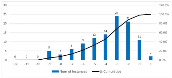
Figure 5. Reduction in the number of bins used in the optimal solution with respect to the company solution.

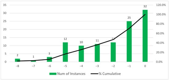
Figure 6. Reduction in the number of bins used in the heuristic solution with respect to the company solution.

In Figure 7, we overlap the two distributions of the reduction in the number of bins moved. The graph shows that the optimal solution is able to have a greater impact on the reduction in the number of bins than the heuristic solution.

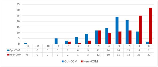
Figure 7. Comparison of the reduction in the number of bins.

Let us now show a more detailed analysis concerning the computational time. Figure 8 shows the Pareto graph of the solution time of the mathematical model. The Pareto chart is a combination of a bar chart and a line chart. The x-axis of the graph contains, in our case, the time intervals to compute the solution. The categories are reported in decreasing order of histogram width. Meanwhile, a line represents the cumulative total of individual values in percentage form. We can see that 50% of the instances are solved in 0.1 to 1.1 s. If we move to the following echelon, up to 2.1 s, the percentage increases to 85.18%.

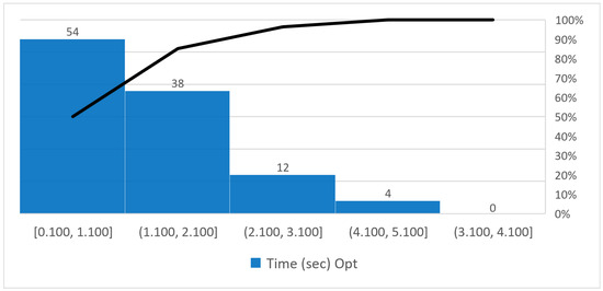
Figure 8. Pareto graph of the solution time of the mathematical model.

Figure 9 shows the Pareto graph of the solution time of the heuristic algorithm: 61.1% instances are solved in 0.052 to 0.072 s.

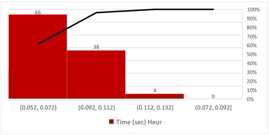
Figure 9. Pareto graph of the solution time of the heuristic algorithm.

Finally, we show the results obtained in terms of free space and remaining space. Even if these goals are not in the objective function, they represent a key driver to understand the capacity of the depot. Indicators are expressed in terms of the number of pallets. Note that the maximum storage capacity of the warehouse is 11,525 pallets. Figure 10 and Figure 11 show a comparison of the free space, in the optimal solution, in the heuristic solution, and in the company solution, at time periods 0 and 1, respectively.

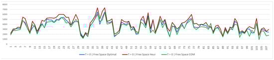
Figure 10. Free space at time period 0.

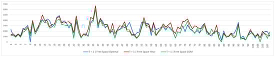
Figure 11. Free space at time period 1.

The free space in the optimal model is very similar to the one in the company’s solution at time period 0, while the heuristic algorithm results in more free space. Conversely, the situation changes when looking at the results obtained in time period 1. The gap between the optimal solution and the company solution becomes wider, and the heuristic solution continues to result in more free space, but is very similar to the optimal solution.

Figure 12 and Figure 13 show the remaining space, related to bins that are just partially used and that can be used in the future only to assign the same SKU that is currently assigned to each of them. We can note that, as is the case for free space, the heuristic solution is better than both the optimal and company solutions—for this KPI, a greater number of pallets is equal to a greater amount of space not being used effectively.

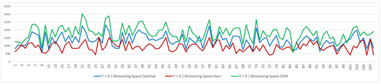
Figure 12. Remaining space at time period 0.

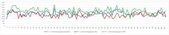
Figure 13. Remaining space at time period 1.

Table 2 shows the average free space and remaining space obtained with the optimal solution, the heuristic solution, and the company solution. Considering the free space, we can notice that the heuristic solution, at time period 0, allows us to have, on average, 446 and 659 more pallets than the optimal solution and the company solution, respectively, which represent $3.87\%$ and $5.71$% of the maximum storage capacity. In time period 1, the heuristic solution has 161 and 391 more pallets, equal to $1.39\%$ and $3.39$% of the maximum storage capacity. Note that the average free space decreases going from time period 0 to time period 1. A part of the efficiency is physiologically lost in the transition from time period 0 to time period 1, due to the fact that the flow rules are both considered at the second time. This is due to how the heuristic solution is designed—the Assign step selects the bin that best fits the quantity to be allocated at each iteration, trying to minimize any waste of space; the production assignment flow and picking quantity flow are both considered at time period 1 and the second one exclusively follows the FIFO picking logic. Concerning the average remaining space at time period 0, the heuristic solution has 420 pallets less than the optimal solution, and 870 pallets less than the company solution. In time period 1, the heuristic solution has 823 pallets less than the company solution and 171 pallets less than the optimal solution. By analyzing these results, it is possible to immediately understand how, for this KPI, there is a gap between the proposed methods and the company solution. The remaining space increases in the transition from time period 0 to time period 1—in addition to the assignment of production at time period 1, the picking of the quantities that must be delivered also takes place. This physiologically leaves bins open, thus generating this unused space which can then be filled with the next flow. The heuristic algorithm achieves better results in terms of free space and remaining space because it was designed to minimize the number of bins and, at the same time, to “choose” the best bin to use in the stock allocation steps. From this perspective, the model is much less constrained because only the total number of bins used is minimized. Starting from a matrix of possible pallet quantities that varies according to the product–stack relationship, it was possible to compare the warehouse occupancy resulting from the two methodologies. In many cases, the total number of stacks used by the heuristic and optimal solutions is similar. The difference in terms of free space and remaining space determines how the selected bins are used. The heuristic algorithm performs better in this regard. As already mentioned, developing a model that adds these two KPIs to the objective function could be an interesting topic for further study. Another point to consider is that, in the heuristic algorithm, the picking sequence is dictated by the imposed rules, while in the model, the order is just the increasing numerical order. At an operational level, there is no difference, but developing these two aspects within the model in this way would increase the difficulty, both in terms of formulation and computability, and would therefore distance itself from ease of application in real-world contexts. In this regard, we have also defined its execution over two periods, on average four times a day, but the application could also be performed over multiple periods and on separate flows. Identifying the warehouse situation at a certain time of day allows for the results of the various steps to be easily evaluated. The assignment phase will return a solution to be compared with the warehouse situation; a pallet “cleaning phase” can be performed if useful, or the production assignment phase can be proceeded with based on the current stock situation. This flexibility of adoption offers the ability to analyze the best option at any time and correlate it with the status of actual operations, thus proving a valuable tool for managerial decisions.

Table 2. Average Free space and Remaining space.

Time 0	Opt	Heur	COM
Average free space	3572.27	4018.10	3359.56
Average remaining space	1358.62	938.06	1808.20
Time 1	Opt	Heur	COM
Average free space	2314.35	2475.46	2084.84
Average remaining space	2580.09	2408.29	3231.32

7. Discussion

In this paper we studied the stock allocation problem with FIFO picking constraints. While classical stock allocation problems are defined over one time period, our problem is defined over two time periods, the first related to the assignment of the initial stock and the second related to the assignment of production and the picking operations. Moreover, the FIFO logic is applied when picking is performed.

7.1. Implications for Theory

Given these two main features of our problem, we formulated a new integer linear programming model able to capture the complex constraints needed to guarantee the FIFO logic. From the theoretical point of view, we also proved that this problem is NP-hard, justifying in this way the use of heuristic algorithms.

7.2. Implications for Practice

The new integer linear programming model was tested on instances built on the data of a leading Italian mineral water bottling company. The computational results showed that the problem can be easily solved to optimality on these instances. Therefore, even if the problem is in general NP-hard, optimal solutions can be applied in practice. Moreover, a heuristic algorithm was designed on the basis of the rule of thumb applied by the company. The computational results showed that this heuristic algorithm is effective and able to provide good results with respect to KPIs pertaining to residual space, which were not included in the objective function of the optimization model.

7.3. Limitations of the Study and Future Research Directions

The problem studied the optimization of logistics flows starting from the existing storage logic (bin management). This structural element represents the warehouse as a black box, where space allocation is not linked to specific factors and indicators (safety stock, inventory rotation, EOQ, etc.) but simply to the optimal occupation of the available space. The introduction of more modern storage systems (racking) could be accompanied by the study of more modern storage policies, such as WMS, slotting algorithms, material flow systems, or smart warehousing. Future research could be devoted to studying a multi-objective model in which all these different KPIs can be balanced. Moreover, the current approach is based on the assumption of a given layout. Dynamic models, able to adapt the layout on the basis of the stock flows, could be formulated and solved. Finally, more general situations could be studied: different product types (e.g., high volume or high value), over more than two time periods, with different assumptions on bin cost, and including forecasting errors in production or demand.

References

- Gu, J.; Goetschalckx, M.; McGinnis, L. Research on warehouse operation: A comprehensive review. Eur. J. Oper. Res. 2007, 177, 1–21. [Google Scholar] [CrossRef]
- Guerriero, F.; Musmanno, R.; Pisacane, O.; Rende, F. A mathematical model for the Multi-Levels Product Allocation Problem in a warehouse with compatibility constraints. Appl. Math. Model. 2013, 37, 4385–4398. [Google Scholar] [CrossRef]
- Medrano-Zarazúa, L.; Saucedo-Martínez, J.; Bolaños-Zuñiga, J. Storage Location Assignment Problem in a Warehouse: A Literature Review. In Proceedings of the International Conference on Computer Science and Health Engineering; Springer: Cham, Switzerland, 2022; pp. 15–37. [Google Scholar]
- Heragu, S.; Du, L.; Mantel, R.; Schuur, P. Mathematical model for warehouse design and product allocation. Int. J. Prod. Res. 2005, 43, 327–338. [Google Scholar] [CrossRef]
- Hausman, W.; Schwarz, L.; Graves, S. Optimal storage assignment in automatic warehousing systems. Manag. Sci. 1976, 22, 629–638. [Google Scholar] [CrossRef]
- Fumi, A.; Scarabotti, L.; Schiraldi, M. Minimizing Warehouse Space with a Dedicated Storage Policy. Int. J. Eng. Bus. Manag. 2013, 5, 21. [Google Scholar] [CrossRef]
- Hou, J.; Wu, Y.; Yang, Y. A model for storage arrangement and re-allocation for storage management operations. Int. J. Comput. Integr. Manuf. 2010, 23, 369–390. [Google Scholar] [CrossRef]
- Battista, C.; Fumi, A.; Laura, L.; Schiraldi, M. Multiproduct slot allocation heuristic to minimize storage space. Int. J. Retail. Distrib. Manag. 2014, 42, 172–186. [Google Scholar] [CrossRef]
- Goetschalckx, M.; Ratliff, H. Shared Storage Policies Based on the Duration Stay of Unit Loads. Manag. Sci. 1990, 36, 1120–1132. [Google Scholar] [CrossRef]
- Lee, M.; Elsayed, E. Optimization of warehouse storage capacity under a dedicated storage policy. Int. J. Prod. Res. 2005, 43, 1785–1805. [Google Scholar] [CrossRef]
- Larson, T.; March, H.; Kusiak, A. A heuristic approach to warehouse layout with class-based storage. IIE Trans. 1997, 29, 337–348. [Google Scholar] [CrossRef]
- de Koster, R.; Le-Duc, T.; Roodbergen, K. Design and control of warehouse order picking: A literature review. Eur. J. Oper. Res. 2007, 182, 481–501. [Google Scholar] [CrossRef]
- Frazele, E.; Sharp, G. Correlated assignment strategy can improve any order-picking operation. Ind. Eng. 1989, 21, 33–37. [Google Scholar]
- Frazelle, E. Stock Location Assignment and Order Picking Productivity; Georgia Institute of Technology: Atlanta, GA, USA, 1989. [Google Scholar]
- Jarvis, J.; McDowell, E. Optimal Product Layout in an Order Picking Warehouse. IIE Trans. 1991, 23, 93–102. [Google Scholar] [CrossRef]
- Brynzér, H.; Johansson, M. Storage location assignment: Using the product structure to reduce order picking times. Int. J. Prod. Econ. 1996, 46, 595–603. [Google Scholar] [CrossRef]
- Ashayeri, J.; Gelders, L. Warehouse design optimization. Eur. J. Oper. Res. 1985, 21, 285–294. [Google Scholar] [CrossRef]
- Gu, J.; Goetschalckx, M.; McGinnis, L. Solving the forward-reserve allocation problem in warehouse order picking systems. J. Oper. Res. Soc. 2010, 61, 1013–1021. [Google Scholar] [CrossRef]
- Martello, S.; Toth, P. Knapsack Problems: Algorithms and Computer Implementations; John Wiley & Sons, Inc.: Hoboken, NJ, USA, 1990. [Google Scholar]
Disclaimer/Publisher’s Note: The statements, opinions and data contained in all publications are solely those of the individual author(s) and contributor(s) and not of MDPI and/or the editor(s). MDPI and/or the editor(s) disclaim responsibility for any injury to people or property resulting from any ideas, methods, instructions or products referred to in the content. |
© 2026 by the authors. Licensee MDPI, Basel, Switzerland. This article is an open access article distributed under the terms and conditions of the Creative Commons Attribution (CC BY) license.