Abstract
In this work, the feasibility of simulating the thermal inactivation of Brochothrix thermosphacta in beef during heating processing based on hyperspectral imaging (HSI) in the wavelength range of 400–1000 nm was investigated. The Weibull and modified Gompertz kinetic models for the thermal inactivation of B. thermosphacta in beef heated in the range 40–60 °C were developed based on the full wavelength, featured spectral variables, and their principal component scores of HSI information, respectively. Notably, the specific wavebands at 412 nm and 735 nm showed a strong correlation with the surviving B. thermosphacta population during the beef heating process. The partial least squares regression models had a satisfactory ability in quantifying B. thermosphacta in beef, with an Rv2 and RMSE of 0.826 and 0.341 log CFU/g, respectively. Furthermore, the Weibull model coupled with the HSI at 735 nm was suitable for kinetic modeling of the thermal inactivation of B. thermosphacta in beef, with an R2 value of 0.937. Consequently, this work suggests the potential of the HSI technique for quantifying and monitoring microbes in meat during heating and can be applied for the thermal inactivation kinetic modeling of microorganisms.
1. Introduction
Microbial contamination, including pathogenic and spoilage bacteria, is one of the most important factors of foodborne diseases caused by eating meat products [1,2]. Beef is a nutrient-rich ideal medium for the growth of different microbes like Brochothrix thermosphacta, Pseudomonas spp., and Enterobacteriaceae [3]. B. thermosphacta is known as a common dominant spoilage bacterium in beef due to its putrefactive capability of producing volatile organic compounds, causing cheesy or sour odors [4,5]. Its growth and reproduction not only spoil meat but also pose a potential risk to human health by producing biogenic amines, especially in cases of significant contamination [6,7]. It is essential for beef quality and potential health threats to monitor B. thermosphacta loads in beef products during processing. Heating treatment is widely used for meat processing [8] and aims to strengthen sensory properties and destroy microorganisms in order to enable meat safety and extend meat shelf-life [9,10]. Thermal treatment has some negative effects on meat products, such as the loss of nutrients [11], poor quality attributes [12], and excessive energy consumption, posing the challenge of fully inactivating microorganisms while retaining original sensory quality and nutrients.
To address the above challenge, many researchers have focused on the specific thermal time and temperature obtained by constructing predictive survival models of bacteria. Weibull and Gompertz kinetic models are widely used in microbial prediction to describe growth processes over time. These two approaches are complementary and can be utilized to model complex dynamic systems. Thus, the thermal inactivation models of Listeria monocytogenes in crab meat were explored [13], and a Z-value of 4.9 °C was reported. Furthermore, the thermal inactivation of Shiga toxin-producing Escherichia coli in ground beef with varying fat content was researched [14], and the ranges of the obtained D-values were 15.93–11.69, 1.15–1.12, and 0.14–0.09 min at 55, 60, 65, and 68 °C, respectively. It was observed that the previous research usually used the traditional plate count method to build thermal inactivation models for monitoring the surviving bacteria in meat during heating. Given the rapid technological progress of machine-led and intelligent food production lines, the time-consuming, laborious, and destructive culture-based method was obsolete [15]. The latest nondestructive technologies must be utilized for bacterial detection to satisfy the development demand of the meat industry.
Hyperspectral imaging (HSI) is a promising technology for rapid nondestructive determination, which can simultaneously acquire both the spatial and spectral information of samples [16]. HSI can identify the spectral features related to the fundamental vibrations of molecular overtones and combinations; thus, it is widely applied for the quantitative and qualitative analysis of quality parameters (e.g., color, moisture content, and microbial loads) during food processing [17], for example, the quantified color (Rp2 = 0.890) and moisture content (Rp2 = 0.869) of beef during microwave heating based on HSI [18], and HSI was used to construct PLSR quantitative models of Salmonella Typhimurium (Rp2 = 0.9687) and Escherichia coli (Rp2 = 0.9687) in pork ultrasonicated for 10, 20, and 30 min [19]. Although the application of the HSI technology in the thermal processing of meat was emphasized in several recent studies [20,21], few studies have combined HSI with thermal inactivation models to explore the thermal inactivation state of microorganisms in meat during heating in order to precisely determine the thermal parameters for achieving commercially sterile meat products.
Therefore, to explore the feasibility of simulating the thermal inactivation of B. thermosphacta in beef during heating based on HSI, the aims of this study are to (i) investigate the hyperspectral spectral characteristic in the 400–1000 nm spectral range of beef inoculated with B. thermosphacta during heating at 40, 45, 50, 55, and 60 °C; (ii) construct thermal inactivation models for the quantitative prediction of B. thermosphacta in beef based on HSI; and (iii) perform kinetic modeling for the thermal inactivation of B. thermosphacta in beef heated in the range 40–60 °C based on the feature HSI information extracted by three methods, and perform a comparison with those models based on the conventional plate count method.
2. Materials and Methods
2.1. Inoculum Preparation
B. thermosphacta (strain number: ACCC03872) was stored at 4 °C in the laboratory refrigerator until use (College of Food Science and Technology, Nanjing Agricultural University, Nanjing, Jiangsu, China). The bacterial cultures were obtained by incubating B. thermosphacta on nutrient agar at 30 °C for 24 h, followed by subculturing under the same conditions. For the sake of bacterial suspensions, the cultures were washed and suspended with a sterile saline solution (0.85% NaCl w/v) to a cell level of approximately 107–108 CFU/mL (OD600 = 0.39). The well-prepared bacterial suspensions were applied as inoculum to the beef samples.
2.2. Sample Preparation and Inoculation
Beef samples (Longissimus dorsi) purchased from the local supermarket were transported to the laboratory in an average time of 30 min. Beef was trimmed to remove the fat or connective tissue. After wiping with ethanol (75% v/v), beef samples were treated with ultraviolet light (UV-C) for 30 min. Then, samples were aseptically divided into 4 cm × 4 cm × 2 cm (length × width × thickness) pieces using a sterile knife, thoroughly mixed with the inoculum for 3 min, and naturally dried on the sterile table for 30 min to make bacteria adhere to meat surfaces. The inoculated samples were heat-sealed in polyethylene plastic bags (0.08 mm in thickness).
2.3. Thermal Inactivation
For the packaged samples, the submerged heating treatments at different temperatures were carried out in a constant temperature water bath (HH-8, Changzhou Guohua Electric Appliance Co., Ltd., Changzhou, China). At each time interval, 10 samples were taken for the heating treatment, particularly, at 24 min intervals at 40 °C for 120 min, at 12 min intervals at 45 °C for 60 min, at 6 min intervals at 50 °C for 30 min, at 3 min intervals at 55 °C for 15 min, and at 0.5 min intervals at 60 °C for 2.5 min. Thus, 60 samples were obtained for each temperature treatment; a total of 300 samples were used for this experiment. The come-up time based on the pre-experiments was excluded from the total heating time. At each time interval, 10 samples were taken for the heating treatment. Immediately, the heated samples were plunged into the ice bath to prevent further inactivation. The HSI data collection and surviving B. thermosphacta enumeration for beef samples were subsequently performed. Finally, a total of 300 samples were used for this experiment.
2.4. Enumeration of Surviving B. thermosphacta
The conventional plate count method was applied for the enumeration of surviving B. thermosphacta in heated samples. About 5 g of each beef sample was transferred to a sterile homogenization bag with 45 mL of 0.85% NaCl autoclaved solution and homogenized for 2 min. Serial 10-fold dilutions were made, and 0.1 mL were plated on streptomycin thallous acetate actidione agar (STAA) containing the STAA selective supplement. Then, the STAA plates were incubated at 30 °C for 48 h. The enumeration of surviving B. thermosphacta was described as ten-based logarithm values (log CFU/g).
2.5. Modeling B. thermosphacta Inactivation in Beef
2.5.1. Mathematical Models of B. thermosphacta Inactivation
The inactivation curves of B. thermosphacta were described using primary models, including the Weibull model [22] and modified Gompertz model [23]. Secondary models were used to describe the effect of temperature on the inactivation parameters. For the Weibull model (Equation (1)), a suitable secondary model for the parameter δ was expressed as Equation (2). The parameters and obtained from the modified Gompertz model (Equation (3)) were fitted with Equations (4) and (5), respectively.
In which and are the bacterial population or hyperspectral characteristic values (log CFU/g or none) at time 0 and actual time t (min), respectively; is the time parameter or time of first decimal reduction; is the shape parameter; is the temperature (°C); and and are model parameters.
where , , , and are the same as expressed above; is the asymptotic survival ratio reached at the end; is the maximum inactivation rate (time−1); is the shoulder length (min); min is the theoretical minimum temperature for inactivation (°C); and , , and are model parameters.
2.5.2. One-Step Nonlinear Regression
Primary and secondary models were constructed simultaneously by a one-step kinetic analysis. All the inactivation data were assembled and analyzed simultaneously using the nonlinear regression procedure (FITNLM) in MATLAB R2016a software (The Mathworks, Inc., Natick, MA, USA). This approach, utilizing advanced computational tools for simultaneous parameter estimation, is integral to the continuing research aimed at enhancing our understanding and predictive capabilities regarding microbial inactivation in food safety, particularly through the integration of hyperspectral imaging with kinetic modeling. Based on nonlinear least squares optimization algorithms, the FITNLM procedure was designed to estimate inactivation parameters in primary and secondary models, simultaneously. Inactivation parameters of the Weibull and modified Gompertz models were expressed as Equation (6) and Equation (7), respectively.
2.6. Hyperspectral Imaging (HSI) Data Acquisition and Preprocessing
Prior to B. thermosphacta enumeration, a hyperspectral reflectance imaging system (SPECIM, Oulu, Finland) in the range of 400–1000 nm was used to acquire the HSI data of beef samples. The system was composed of a CCD camera with a spectral resolution of 2.8 nm, a 150 W halogen lamp, a sample delivery platform, and a computer with data acquisition software. The entire hyperspectral imaging system was enclosed in a black box to eliminate the influence of external light during data acquisition.
The working parameters of the HSI system were as follows: The lamp was fixed at around a 45° angle over the sample and positioned at a distance of about 30 cm from the sample; the camera exposure time was set as 3 ms; and the speed of the sample delivery platform was 7.23 mm/s. The size of collected hyperspectral images of beef samples was 804 × 440 pixels, retaining the spectral information of 420 available bands in the range of 400–1000 nm.
The camera dark currents and external factors have an impact on the collected images, so it is necessary to calibrate raw hyperspectral images. Calibrated images were acquired by a white reference image collected from a Teflon whiteboard (99% reflectivity) and a dark reference image collected by covering the camera lens with its black opaque cap. The calibrated image was calculated by Equation (8):
where is the calibrated image; is the raw image; is the white reference image; and is the dark reference image.
Spectral extraction was conducted in the MATLAB R2016a software. The region of interest (ROI) based on the whole sample surface was isolated from the background by the threshold segmentation algorithm. The mean spectral values of all pixels in each ROI were considered as spectral information of each beef sample.
To minimize the noise interference from the instrument itself and the surroundings, the extracted spectra were preprocessed. Several algorithms, including orthogonal signal correction (OSC), standard normal variate (SNV), and multiplicative scattering correction (MSC), were compared.
2.7. Modeling of Spectral Information from HSI
2.7.1. Quantitative Modeling of Surviving B. thermosphacta
Partial least squares regression (PLSR) and support vector machine regression (SVMR) were used for the quantitative prediction of surviving B. thermosphacta. The PLSR model, as a multilinear regression model, can identify linear relationship between observations and predictions [24]. SVMR is a supervised learning method using the concept of decision planes with an excellent generalization ability, which can build nonlinear relationships between lossless signal rationalization indicators [25]. Both are widely applied in the regression of spectral data.
In the work, 300 spectral data were randomly divided into a calibration dataset and validation dataset at a ratio of 3:1 using the Kennard–Stone algorithm in MATLAB R2016a software. Then, PLSR and SVMR prediction models were established based on the preprocessed full-band spectral data. The predicted performance of different quantitative models was compared.
2.7.2. Survival Kinetic Modeling of B. thermosphacta by HSI
In this work, three methods were adopted to build survival kinetic models of B. thermosphacta based on HSI information (Figure 1):
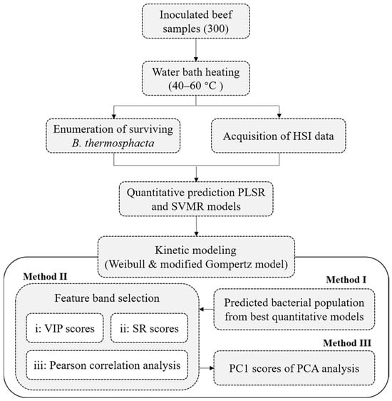
Figure 1.
Flowchart of quantitative prediction and kinetic modeling for the thermal inactivation of B. thermosphacta in beef using HSI.
Method I: The surviving bacterial population predicted by the above optimal quantitative models (PLSR or SVMR model) was treated as input values to the above mathematical models describing the thermal inactivation of B. thermosphacta.
Method II: The feature spectra reflecting the microbial population were used for the construction of the survival model of B. thermosphacta. Hyperspectral data inevitably contains plenty of redundant and useless information, which affects information extraction, adds the burden of data processing, and easily makes models less effective and stable. Therefore, it is necessary to select feature bands such as variable importance in the projection (VIP), selectivity ratio (SR), Pearson correlation analysis, and continuous projection algorithm. Among them, both VIP and SR scores depend on the PLSR model to measure the importance of wavelength variables to the predicted variables. Generally, the VIP score is taken as 1.0 and recognized as feature bands when the VIP is higher than 1.0. And a higher SR score means that the band is more important, and the contribution is the greatest to the model [26]. In addition, the correlation between the whole wavelengths and bacterial populations could be judged by a Pearson correlation analysis. The spectral values at the band with the largest correlation coefficient have the strongest correlation with the bacterial concentration [27]. Method II would use VIP scores, SR scores, and a Pearson correlation analysis to screen the feature bands, and the spectral values at the selected characteristic bands would be substituted into the above mathematical models for survival kinetic modeling.
Method III: The survival kinetic model of B. thermosphacta was constructed based on the first principal component (PC1) of the full-band HSI data. A principal component analysis (PCA) could also compress hyperspectral data to reduce data redundancy and improve the accuracy and stability of models [28]. PC1 could be obtained by the PCA, which could interpret the most spectral information. Therefore, Method III used PC1 as the input values of the survival function of B. thermosphacta to construct its survival kinetic model.
2.8. Evaluation of Survival Models
It is essential to evaluate the performance of quantitative models, which directly determine the accuracy of survival kinetic models. Generally, the performance of quantitative prediction models is evaluated by the coefficients of determination in calibration (Rc2) and validation (Rv2), the corresponding root mean square error (RMSEC and RMSEV), and the ratio of performance to deviation (RPD) [29].
The goodness of fit of survival kinetic models was assessed by the coefficient of determination (R2) and root mean square error (RMSE) [30]. In addition, the Akaike Information Criteria (AIC) can also help to judge the goodness of fit for the model. A model with a low AIC can perform better in prediction.
2.9. External Validation of Survival Kinetic Models
The survival kinetic models were validated by two extra experiments at 40 °C for 120 min (30 samples) and 60 °C for 2.5 min (30 samples). In order to compare the difference between the observations and predictions of survival kinetic models based on validation experiments at 40 °C and 60 °C, the accuracy ( Equation (9)) and bias (, Equation (10)) factors proposed elsewhere [31] were taken into account. When both and are close to one, the growth model is highly reliable.
In Equations (9) and (10), and represent the predicted and experimental values, respectively; is the total number of the experimental data points.
3. Results and Discussion
3.1. Analysis of Spectral Features
Figure 2 shows the mean reflectance spectra of beef samples at different heating times under different temperatures. The general trends of spectra at different temperatures were similar and the spectral values increased gradually with increased heating time, which was similar to the trends of reflectance spectra of beef slices pretreated with drying at different temperatures [32]. This trend may be associated with factors such as protein, water loss, and color change.
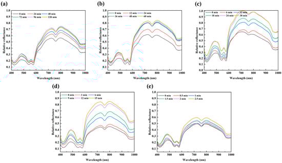
Figure 2.
Mean spectra of beef samples at different heating times under different temperatures ((a): 40 °C; (b): 45 °C; (c): 50 °C; (d): 55 °C; and (e): 60 °C).
As seen in Figure 2, several characteristic peaks and valleys can be highlighted in the 400–1000 nm range. An evident valley around 420 nm was related to the Soret absorption, resulting from the porphyrin compounds [33]. The bands at approximately 490, 545, and 580 nm were associated with metmyoglobin [34], oxymyoglobin [35], and respiratory pigments (e.g., myoglobin, deoxymyoglobin, and hemoglobin) [36], respectively. Two absorption bands at 760 and 970 nm were, respectively, correlated with the third and second overtone O–H stretching, corresponding to the water absorption [37,38]. The presence of characteristic peaks in mean spectra indicated the possibility of using HSI information to determine the variations in protein and water content of beef during heating. Liu et al. [18] have investigated HSI (400–1000 nm) to correlate the mean spectra of beef samples and moisture content and color (L*, a*, and b*) during microwave treatment and demonstrated the ability of HSI for monitoring the changes in some quality parameters during microwave heating. It is known that the reduction in microbial counts of beef samples during heat treatment accompanied changes in quality parameters such as moisture and protein. Thus, bacterial populations might be indirectly quantified by clarifying the correlations between bacterial populations and the protein or water content of beef samples during heating.
3.2. Quantitative Prediction of Surviving B. thermosphacta by HSI
The mean reflectance spectra were used to construct quantitative prediction models of surviving B. thermosphacta by PLSR and SVMR (Table 1). In terms of untreated full-band spectra in the 400–1000 nm range, the overall prediction results were roughly acceptable. The Rv2 of PLSR and SVMR were, respectively, 0.780 and 0.775, and the corresponding RMSEV were, respectively, 0.341 log CFU/g and 0.354 log CFU/g. After preprocessing, the predicted accuracy of both PLSR and SVMR models was slightly but insignificantly improved. As for PLSR models, the MSC algorithm provided the best modeling performance with Rv2 = 0.826, RMSEV = 0.341 log CFU/g, and RPD = 2.415. The SNV algorithm in SVMR models performed best with an Rv2 of 0.804, RMSEV of 0.354 log CFU/g, and RPD of 2.275. Apparently, the MSC-PLSR model presented the optimal capability for predicting surviving B. thermosphacta.

Table 1.
PLSR and SVMR models of surviving B. thermosphacta in heated beef samples based on full-band spectra.
3.3. Survival Kinetic Modeling of B. thermosphacta by the Plate Count Method
The traditional plate count method, a gold standard method for bacterial detection, was used as a reference method to construct Weibull and Modified Gompertz models for the survival kinetics of B. thermosphacta. Figure 3 exhibits the heat survival curves of B. thermosphacta at different temperatures based on the plate count method. In the temperature range of 40–60 °C, the populations of B. thermosphacta initially declined sharply and then decreased very slowly with increased time, with the microbial reductions in two orders of the magnitude [39]. The deactivation degree of B. thermosphacta relied on temperature and the holding time at that temperature. Overall, the survival curve had an insignificant shoulder effect and displayed a nonlinear downward region followed by pronounced tailing. It indicated that the heat processing conditions for B. thermosphacta should be determined by the nonlinear rather than linear equations to avoid considerable errors. Nevertheless, existing research have not yet provided a satisfactory explanation for the phenomenon of the shoulder effect and tailing [40].
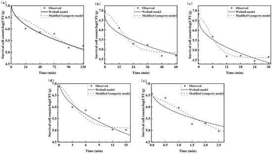
Figure 3.
Heat survival curves of B. thermosphacta at different temperatures based on the plate count method ((a): 40 °C; (b): 45 °C; (c): 50 °C; (d): 55 °C; and (e): 60 °C).
Table 2 records survival parameters fitted with Weibull and modified Gompertz models. All estimated parameters, other than C2, were statistically significant (p < 0.05). Like all inverse problems, the nonlinear regression was not able to ensure all parameters were accurate [41]. The shape parameter of the Weibull models was independent on temperature and estimated as 0.749 ( < 1), indicating that all survival curves were concaved downward [42]. The great performance of the Weibull model was proven by an RMSE of 0.243 log CFU/g, R2 of 0.921, and AIC of −78.186. As for the modified Gompertz model, the minimum survival temperature (Tmin) was predicted as 36.395 °C. In addition, the RMSE, R2, and AIC corresponded to 0.242 log CFU/g, 0.929, and −78.434, respectively. Results suggested that both the Weibull model and modified Gompertz model were appropriate to describe the survival kinetics of heat treated B. thermosphacta.
Table 2.
Survival kinetic parameters of B. thermosphacta in beef estimated by Weibull and modified Gompertz models using the plate count method.
3.4. Different Survival Kinetic Modeling Methods of B. thermosphacta
3.4.1. Survival Kinetic Modeling of B. thermosphacta by Method I
The survival kinetic modeling was conducted based on the predictions of B. thermosphacta from the best MSC-PLSR model (Method I), as shown in Table 3. Similarly, parameters, except C2, fitted by the Weibull and modified Gompertz models differed significantly from zero (p < 0.05), and the of 0.481 and Tmin of 36.009 °C were nearly identical to those by the traditional plate count method. The difference was that the prediction accuracy of the modified Gompertz model (R2 = 0.864, RMSE = 0.256 log CFU/g, and AIC = −73.919) was acceptable but lower than the Weibull model (R2 = 0.922, RMSE = 0.194 log CFU/g, and AIC = −91.699) by Method I and models by the plate count method. It indicated that the Weibull model was extremely accurate when applied for the description of the individual survival curves [43].
Table 3.
Estimated parameters of the thermal inactivation models for B. thermosphacta in beef based on predicted colony counts from HSI (Method I).
3.4.2. Survival Kinetic Modeling of B. thermosphacta by Method II
The Weibull model by Method I was relatively accurate but had the obvious disadvantage of the need for the construction of PLSR models, which undoubtedly increased the computational effort and the risk of error accumulation. So, Method II directly fitted the thermal inactivation curves based on the feature bands reflecting the contents of B. thermosphacta. Figure 4 shows the VIP (Figure 4a) and SR scores (Figure 4b) from the MSC-PLSR model, and the Pearson correlation coefficients (Figure 4c) between the surviving B. thermosphacta population and HSI data. The bands at 412 nm and 735 nm, respectively, showed the largest VIP (>1) and SR scores, and the band at 484 nm had the strongest correlation with the surviving B. thermosphacta population. The results for thermal inactivation models built by the above three bands are listed in Table 4. Both Weibull and modified Gompertz models obtained using the 412 nm wavelength were unsatisfactory due to the relatively low predictive performance with the R2 of 0.753 and 0.676, respectively. The models obtained with the HIS data from 735 nm and 484 nm had a good predictive ability, with the R2 from 0.873 to 0.937, RMSE from 0.029 to 0.037, and AIC from −204.592 to −191.115. Among them, the model based on feature spectral values at 735 nm performed best, and its R2 and Tmin were, respectively, 0.937 and 36.471 °C, comparable to models by the plate count method. A similar situation to that of Method I was that the predictive accuracy of all Weibull models was higher than that of the modified Gompertz models at three different feature bands.
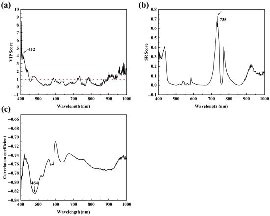
Figure 4.
Results for the selection of feature wavelengths (a) variable importance in projection (VIP) scores and (b) selectivity ratio (SR) scores calculated by the PLSR; (c) Pearson correlation coefficients between B. thermosphacta population and spectral values.
Table 4.
Estimated parameters of the thermal inactivation models for B. thermosphacta in beef based on feature spectral values from HSI (Method II).
3.4.3. Survival Kinetic Modeling of B. thermosphacta by Method III
Although the individual characteristic band had been screened in Method II for survival kinetic modeling of B. thermosphacta, the information contained in the single band was limited. The PCA for full-band spectra in 400–1000 nm was conducted to gain the PC1 fully representing the original spectral information, which allowed for a noticeable reduction in the dimensionality of the HSI data while retaining more information about the loads of microorganisms [44]. Survival kinetic models were developed based on the gained PC1, accounting for 92.3% of the spectral variability (Table 5). As for the model performance, the R2, RMSE, and AIC of the Weibull model were 0.918, 3.450, and 80.998, respectively, indicating a good predictive ability. And the corresponding evaluation results for the modified Gompertz model were 0.855, 4.700, and 99.549, with the Tmin of 36.527 °C close to that by the plate count method. Obviously, the Weibull model was still more accurate than the modified Gompertz model.
Table 5.
Estimated parameters of the thermal inactivation models for B. thermosphacta in beef based on PC1 scores of spectra from HSI (Method III).
3.4.4. Secondary Model of B. thermosphacta
Figure 5 depicts the effect of temperature on the Weibull and modified Gompertz kinetics parameters of B. thermosphacta inactivation. fitted with Weibull models was the scale parameter and decreased linearly with increased temperature (Figure 4a). The maximum survival rate (Kmin, min−1) and the shoulder length (, min) fitted with the modified Gompertz model showed, respectively, an upward and downward concave when the temperature increased (Figure 4b,c). It was observed that the trend of survival parameters (, Kmin, and ) obtained by the traditional plate count method and HSI (Method I, II, and III) was similar as the temperature increased. However, the difference in magnitude made the curves of the survival parameters obtained from Method II and Method III as a function of temperature somewhat different.
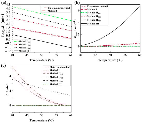
Figure 5.
Effect of temperature on Weibull and modified Gompertz kinetics parameters of B. thermosphacta. (a) relationship between temperature and thermal inactivation parameter δ; (b) relationship between temperature and Kmax; (c) relationship between temperature and L.
A shorter time was needed for the thermal inactivation of bacteria at higher temperatures [43]. There was little available information to explain the dependance of on temperature, which resulted in difficulties related to modeling the temperature effect. The demonstrated explanation included the growth stage of bacteria for the thermal survival research, the recovery media, and so on [45]. However, the relationship between , Kmin, , and temperature could provide a theoretical reference for the thermal inactivation conditions of spoilage bacteria in meat.
3.4.5. Validation of Survival Kinetic Models at Different Temperatures
The extra experimental data at 40 °C and 60 °C were employed to validate the survival kinetic models based on the plate count method and HSI, the results of which are listed in Table 6. It is important to highlight that the HSI values exhibit an inverse correlation with the viable counts following heating: as the viable counts decrease due to thermal inactivation, the HSI values increase. This relationship is critical for understanding the model outcomes. As for the Weibull and modified Gompertz models by the traditional plate count method, the ranges of and were 1.001–1.004 and 1.031–1.046, respectively, suggesting accurate and reliable survival models. The of models based on HSI data (Method I, II735 nm, and III) ranged from 0.999 to 1.004, 1.011 to 1.124, and 0.883 to 1.081, and the corresponding were 1.019–1.041, 1.053–1.129, and 1.174–1.341, respectively. If > 1.30, the model is ‘unacceptable’ [46], which meant that models built by PC1 scores (Method III) were unreliable and unacceptable. It seemed that Method I and II735 nm were more suitable than Method III to build thermal inactivation models based on HSI information.
Table 6.
The accuracy factor () and bias factor () from thermal inactivation models based on extra experimental data at 40 °C and 60 °C.
4. Conclusions
In this study, quantitative prediction and kinetic modeling for the thermal inactivation of B. thermosphacta in beef heated at 40–60 °C were performed using HSI information in the 400–1000 nm spectral range. The results indicated that spectral values of beef samples increased gradually when increasing heating time under different temperatures. The predictive MSC-PLSR model performed best in quantifying B. thermosphacta in beef during heating, with an Rv2, RMSEV, and RPD of 0.826, 0.341 log CFU/g, and 2.415, respectively. In addition, Weibull models based on HSI information extracted by Method I and Method II735 nm were suitable for kinetic modeling of the thermal inactivation of B. thermosphacta in beef, with R2 values of 0.907 and 0.937, which are comparable to those of models based on the traditional plate count method. It was suggested that HSI has the potential to quantify and monitor microbes in meat during heating and can be applied for the thermal inactivation kinetic modeling of microorganisms in meat, which provides the reference for the application of the HSI technique in predictive inactivation models. However, it is important to acknowledge the limitations of this method. While HSI shows promise, it is not yet a replacement for traditional viable plate count methods. Much more research by independent laboratories is necessary to validate the accuracy and reliability of HSI for microbial quantification and inactivation modeling. Instead, it should be employed in conjunction with generally accepted methods, such as plate counting, to ensure robust and accurate assessments of microbial inactivation.
Author Contributions
Author Contributions: Conceptualization, Q.L.; methodology, J.F.G.-M.; software, F.D.; validation, W.L., K.T., and X.L.; writing—original draft preparation, Q.L. and J.F.G.-M.; visualization, X.L. and C.T.; supervision, L.P.; funding acquisition, L.P. and W.L. All authors have read and agreed to the published version of the manuscript.
Funding
This work was supported by the Key Research & Development Program of Jiangsu Province in China (BE2020693), Postdoctoral Fellowship Program of CPSF (Grant Number GZC20232451), the International Science & Technology Cooperation Program of Hainan Province (project No. GHYF2024015) and Priority Academic Program Development of Jiangsu Higher Education Institutions (PAPD).
Institutional Review Board Statement
Not applicable.
Informed Consent Statement
Not applicable.
Data Availability Statement
Data are contained within this article.
Conflicts of Interest
The authors declare no competing financial interest.
References
- Abebe, E.; Gugsa, G.; Ahmed, M. Review on Major Food-Borne Zoonotic Bacterial Pathogens. J. Trop. Med. 2020, 2020, 1–19. [Google Scholar] [CrossRef] [PubMed]
- Majer-Baranyi, K.; Székács, A.; Adányi, N. Application of Electrochemical Biosensors for Determination of Food Spoilage. Biosensors 2023, 13, 456. [Google Scholar] [CrossRef] [PubMed]
- Russo, F.; Ercolini, D.; Mauriello, G.; Villani, F. Behaviour of Brochothrix Thermosphacta in Presence of Other Meat Spoilage Microbial Groups. Food Microbiol. 2006, 23, 797–802. [Google Scholar] [CrossRef]
- Fang, J.; Feng, L.; Lu, H.; Zhu, J. Metabolomics Reveals Spoilage Characteristics and Interaction of Pseudomonas Lundensis and Brochothrix Thermosphacta in Refrigerated Beef. Food Res. Int. 2022, 156, 111139. [Google Scholar] [CrossRef]
- Illikoud, N.; Gohier, R.; Werner, D.; Barrachina, C.; Roche, D.; Jaffrès, E.; Zagorec, M. Transcriptome and Volatilome Analysis During Growth of Brochothrix Thermosphacta in Food: Role of Food Substrate and Strain Specificity for the Expression of Spoilage Functions. Front. Microbiol. 2019, 10, 2527. [Google Scholar] [CrossRef]
- Li, Y.; Zhao, N.; Li, Y.; Zhang, D.; Sun, T.; Li, J. Dynamics and Diversity of Microbial Community in Salmon Slices during Refrigerated Storage and Identification of Biogenic Amine-Producing Bacteria. Food Biosci. 2023, 52, 102441. [Google Scholar] [CrossRef]
- Höll, L.; Hilgarth, M.; Geissler, A.J.; Behr, J.; Vogel, R.F. Metatranscriptomic Analysis of Modified Atmosphere Packaged Poultry Meat Enables Prediction of Brochothrix Thermosphacta and Carnobacterium Divergens in Situ Metabolism. Arch. Microbiol. 2020, 202, 1945–1955. [Google Scholar] [CrossRef]
- Vinnikova, L.; Synytsia, O.; Kyshenia, A. THE PROBLEMS OF MEAT PRODUCTS THERMAL TREATMENT. Food Sci. Technol. 2019, 13, 44–57. [Google Scholar] [CrossRef]
- Hassoun, A.; Cropotova, J.; Rustad, T.; Heia, K.; Lindberg, S.-K.; Nilsen, H. Use of Spectroscopic Techniques for a Rapid and Non-Destructive Monitoring of Thermal Treatments and Storage Time of Sous-Vide Cooked Cod Fillets. Sensors 2020, 20, 2410. [Google Scholar] [CrossRef]
- Hassoun, A.; Ojha, S.; Tiwari, B.; Rustad, T.; Nilsen, H.; Heia, K.; Cozzolino, D.; Bekhit, A.E.-D.; Biancolillo, A.; Wold, J.P. Monitoring Thermal and Non-Thermal Treatments during Processing of Muscle Foods: A Comprehensive Review of Recent Technological Advances. Appl. Sci. 2020, 10, 6802. [Google Scholar] [CrossRef]
- Kong, F.; Tang, J.; Rasco, B.; Crapo, C. Kinetics of Salmon Quality Changes during Thermal Processing. J. Food Eng. 2007, 83, 510–520. [Google Scholar] [CrossRef]
- Rattanathanalerk, M.; Chiewchan, N.; Srichumpoung, W. Effect of Thermal Processing on the Quality Loss of Pineapple Juice. J. Food Eng. 2005, 66, 259–265. [Google Scholar] [CrossRef]
- McDermott, A.; Whyte, P.; Brunton, N.; Bolton, D.J. Thermal Inactivation of Listeria Monocytogenes in Crab Meat. J. Food Prot. 2018, 81, 2003–2006. [Google Scholar] [CrossRef]
- Brar, J.S.; Waddell, J.N.; Bailey, M.; Corkran, S.; Velasquez, C.; Juneja, V.K.; Singh, M. Thermal Inactivation of Shiga Toxin–Producing Escherichia Coli in Ground Beef with Varying Fat Content. J. Food Prot. 2018, 81, 986–992. [Google Scholar] [CrossRef]
- Awang, M.S.; Bustami, Y.; Hamzah, H.H.; Zambry, N.S.; Najib, M.A.; Khalid, M.F.; Aziah, I.; Abd Manaf, A. Advancement in Salmonella Detection Methods: From Conventional to Electrochemical-Based Sensing Detection. Biosensors 2021, 11, 346. [Google Scholar] [CrossRef]
- Wang, K.; Pu, H.; Sun, D. Emerging Spectroscopic and Spectral Imaging Techniques for the Rapid Detection of Microorganisms: An Overview. Comp. Rev. Food Sci. Food Saf. 2018, 17, 256–273. [Google Scholar] [CrossRef] [PubMed]
- Liu, Y.; Pu, H.; Sun, D.-W. Hyperspectral Imaging Technique for Evaluating Food Quality and Safety during Various Processes: A Review of Recent Applications. Trends Food Sci. Technol. 2017, 69, 25–35. [Google Scholar] [CrossRef]
- Liu, Y.; Sun, D.-W.; Cheng, J.-H.; Han, Z. Hyperspectral Imaging Sensing of Changes in Moisture Content and Color of Beef During Microwave Heating Process. Food Anal. Methods 2018, 11, 2472–2484. [Google Scholar] [CrossRef]
- Bonah, E.; Huang, X.; Hongying, Y.; Harrington Aheto, J.; Yi, R.; Yu, S.; Tu, H. Nondestructive Monitoring, Kinetics and Antimicrobial Properties of Ultrasound Technology Applied for Surface Decontamination of Bacterial Foodborne Pathogen in Pork. Ultrason. Sonochemistry 2021, 70, 105344. [Google Scholar] [CrossRef]
- Hassoun, A.; Aït-Kaddour, A.; Sahar, A.; Cozzolino, D. Monitoring Thermal Treatments Applied to Meat Using Traditional Methods and Spectroscopic Techniques: A Review of Advances over the Last Decade. Food Bioprocess Technol. 2021, 14, 195–208. [Google Scholar] [CrossRef]
- Ma, J.; Cheng, J.-H.; Sun, D.-W.; Liu, D. Mapping Changes in Sarcoplasmatic and Myofibrillar Proteins in Boiled Pork Using Hyperspectral Imaging with Spectral Processing Methods. LWT 2019, 110, 338–345. [Google Scholar] [CrossRef]
- Mafart, P.; Couvert, O.; Gaillard, S.; Leguerinel, I. On Calculating Sterility in Thermal Preservation Methods: Application of the Weibull Frequency Distribution Model. Int. J. Food Microbiol. 2002, 72, 1–2. [Google Scholar] [CrossRef] [PubMed]
- Linton, R.H.; Carter, W.H.; Pierson, M.D.; Hackney, C.R. Use of a Modified Gompertz Equation to Model Nonlinear Survival Curves for Listeria Monocytogenes Scott A. J. Food Prot. 1995, 58, 946–954. [Google Scholar] [CrossRef]
- Liu, C.; Chu, Z.; Weng, S.; Zhu, G.; Han, K.; Zhang, Z.; Huang, L.; Zhu, Z.; Zheng, S. Fusion of Electronic Nose and Hyperspectral Imaging for Mutton Freshness Detection Using Input-Modified Convolution Neural Network. Food Chem. 2022, 385, 132651. [Google Scholar] [CrossRef]
- He, J.; Zhu, S.; Chu, B.; Bai, X.; Xiao, Q.; Zhang, C.; Gong, J. Nondestructive Determination and Visualization of Quality Attributes in Fresh and Dry Chrysanthemum Morifolium Using Near-Infrared Hyperspectral Imaging. Appl. Sci. 2019, 9, 1959. [Google Scholar] [CrossRef]
- Baek, I.; Lee, H.; Cho, B.; Mo, C.; Chan, D.E.; Kim, M.S. Shortwave Infrared Hyperspectral Imaging System Coupled with Multivariable Method for TVB-N Measurement in Pork. Food Control 2021, 124, 107854. [Google Scholar] [CrossRef]
- Shicheng, Q.; Youwen, T.; Qinghu, W.; Shiyuan, S.; Ping, S. Nondestructive Detection of Decayed Blueberry Based on Information Fusion of Hyperspectral Imaging (HSI) and Low-Field Nuclear Magnetic Resonance (LF-NMR). Comput. Electron. Agric. 2021, 184, 106100. [Google Scholar] [CrossRef]
- Xie, A.; Sun, J.; Wang, T.; Liu, Y. Visualized Detection of Quality Change of Cooked Beef with Condiments by Hyperspectral Imaging Technique. Food Sci. Biotechnol. 2022, 31, 1257–1266. [Google Scholar] [CrossRef]
- Nicolaï, B.M.; Beullens, K.; Bobelyn, E.; Peirs, A.; Saeys, W.; Theron, K.I.; Lammertyn, J. Nondestructive Measurement of Fruit and Vegetable Quality by Means of NIR Spectroscopy: A Review. Postharvest Biol. Technol. 2007, 46, 99–118. [Google Scholar] [CrossRef]
- Tarlak, F.; Khosravi-Darani, K. Development and validation of growth models using one-step modelling approach for determination of chicken meat shelf-life under isothermal and non-isothermal storage conditions. J. Food Nutr. Res. 2021, 60, 76–86. [Google Scholar]
- Ross, T. Indices for Performance Evaluation of Predictive Models in Food Microbiology. J. Appl. Bacteriol. 1996, 81, 501–550. [Google Scholar] [CrossRef] [PubMed]
- Von Gersdorff, G.J.E.; Kirchner, S.M.; Hensel, O.; Sturm, B. Impact of Drying Temperature and Salt Pre-Treatments on Drying Behavior and Instrumental Color and Investigations on Spectral Product Monitoring during Drying of Beef Slices. Meat Sci. 2021, 178, 108525. [Google Scholar] [CrossRef]
- Swatland, H.J. Internal Fresnel Reflectance from Meat Microstructure in Relation to Pork Paleness and pH. Food Res. Int. 1997, 30, 565–570. [Google Scholar] [CrossRef]
- Weng, S.; Guo, B.; Du, Y.; Wang, M.; Tang, P.; Zhao, J. Feasibility of Authenticating Mutton Geographical Origin and Breed Via Hyperspectral Imaging with Effective Variables of Multiple Features. Food Anal. Methods 2021, 14, 834–844. [Google Scholar] [CrossRef]
- Guo, B.L.; Wei, Y.M.; Pan, J.R.; Li, Y. Stable C and N Isotope Ratio Analysis for Regional Geographical Traceability of Cattle in China. Food Chem. 2010, 118, 915–920. [Google Scholar] [CrossRef]
- Xiong, Z.; Sun, D.-W.; Pu, H.; Xie, A.; Han, Z.; Luo, M. Non-Destructive Prediction of Thiobarbituricacid Reactive Substances (TBARS) Value for Freshness Evaluation of Chicken Meat Using Hyperspectral Imaging. Food Chem. 2015, 179, 175–181. [Google Scholar] [CrossRef]
- Barbin, D.; Elmasry, G.; Sun, D.-W.; Allen, P. Near-Infrared Hyperspectral Imaging for Grading and Classification of Pork. Meat Sci. 2012, 90, 259–268. [Google Scholar] [CrossRef]
- Liu, Y.; Lyon, B.G.; Windham, W.R.; Realini, C.E.; Pringle, T.D.D.; Duckett, S. Prediction of Color, Texture, and Sensory Characteristics of Beef Steaks by Visible and near Infrared Reflectance Spectroscopy. A Feasibility Study. Meat Sci. 2003, 65, 1107–1115. [Google Scholar] [CrossRef]
- Minvielle, B.; Davey, K.R.; Thomas, C.J. Hot water decontamination of E. coli on beef surfaces: Inactivation modeling and meat surface changes. In Proceedings of the ICoMST 2018, 64th International Congress of Meat Science and Technology, Melbourne, Australia, 12–17 August 2018. [Google Scholar]
- Chen, H.; Hoover, D.G. Use of Weibull Model to Describe and Predict Pressure Inactivation of Listeria Monocytogenes Scott A in Whole Milk. Innov. Food Sci. Emerg. Technol. 2004, 5, 269–276. [Google Scholar] [CrossRef]
- Huang, L. IPMP Global Fit—A One-Step Direct Data Analysis Tool for Predictive Microbiology. Int. J. Food Microbiol. 2017, 262, 38–48. [Google Scholar] [CrossRef]
- Buzrul, S. The Weibull Model for Microbial Inactivation. Food Eng. Rev. 2022, 14, 45–61. [Google Scholar] [CrossRef]
- Huang, L. Thermal Inactivation of Listeria Monocytogenes in Ground Beef under Isothermal and Dynamic Temperature Conditions. J. Food Eng. 2009, 90, 380–387. [Google Scholar] [CrossRef]
- Kale, K.V.; Solankar, M.M.; Nalawade, D.B.; Dhumal, R.K.; Gite, H.R. A Research Review on Hyperspectral Data Processing and Analysis Algorithms. Proc. Natl. Acad. Sci. India Sect. A Phys. Sci. 2017, 87, 541–555. [Google Scholar] [CrossRef]
- Gil, M.M.; Miller, F.A.; Brandão, T.R.S.; Silva, C.L.M. Mathematical Models for Prediction of Temperature Effects on Kinetic Parameters of Microorganisms’ Inactivation: Tools for Model Comparison and Adequacy in Data Fitting. Food Bioprocess Technol. 2017, 10, 2208–2225. [Google Scholar] [CrossRef]
- Germec, M.; Cheng, K.-C.; Karhan, M.; Demirci, A.; Turhan, I. Application of Mathematical Models to Ethanol Fermentation in Biofilm Reactor with Carob Extract. Biomass Conv. Bioref. 2020, 10, 237–252. [Google Scholar] [CrossRef]
Disclaimer/Publisher’s Note: The statements, opinions and data contained in all publications are solely those of the individual author(s) and contributor(s) and not of MDPI and/or the editor(s). MDPI and/or the editor(s) disclaim responsibility for any injury to people or property resulting from any ideas, methods, instructions or products referred to in the content. |
© 2025 by the authors. Licensee MDPI, Basel, Switzerland. This article is an open access article distributed under the terms and conditions of the Creative Commons Attribution (CC BY) license (https://creativecommons.org/licenses/by/4.0/).