Evaluation of Optical Receiver Modes Using a Schrödinger Equation

Abstract

In optical receiver mode (ORM) division multiplexing optical communication systems, which can ultimately achieve a very high spectral efficiency, an accurate evaluation of the ORMs is crucial. Conventionally, to find the mode functions and the eigenvalues of ORMs, we have to solve an integral equation numerically. Here, we introduce a new method that solves a Schrödinger equation instead. This method assumes that the optical receiver uses an optical Fabry–Perot filter to select an optical channel from the received optical channels. The time-reversed impulse response of the optical receiver’s electrical filter is proportional to the potential in the Schrödinger equation. We show two potential cases that have exact solutions. One is the square-well potential case and the other is the exponential-well potential case.

1. Introduction

As internet traffic over optical fibers continues to grow rapidly, enhancing the spectral efficiency (SE) of optical fiber transmission systems has become increasingly important [1,2,3,4]. Recently, a new kind of optical multiplexing using optical receiver modes (ORMs) has been reported to increase the SE [5,6,7,8], called the ORM division multiplexing (ORMDM) [7,8], where the conventional optical signal is replaced by a linear sum of ORMs. The ORMs are optical modes of an optical receiver [9,10,11,12]. There are three key elements of the optical receiver that determine the ORM set, an optical filter (OF), a photodetector (PD), and an electrical filter (EF) in series. We will call them briefly a direct-detection (DD) unit or DDU [7].

Since the ORM mode functions are complete, the SE of the ORMDM system increases as more ORMs are used similar to the orthogonal frequency division multiplexing (OFDM) [13,14,15]. For DD optical receivers, however, the coefficients of ORMs are found from the shape of the electrical signal at the EF output [5,6]. Thus, the number of ORMs used in the ORMDM is limited to just a few. By adopting the coherent detection technique [16,17], the ORMDM can be extended to the coherent optical (CO) ORMDM or CO-ORMDM [7,8]. The ORMs remain unchanged after this extension as long as the same DDUs are used within the CO receiver. A single ORM component can be selected and demodulated instantly at one CO receiver whose local oscillator is modulated by that ORM periodically. As a result, several tens of ORMs can be used in the CO-ORMDM, yielding high SEs.

For the development of ORMDM, including CO-ORMDM, optical communication systems, it is important to evaluate the mode functions and the eigenvalues of ORMs accurately. In order to find them, we need to solve an integral equation [12] called the ORM integral equation hereafter. The only analytical solution of the ORM integral equation to date is the one derived for a Gaussian optical receiver having a Gaussian OF and a Gaussian EF [12]. In all other cases, the ORM integral equation has to be solved numerically.

In this paper, we show that, when the OF is an optical Fabry–Perot (FP) filter [18], the ORM integral equation can be solved using a one-dimensional Schrödinger equation, which has been investigated over a century in quantum physics [19]. The ORMs are bound states of the Schrödinger equation. The time-reversed EF’s impulse response is proportional to the potential of the Schrödinger equation. We show two potential cases that have exact solutions. One is the square-well potential case and the other is the exponential-well potential case.

2. ORM Integral Equation

We show a schematic of DDU in Figure 1. The OF selects an optical channel from the received optical channels. The PD is assumed to be very fast, with its actual electrical response absorbed to the EF. The EF suppresses the beat noises caused by the amplified spontaneous emission generated by optical amplifiers.

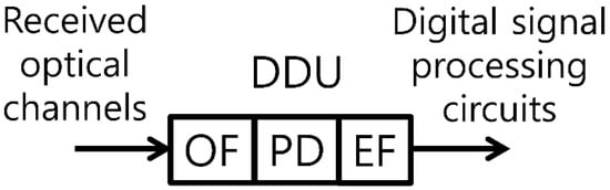
Figure 1. A schematic of DDU that determine the ORM set. OF: optical filter. PD: photodetector. EF: electrical filter.

For this DDU, the ORM integral equation for the n-th ORM (n = 0, 1, 2, …) is as follows [12]:

$${\varphi }_n\left(\omega \right)={\lambda }_n{\int }_{-\infty }^{\infty }d{\omega }^{\prime }K(\omega ,{\omega }^{\prime }){\varphi }_n\left({\omega }^{\prime }\right),$$

(1)

where ${\varphi }_n\left(\omega \right)$ is the n-th order ORM mode function in the optical frequency domain and ${\lambda }_n$ is its eigenvalue. $\omega$ is the angular frequency deviation from the center angular frequency of the received optical channel. The kernel $K\left({\omega ,\omega }^{\prime }\right)$ is given as:

$$K\left({\omega ,\omega }^{\prime }\right)=H_o^{*}\left(\omega \right)H_e({\omega }^{\prime }-\omega )H_o\left({\omega }^{\prime }\right),$$

(2)

where $H_o\left(\omega \right)$ is the transfer function of the OF for the complex electric field amplitude of the received optical channels [7]. The asterisk means the complex conjugation. $H_e\left(\omega \right)$ is the transfer function of the EF for the electrical signal from the PD. Note that $K\left({\omega ,\omega }^{\prime }\right)$ is Hermitian, $K^{*}\left({\omega ,\omega }^{\prime }\right)=K\left({\omega }^{\prime },\omega \right)$. Thus, the eigenvalues are real and the mode functions are complete with the orthogonality relation:

$${\int }_{-\infty }^{\infty }d\omega {{\varphi }_m^{*}\left(\omega \right)\varphi }_n\left(\omega \right)=2\pi {\delta }_{mn},$$

(3)

where ${\delta }_{mn}$ is the Kronecker delta function.

3. Proposed Method

Inserting (2) into (1), we obtain:

$${\varphi }_n\left(\omega \right)={\lambda }_n{\int }_{-\infty }^{\infty }d{\omega }^{\prime }{H}_o^{*}\left(\omega \right)H_e\left({\omega }^{\prime }-\omega \right)H_o\left({\omega }^{\prime }\right){\varphi }_n\left({\omega }^{\prime }\right).$$

(4)

Let us introduce a new function $U_n\left(\omega \right)$ defined by:

$$U_n\left(\omega \right)=H_o\left(\omega \right){\varphi }_n\left(\omega \right).$$

(5)

Then, $U_n\left(\omega \right)$ satisfies the following integral equation from (4):

$$U_n\left(\omega \right)={\lambda }_n|H_o(\omega ){|}^2{\int }_{-\infty }^{\infty }d{\omega }^{\prime }{H}_e\left({\omega }^{\prime }-\omega \right)U_n\left({\omega }^{\prime }\right).$$

(6)

When $\left|H_o\right(\omega ){|}^2$ is Lorentzian, $|H_o\left(\omega \right){|}^2=|H_o{|}^2({{\omega }_{3dB}/2)}^2/\{{\omega }^2+({{\omega }_{3dB}/2)}^2\}$ [18], or

$$|H_o\left(\omega \right){|}^2={\displaystyle \frac{|H_o{|}^2}{1+4(\omega /{{\omega }_{3dB})}^2}},$$

(7)

(6) becomes:

$${\left\{1+4(\omega /{{\omega }_{3dB})}^2\right\}U}_n\left(\omega \right)={\lambda }_n|H_o{|}^2{\int }_{-\infty }^{\infty }d{\omega }^{\prime }{H}_e\left({\omega }^{\prime }-\omega \right)U_n\left({\omega }^{\prime }\right),$$

(8)

where ${\omega }_{3dB}$ is the 3 dB bandwidth of $|H_o\left(\omega \right){|}^2$. Hereafter, we use the notations, $H_o\left(0\right)=H_o$ and $H_e\left(0\right)=H_e$. From the inverse Fourier transform of (8), we find a one-dimensional Schrödinger equation in the time domain:

$$\left[{\displaystyle \frac{d^2}{{dt}^2}} + {\displaystyle \frac{{\omega }_{3dB}^2}{4}}\left\{2\pi {\lambda }_n|H_o{|}^2{h}_e\left(-t\right)-1\right\}\right]u_n(t)=0,$$

(9)

where $u_n\left(t\right)$ and $h_e\left(t\right)$ are given as:

$$u_n\left(t\right)={\displaystyle \frac{1}{2\pi }}{\int }_{-\infty }^{\infty }d\omega U_n\left(\omega \right)\mathrm{e}\mathrm{x}\mathrm{p}\left(j\omega t\right)$$

(10)

$$h_e\left(t\right)={\displaystyle \frac{1}{2\pi }}{\int }_{-\infty }^{\infty }d\omega H_e\left(\omega \right)\mathrm{e}\mathrm{x}\mathrm{p}\left(j\omega t\right).$$

(11)

The potential of the Schrödinger equation, (9), is proportional to $h_e\left(-t\right)$. If we regard (9) as the Schrödinger equation for a particle [19], the particle energy is negative, −${\omega }_{3dB}^2/4$ times a positive constant. Thus, the potential acts as a potential well and the ORM is one of the bound-states of (9). Note that the particle energy is fixed and the potential is proportional to ${\lambda }_n$.

The Lorentzian condition (7) can be satisfied exactly if the OF is a one-pole bandpass filter:

$$H_o\left(\omega \right)=H_o{\displaystyle \frac{1}{1 + 2j\omega /{\omega }_{3dB}}}.$$

(12)

In real systems, we often use an optical FP filter [18] having two optical mirrors as the OF with the transfer function:

$$H_o\left(\omega \right)=H_o{\displaystyle \frac{1-r}{1-r \mathrm{e}\mathrm{x}\mathrm{p}(-j\theta )}},$$

(13)

where $r$ is the mirror reflectivity and $\theta =\theta \left(\omega \right)=2\pi \omega /{\omega }_{fsr}$. ${\omega }_{fsr}$ is $2\pi$ times the free-spectral range. From (13), we have [18]:

$$|H_o\left(\omega \right){|}^2={\displaystyle \frac{|H_o{|}^2}{1 + 4{\left(F/\pi \right)}^2{\mathrm{s}\mathrm{i}\mathrm{n}}^2(\theta /2)}},$$

(14)

where $F=\mathrm{\pi }\sqrt{r}/(1-r)$ is the finesse of the optical FP filter. When $r\approx 1$, (14) becomes Lorentzian. This is because F is large in this case and $|H_o\left(\omega \right){|}^2$ is non-negligible only when ${\mathrm{s}\mathrm{i}\mathrm{n}}^2(\theta /2)$ is small. Thus, we may approximate ${\mathrm{s}\mathrm{i}\mathrm{n}}^2(\theta /2)\approx {\theta }^2/4 + O\left({\theta }^4\right),$ which gives:

$$|H_o\left(\omega \right){|}^2\approx {\displaystyle \frac{|H_o{|}^2}{1 + {\left(F/\pi \right)}^2{\theta }^2}}.$$

(15)

This is just (7) with ${\omega }_{3dB}={\omega }_{fsr}/F$. Note that for a given r, the error in (15) increases as ${\theta }^2$ increases from zero. Thus, higher-order ORMs evaluated from (9) have larger errors, since higher-order ORMs occupy wider spectral ranges. In the limit of $r\to 1$, (13) becomes (12).

After finding $u_n\left(t\right)$ from (9), we obtain from (5):

$${\psi }_n\left(t\right)={\displaystyle \frac{1}{(1-r)H_o}}\left\{u_n\left(t\right)-r{u}_n(t-T_{fsr})\right\},$$

(16)

where $T_{fsr}=2\pi /{\omega }_{fsr}$ and ${\psi }_n\left(t\right)$ is the n-th order ORM mode function in the time domain:

$${\psi }_n\left(t\right)={\displaystyle \frac{1}{2\pi }}{\int }_{-\infty }^{\infty }d\omega {\varphi }_n\left(\omega \right)\mathrm{e}\mathrm{x}\mathrm{p}\left(j\omega t\right).$$

(17)

4. Square-Well Potential

As a first example, we assume $h_e\left(t\right)=h_e$ for 0 < t < $w$ and $h_e\left(t\right)=0$ otherwise. This is the well-known square-well potential. Note that ${H_e=h}_{e}w$ in this case. The bound-state solution of (9) can be written as [19]:

$$u_n\left(t\right)=\left\{\begin{array}{ccc}{C}_1\exp \gamma \left(t + w/2\right),& t<-w& \left(18\right)\\ A\mathrm{c}\mathrm{o}\mathrm{s}\kappa \left(t + w/2\right) + B\mathrm{s}\mathrm{i}\mathrm{n}\kappa \left(t + w/2\right),& -w< t<0& \left(19\right)\\ C_2\exp \left\{-\gamma \left(\mathit{t}+\mathit{w}/2\right)\right\},& 0<t,& \left(20\right)\end{array}\right.$$

where ${\gamma =\omega }_{3dB}/2$ and $\kappa =\gamma \sqrt{2\pi {|H}_o{|}^2{h_e\lambda }_n-1}$. We have omitted the subscript n for $\kappa$, A, B, C₁, and C₂. For ORMs with even n,${\lambda }_n$ satisfies $\mathrm{t}\mathrm{a}\mathrm{n}(\kappa w/2)=\gamma /\kappa$ and B = 0. For ORMs with odd n, ${\lambda }_n$ satisfies $\mathrm{c}\mathrm{o}\mathrm{t}(\kappa w/2)=-\gamma /\kappa$ and A = 0. The coefficients A, B, C₁, and C₂ are determined from the fact that $u_n\left(t\right)$ and its derivative are continuous at t = 0 and −w and the fact that ${\int }_{-\infty }^{\infty }{\psi }_n^2\left(t\right)dt=1$.

We assume that the optical FP filter’s 3 dB bandwidth or ${\omega }_{3dB}/2\pi$ is 100 GHz with $r=0.95$ (F = 61.2). This is similar to [8] where a Gaussian optical filter is used with the 3 dB bandwidth of 100 GHz. Also, as in [8], the 3 dB bandwidth of $H_e\left(\omega \right)$ is chosen as 10 GHz, which is achieved when $w$ is 60.3 ps. The center wavelength of the received optical channel is at 1550 nm.

We also perform a numerical analysis for the ORM integral Equation (1). The integration range in (1) is chosen from −10 ${\omega }_{3 dB}$ to 10 ${\omega }_{3 dB}.$ Equation (13) is used for $H_o\left(\omega \right)$. The Gauss–Legendre numerical integration technique [20] is used with 1200 points, which leads to a Hermitian matrix eigenvalue problem [20]. To find these parameters, we have to run the program multiple times until we find accurate results. It takes about one hour using a personal computer for a single run.

In Figure 2, we plot ${\psi }_n\left(t\right)$ for n = 0, 10, and 20. The ORM mode functions are sinusoidal for the most part. Both of our analyses using the Schrödinger equation and the numerical analysis give almost the same curves. The eigenvalues in both analyses agree within 1%.

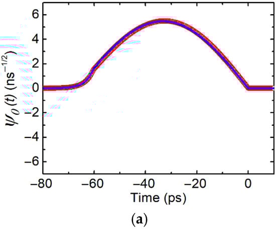
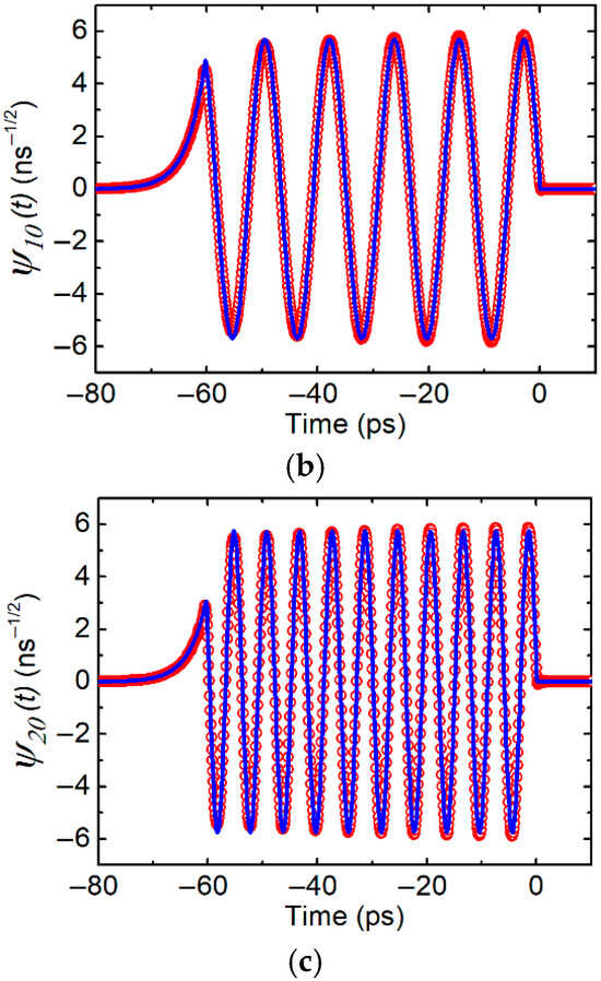
Figure 2. ${\psi }_n\left(t\right)$ for the square-well potential. (a) n = 0, (b) n = 10, and (c) n = 20. The red open circles are results from our analysis using the Schrödinger equation. The blue lines are results from the numerical analysis for the ORM integral equation.

5. Exponential-Well Potential

Next, we assume $h_e\left(t\right)=h_e\mathrm{e}\mathrm{x}\mathrm{p}(-{\omega }_{c}t)$ for 0 < t and $h_e\left(t\right)=0$ otherwise. This corresponds to a single-pole low-pass filter with $H_e\left(\omega \right)=H_e/(1 + j\omega /{\omega }_c)$, where ${\omega }_c/2\pi$ is the cutoff frequency and $H_e=h_e/{\omega }_c$. The Schrödinger equation for the exponential-well potential can be solved exactly using the Bessel function [21,22]. With $x=a \exp \left(bt\right)$, the Bessel function $J_{\mathrm{\nu }}\left(x\right)$ satisfies:

$$\left\{{\displaystyle \frac{d^2}{{dt}^2}} + a^2{b}^2\exp \left(2bt\right)-{\nu }^2{b}^2\right\}{J}_{\nu }\left(x\right)=0,$$

(21)

where a and b are constants. Comparing (21) with (9), we find:

$${ u}_n\left(t\right)=\left\{\begin{array}{ccc}A{J}_{\nu }\left\{a\mathrm{e}\mathrm{x}\mathrm{p}({\omega }_{c}t/2)\right\},& t<0& \left(22\right)\\ B\mathrm{e}\mathrm{x}\mathrm{p}(-{\omega }_{3dB}t/2),& 0\le t,& \left(23\right)\end{array}\right.$$

where ${\nu =\omega }_{3dB}/{\omega }_c$, $a=\nu \sqrt{2\pi {\lambda }_n|H_o{|}^2{h}_e}$, and ${b=\omega }_c/2$. A and B are constants to be determined from the fact that $u_n\left(t\right)$ and its derivative are continuous at $t=0$ and the fact that ${\int }_{-\infty }^{\infty }{\psi }_n^2\left(t\right)dt=1$. Using the continuity condition of $u_n\left(t\right)$ and its derivative at $t=0$, we have $\mathrm{A}{J}_{\nu }\left(a\right)=B$ and $ab\left\{J_{\nu + 1}\left(a\right)-J_{\nu -1}\left(a\right)\right\}={\omega }_{3dB}{J}_{\nu }\left(a\right)$, where we have used the recurrence equation ${2d{J}_{\nu }\left(x\right)/dx=J}_{\nu -1}\left(x\right)-J_{\nu + 1}\left(x\right)$.

As in the square-well potential case, the optical FP filter’s 3 dB bandwidth is 100 GHz with $r=0.95$ (F = 61.2). The cutoff frequency of the EF is 10 GHz. Thus, we have ν = 10. We use the following expression to evaluate the Bessel function having an integer order of m:

$$J_m\left(x\right)={\displaystyle \frac{1}{\pi }}{\int }_0^{\pi }\cos \left(m\theta -x\mathrm{s}\mathrm{i}\mathrm{n}\theta \right)d\theta .$$

(24)

The numerical analysis of the ORM integral Equation (1) is also performed in the same way as the square-well potential case. In Figure 3, we plot ${\psi }_n\left(t\right)$ for n = 0, 10, and 30. The exponential-well potential case also gives sinusoidal ORM mode functions but with chirping. Both our analyses using the Schrödinger equation and the numerical analysis give almost the same curves. The eigenvalues in both analyses also agree within 1%.

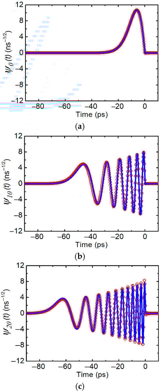
Figure 3. ${\psi }_n\left(t\right)$ for the exponential-well potential. (a) n = 0, (b) n = 10, and (c) n = 20. The red open circles are results from our analysis using the Schrödinger equation. The blue lines are results from the numerical analysis for the ORM integral equation.

6. Discussion

The Schrödinger equation has been also used to analyze optical slab waveguides [21,22]. The Schrödinger equation can be solved exactly for various potential cases. Even if there are no analytical solutions available, the numerical analysis for the Schrödinger equation can be conducted very quickly and accurately by approximating the potential as a piecewise linear function [23] or a piecewise parabolic function [24].

The two potentials presented here provide closed-form solutions. Although the $h_e\left(t\right)$ in the actual system may be different from our examples, we may guess roughly the behavior of solutions from the solutions presented here, which will be very helpful.

If the finesse F is too low, the validity of using the Schrödinger equation is weakened. It depends on the spectral range of the ORM mode functions. For example, if the error in ${\lambda }_{20}$ needs to be less than 2%, the Schrödinger Equation (9) can be used for F greater than 20 (r = 0.855) for the square-well potential case and greater than 30 (r = 0.901) for the exponential-well potential case. The difference in F values here results from the spectral range of ${\psi }_{20}\left(t\right)$ being wider in the exponential-well potential case. For lower-order modes, their spectral ranges are narrower than that of ${\psi }_{20}\left(t\right)$. Thus, their eigenvalues have errors less than that of ${\lambda }_{20}$ for the same F.

The ORM integral equation belongs to the homogeneous Fredholm equation of the second kind [25], which cannot be transformed into a differential equation in general. One of the interesting points of this paper is that the ORM integral equation can be transformed into a differential equation when the OF is an optical FP filter.

In our two examples, the square-well potential and the exponential-well potential cases, $h_e\left(t\right)$ is non-negative for all t. Thus, from (9), we can see that ${\lambda }_n$ is positive and increases indefinitely as n increases [9,12]. Since the electrical signals generated by the n-th ORM are proportional to 1/${\lambda }_n$ for both DD optical receivers [5] and CO receivers [7], it is important to reduce the increase rate of ${\lambda }_n$ to use as many ORMs as possible. This can be achieved by decreasing the bandwidth of the EF with the ${\omega }_{3dB}$ fixed. Then, $h_e\left(t\right)$ becomes broader and the bound state energies become closer. This is why the 3 dB bandwidth of the EF is chosen as 1/10 of ${\omega }_{3dB}/2\pi ,$ as in [8].

As n increases, ${\lambda }_n$ increases more steeply in the exponential-well potential case than in the square-well potential case. For example, the eigenvalue ratios are 3.85 for ${\lambda }_{10}/{\lambda }_0$ and 11.9 for ${\lambda }_{20}/{\lambda }_0$ in the square-well potential case. In the exponential-well potential case, the ratios of the eigenvalues are 12.4 for ${\lambda }_{10}/{\lambda }_0$ and 34.8 for ${\lambda }_{20}/{\lambda }_0$. All these ratios are evaluated from our analysis using the Schrödinger equation. Therefore, it may be necessary to reduce the bandwidth of the EF further in the exponential-well potential case to increase the SE. This will also reduce high-frequency components in the exponential-well potential case owing to the chirping in the ORM mode functions.

For future works, it will be interesting to find other differential equations equivalent to the ORM integral equation when the OF is not Lorentzian.

7. Conclusions

To find the mode functions and the eigenvalues of ORMs when the OF is the optical FP filter, we have introduced a new method that uses the Schrödinger equation instead of solving the ORM integral equation numerically. Our method provides a substantially faster way to evaluate the mode functions and eigenvalues of ORMs than numerically solving the ORM integral equation. The Schrödinger equation has exact solutions for a variety of potentials. When no analytical solutions are available, numerical analysis can be conducted very quickly and accurately by approximating the potential with a piecewise linear function [23] or a piecewise parabolic function [24]. Using this method, we have evaluated the mode functions and the eigenvalues of ORMs for two potential cases that have exact solutions. One is the square-well potential case and the other is the exponential-well potential case.

References

- Essiambre, R.J.; Kramer, G.; Winzer, P.J.; Foschini, G.J.; Goebel, B. Capacity limits of optical fiber networks. J. Light. Technol. 2010, 28, 662–701. [Google Scholar] [CrossRef]
- Puttnam, B.J.; Luís, R.S.; Rademacher, G.; Mendez-Astudillio, M.; Awaji, Y.; Furukawa, H. S-, C- and L-band transmission over a 157 nm bandwidth using doped fiber and distributed Raman amplification. Opt. Express 2022, 39, 10011–10018. [Google Scholar] [CrossRef] [PubMed]
- Klaus, W.; Winzer, P.J.; Nakajima, K. The role of parallelism in the evolution of optical fiber communication systems. Proc. IEEE 2022, 110, 1619–1654. [Google Scholar] [CrossRef]
- Agrell, E.; Karlsson, M.; Poletti, F.; Namiki, S.; Chen, X.; Rusch, L.A.; Puttnam, B.J.; Bayvel, P.; Schmalen, L.; Tao, Z.; et al. Roadmap on optical communications. J. Opt. 2024, 26, 093001. [Google Scholar] [CrossRef]
- Lee, J.S. Optical signals using superposition of optical receiver modes. Curr. Opt. Photonics 2017, 1, 308–314. [Google Scholar]
- Batsuren, B.; Seo, K.H.; Lee, J.S. Optical communication using linear sums of optical receiver modes: Proof of concept. IEEE Photonics Technol. Lett. 2018, 30, 1707–1710. [Google Scholar] [CrossRef]
- Lee, J.S. Coherent optical receiver for real-time CO-ORMDM systems. Curr. Opt. Photonics 2023, 7, 15–20. [Google Scholar]
- Seo, K.H.; Lee, J.S. Method of crosstalk analysis for CO-ORMDM systems. Curr. Opt. Photonics 2024, 8, 156–161. [Google Scholar]
- Lee, J.S.; Shim, C.S. Bit-error-rate analysis of optically preamplified receivers using an eigenfunction expansion method in optical frequency domain. J. Light. Technol. 1994, 12, 1224–1229. [Google Scholar]
- Forestieri, E. Evaluating the error probability in lightwave systems with chromatic dispersion, arbitrary pulse shape and pre- and postdetection filtering. J. Light. Technol. 2000, 18, 1493–1503. [Google Scholar] [CrossRef]
- Holzlohner, R.; Grigoryan, V.S.; Menyuk, C.R.; Kath, W.L. Accurate calculation of eye diagrams and bit error rates in optical transmission systems using linearization. J. Light. Technol. 2002, 20, 389–400. [Google Scholar] [CrossRef]
- Lee, J.S.; Willner, A.E. Analysis of Gaussian optical receivers. J. Light. Technol. 2013, 31, 2687–2693. [Google Scholar] [CrossRef]
- Djordjevic, I.B.; Vasic, B. Orthogonal frequency division multiplexing for high-speed optical transmission. Opt. Express 2006, 14, 3767–3775. [Google Scholar] [CrossRef] [PubMed]
- Qian, D.; Huang, M.-F.; Ip, E.; Huang, Y.-K.; Shao, Y.; Hu, J.; Wang, T. 101.7-Tb/s (370×294-Gb/s) PDM-128QAM-OFDM transmission over 3×55-km SSMF using pilot-based phase noise mitigation. In Proceedings of the Optical Fiber Communication Conference, Los Angelis, CA, USA, 6–10 March 2011; Optica Publishing Group: Washington, DC, USA, 2011; p. PDPB5. [Google Scholar]
- Omiya, T.; Yoshida, M.; Nakazawa, M. 400 Gbit/s 256 QAM-OFDM transmission over 720 km with a 14 bit/s/Hz spectral efficiency by using high-resolution FDE. Opt. Express 2013, 21, 2632–2641. [Google Scholar] [CrossRef] [PubMed]
- Kikuchi, K. Fundamentals of coherent optical fiber communications. J. Light. Technol. 2016, 34, 157–179. [Google Scholar] [CrossRef]
- Winzer, P.J. High-spectral-efficiency optical modulation formats. J. Light. Technol. 2012, 30, 3824–3835. [Google Scholar] [CrossRef]
- Saleh, B.E.A.; Teich, M.C. Fundamentals of Photonics; Wiley: New York, NY, USA, 1991; pp. 316–320. [Google Scholar]
- Gasiorowicz, S. Quantum Physics; John Wiley & Sons: New York, NY, USA, 1974; pp. 45–109. [Google Scholar]
- Press, W.H.; Flannery, B.P.; Teukolsky, S.A.; Vetterling, W.T. Numerical Recipes; Cambridge University Press: New York, NY, USA, 1986; pp. 121–126. [Google Scholar]
- Conwell, E.M. Modes in optical waveguides formed by diffusion. Appl. Phys. Lett. 1973, 23, 328–329. [Google Scholar] [CrossRef]
- Kogelnik, H. Theory of dielectric waveguides. In Integrated Optics; Tamir, T., Ed.; Springer: Berlin, Germany, 1975; pp. 13–81. [Google Scholar]
- Lui, W.W.; Fukuma, M. Exact solution of the Schrödinger equation across an arbitrary one-dimensional piecewise-linear potential barrier. J. Appl. Phys. 1986, 60, 1555–1559. [Google Scholar] [CrossRef]
- Neufeld, O.; Sharabi, Y.; Ben-Asher, A.; Moiseyev, N. Calculating bound states resonances and scattering amplitudes for arbitrary 1D potentials with piecewise parabolas. J. Phys. A Math. Theor. 2018, 51, 475301. [Google Scholar] [CrossRef]
- Arfken, G.B.; Weber, H.J.; Harris, F.E. Mathematical Methods for Physicists, 7th ed.; Elsevier Academic: New York, NY, USA, 2013; pp. 1047–1079. [Google Scholar]
Disclaimer/Publisher’s Note: The statements, opinions and data contained in all publications are solely those of the individual author(s) and contributor(s) and not of MDPI and/or the editor(s). MDPI and/or the editor(s) disclaim responsibility for any injury to people or property resulting from any ideas, methods, instructions or products referred to in the content. |
© 2025 by the authors. Licensee MDPI, Basel, Switzerland. This article is an open access article distributed under the terms and conditions of the Creative Commons Attribution (CC BY) license.