Experimental and Theoretical Research on Pressure Drop Changes in a Two-Stage Air Filter Used in Tracked Vehicle Engine

Abstract

The effect of mineral dust in the air sucked in by an engine on accelerated component wear and reduction in performance was presented. The necessity to use two-stage air filters (multicyclone-paper insert) for military vehicles was shown. The results showed that placing an air filter in the path of the air entering the engine causes an additional pressure drop (air filter resistance increase), which leads to engine power decrease and increased fuel consumption. An analysis of model filter beds’ pressure drop changes (depending on bed parameters, aerosol flow parameters, and dust content) was carried out. It was revealed that it is very difficult to model changes in pressure drop in filter beds for actual conditions that appear during vehicle operation. The air filter pressure drop measurement results of more than 20 tracked vehicles operating in variable air dust concentration conditions were presented. The forms of selected regression models of the “life curve” type, best suited to the actual changes in air filters pressure drop as a function of the vehicle mileage, were determined. Significant differences were found between the same model values for different units of the tested vehicles. The quality of forecasting pressure drop value by selected functions was assessed by extrapolating them to the value of the next measurement and comparing the forecast and actual value. It was found that for the performed experiment, sufficiently good results of experimental data approximation and forecasting were obtained for a simple linear model.

1. Introduction

Military motor vehicles and working machines are mainly operated off-road, in sandy and desert terrain, where mineral dust concentration in the air is particularly high and often exceeds 1 g/m³. This is very important for trucks and special vehicles, whose power units are high-power diesel engines with large (1000–6000 m³/h) volumetric air demand. A PT-91 tank engine travelling at a velocity of 20 km/h on military training area roads, where concentration of dust suspended in the air is 1 g/m³, sucks in more than 170 kg dust with the air within 1000 km (approximately 50 h of operation). Thus, the air filters are of large-size, heavy, time-consuming, and costly to maintain.

A common air pollutant sucked in by motor vehicle engines is mineral dust (road dust) carried from the area by moving vehicles or by wind. Basic road dust components constitute SiO₂ silica and Al₂O₃ corundum, whose dust share reaches 95%; and Fe₂O₃, MgO, and CaO. Furthermore, the dust consists of K₂O, Na₂O, and SO₃ [1,2]. The physico-chemical dust composition strictly depends on the composition and type of substrate, climatic factors (winds, rains, snow, frost, droughts, etc.), and sedimentation of industrial dust, and dust from forest fires and volcanic ash [3].

Road dust, like most naturally occurring dusts, is polydisperse. Dust grains with a diameter of d_p < 2 µm remain in the air for a very long time (their mass share in the total amount of dust is usually small). Dust grains with d_p = 2–10 µm stay in the air for a long time and are sucked in by the engines. Dust grains with d_p = 10–50 µm constitute a significant share in the total air mass sucked in by the engine when the vehicle is operated in conditions of high dust concentration in the air. Dust grains larger than 50 µm are found in the air in training yards, military training areas, quarries, construction sites, and mines [4].

Dust concentration in the air around a moving vehicle is variable and depends on the type of area, traffic, vehicle movement conditions, meteorological conditions, aerodynamic properties of the vehicle, type of wheels and steering system, type of surrounding soils, and height.

Typical concentrations can range from 0.01 mg/m³ in clean rural environments and up to about 20 g/m³ in heavy desert vehicle convoys [5,6]. According to [7], dust concentration in dusty environments is in the range of 0.001–10 g/m³. The authors of [8] investigated that the maximum dustiness within a few meters from all-terrain vehicles driving on a sandy road is 0.05–10 g/m³. The authors of [9] state that the dust concentration on highways ranges from 0.0004–0.1 g/m³ to 0.03–8 g/m³ when a column of vehicles is moving on sandy terrain. Similar dust concentration values in the air occur during take-off or landing of a helicopter at an accidental landing site. The rotating propeller lifts large amounts of mineral dust from the ground, which the engine absorbs with the air. The highest dust concentration values are found low (0.5 m) above the ground. At the height of the propeller end of the CH-53 helicopter taking off, the dust concentration may have the value s = 3.33 g/m³, and at a distance of 30 m, s = 2.11 g/m³ [10]. However, the actual dust concentration at the inlet to the engine intake system does not often exceed the value of 2.5 g/m³ [5,7,8]. Dust air concentration within the limits of 0.6–0.7 g/m³ significantly reduces visibility, and at a concentration of about 1.5 g/m³, it is practically zero [11].

Dust suspended in the air is highly abrasive and is the most common cause of accelerated wear of two frictionally matching parts, such as the P-PR-CW engine components (piston-piston rings-cylinder walls). According to the hardness on the basis of the ten-level Mohs scale, where 10 corresponds to diamond hardness, silica has a hardness of 7, and corundum of 9. Dust sucked in with the air goes over the piston and the aforementioned constitutes a decisive factor that the upper part of the cylinder and piston and the upper piston rings wear the most. Abrasive engine component wear is caused mainly by particles of 1–40 µm, with the most harmful particles occurring within the range of 1–20 µm [2,7,10,12]. The authors of [12] state that approximately 30% of pollutants entering the engine may be released, essentially in the unchanged form, along with exhaust gases from the cylinders to the exhaust system, thus increasing the emission of particulate matter (PM) from the engine. Only 10–20% of the dust enters the engine with the air through the intake system sediments on cylinder liner walls. Together with the oil, this dust part forms a kind of the abrasive paste which, in contact with engine mating surfaces, for example P-PR-CW, causes abrasive wear. The remaining part of the dust is evaporated or oxidised during the fuel combustion process in the cylinder (under high pressure and high temperature conditions).

Some mineral dust particles, the melting point of which is much lower than the peak temperature in the combustion chamber (2000–2500 °C), melt and then, along with the exhaust gases, enter the exhaust system and sediment on the cooler surfaces with which they come into contact (for example, in a catalytic converter) forming a glassy surface. This results from the fact that each of the polymorphic forms of SiO₂ quartz (tridymite and cristobalite) is stable in the appropriate temperature range. At 1600 °C, the quartz melts to give quartz glass [13].

The most dangerous for the two working components are dust particles featuring a diameter d_p equal to the oil film thickness h_min between two surfaces at a concerned moment. In typical combustion engine combinations, oil film thicknesses vary within the range of h_min = 0.3–10 µm [14].

The excessive wear of P-PR-CW causes increased blow-by of fresh load into the crankcase, resulting in compression pressure and engine power drop [15], increased oil aging, and increased oil flowing consumption over the piston, which increases solid particles emission [16,17,18]. One way to reduce friction and wear of the P-PR-CW connection is to apply a chromium nitride coating to the cylinder liner surface [19].

Adequate air purity at the inlet to traction motors is ensured by air filters, which differ in their principle and mode of operation, design, separation partition type, and operating efficiency. Trucks, special vehicles (tanks, armoured personnel carriers, infantry fighting vehicles), and working machines engines operating in high dust concentrations conditions in air are equipped with two-stage filters.

The idea of using two-stage filters is to pre-separate in an inertial filter (multicyclone, monocyclone) dust grains of the largest size and mass (d_p > 15–35 µm). Then, small-sized dust grains remain in the air stream, which are directed to the filter cartridge, usually made of pleated paper with a suitably selected surface, where they are retained with an accuracy of greater than d_p = 2–5 µm. As a result, air is supplied to the engine cylinders with the required purity and filtration system operation time is extended; thus, the service interval is limited by reaching a certain value of the pressure drop determined for a given engine for the permissible pressure drop Δp_fdop.

The first filtration stage is then an inertial multi-cyclone filter, and the second a porous barrier in the form of a cylindrical pleated paper insert, which is the dominant material that filters air sucked in by internal combustion engines. 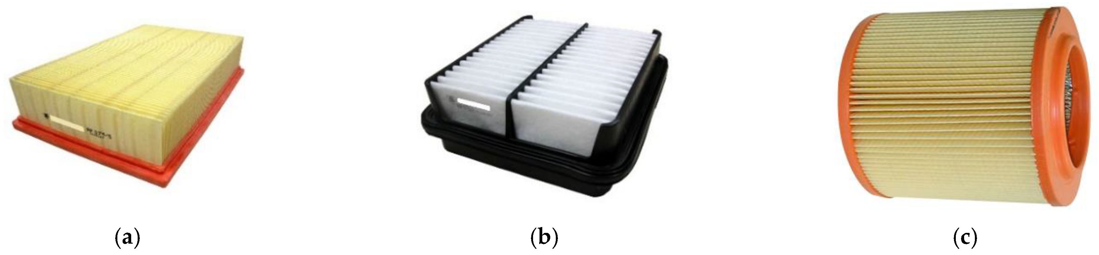Filter papers are characterized by high efficiency (over 99.5%) and accuracy—over 5 µm, but low water absorption (in the range of 200–250 g/m²), which forces designers to construct filters with a large paper surface [12,20,21]. Modern air filters use filter cartridges made of filter paper or pleated nonwoven fabric (Figure 1), due to the fact that the largest possible surface of the paper is obtained in a limited space in the engine compartment.

Non-woven materials and metal mesh are also used to filter engine intake air. In many military vehicles, which are operated in high dust concentration conditions in air, irregular, oil-soaked filter beds made of thin metal wire are still used as second filtration [22]. Plastic filter materials soaked in oil are still used in many agricultural tractors. Since the early 1990s, it has been popular in most Asian countries to further improve filtration efficiency and to lubricate pleated disposable filter elements for intake air in motor vehicles [23]. It has been proven that such a procedure ensures greater efficiency and dust absorption as well as sufficiently long service intervals. In addition, the oil is both chemically stable and harmless to the engine itself, and suppresses solid particles re-entrainment. It was found that oil coating on flat fibrous filters resulted in increased dust holding capacity, reduced pressure drop over time and reduced efficiency at lower filtration speeds. The authors of [23,24] reported that flat fiber filters’ filtration efficiency is largely affected by the amount of oil. It was found that higher amounts of oil resulted in higher particle filtration efficiency, but at the cost of a higher pressure drop, which is not desired.

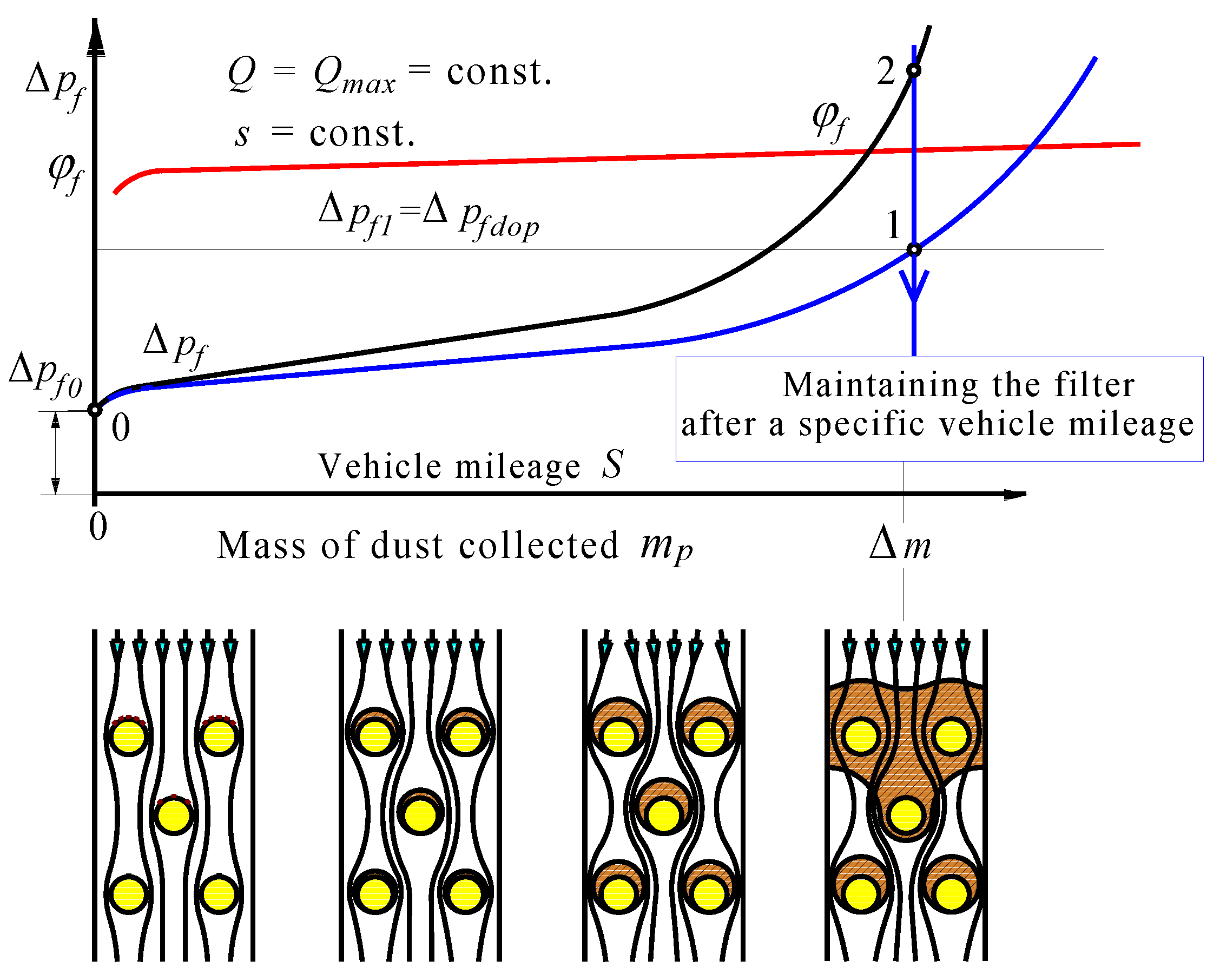
During engine operation, as a result of the deposition and accumulation of dust particles on the filter cartridge, filter pressure drop Δp_f increases (Figure 2). The intensity of filter pressure drop increase depends on the conditions in which the vehicle is operated, mainly on dust concentration in air and vehicle (engine) operating time. Excessively contaminated air filter elements cause difficult air flow to the engine, which reduces engine cylinders from filling [25,26]. This directly affects conditions of fuel combustion process, which may deteriorate engine performance (power decrease and fuel consumption increase) or cause an unfavorable change in exhaust gas composition [27,28]. Therefore, manufacturers, depending on the engine type, set permissible pressure drop value Δp_fdop, which should not be exceeded by the air filter while the vehicle is in use. For high power diesel engines, these values are in the range of 3.7–7.5 kPa [26]. For SI engines, Δp_fdop values are within the range of 3.8–5 kPa [29], while in [30], it was stated that maximum pressure drop values limiting the air supply for diesel engines with a turbocharger usually assume values of 5–7, 6 kPa. For special vehicles engines, the admissible pressure drop values are in the range of 9–12 kPa [31]. From a technical point of view, air filter service life is commonly defined as the restriction level, which causes pressure drop in passenger car filter by about 2.5 kPa above the pressure drop of new (clean) filter [32]. For trucks and special vehicles, it is assumed that Δp_fdop values are approximately 6.25–7.5 kPa above pressure drop of the clean air filter [33].

Truck and special vehicles driving units are self-ignition engines of high power and large (1000–6000 m³/h) volumetric air demand. Thus, air filters are large, heavy, time-consuming, and costly to maintain. These vehicles are operated in conditions of high and variable air pollutants concentrations, and thus pressure drop increase varies with intensity. Therefore, servicing the filter (performed after specified vehicle mileage standard) may be premature, which increases operating costs, or too late. In the second case, the increase in the filter pressure drop caused by the continuous accumulation of dust on the air filter element and resulting from the high dust concentration in the air, is more intense, which results in exceeding the set value of Δp_fdop (Figure 1). 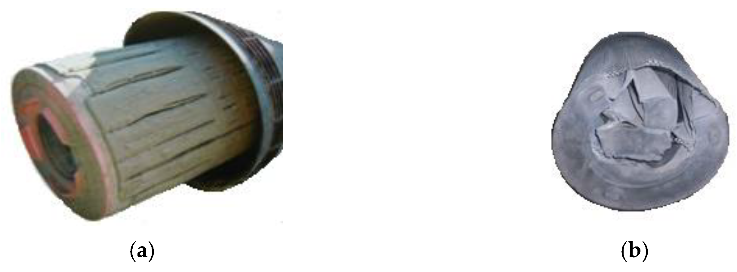Further operation of the filter is possible, but the rapidly increasing pressure drop causes an additional engine power decrease and a fuel consumption increase [33,34,35]. Moreover, the high negative pressure behind the filter and vibrations of the filter element caused by cyclically sucked air pulsations may also cause mechanical filter element destruction (Figure 3).

Pressure drop increase in the compression ignition engine inlet system by 1 kPa causes an average engine power decrease by 0.4–0.6% and fuel consumption increase by about 0.3–0.5% [4].

The challenge for scientists is not only to achieve a lower pressure drop and a longer filter life while removing particles with maximum efficiency, but also to know and then predict changes in the air filter pressure drop, depending on vehicle mileage operating in conditions of high and variable dust concentrations, which will allow servicing of the air filter to be performed once Δp_fdop is reached.

The most reliable research method in this area are experimental tests in real operating conditions with the possibility of ongoing filter pressure drop registration. The high cost and difficulties of conducting such research are obvious. For this reason, and due to the large number of parameters determining air filter flow efficiency and resistance, as well as large computers computing capabilities, numerical tests in the form of CFD programs are widely used. Numerical testing eliminates the need for time-consuming and costly experiments during the cycle. For air filters, it is possible to forecast changes in flow resistance, depending on the vehicle mileage.

2. Literature Review in the Field of Research Changes in Filter Materials Pressure Drop

Forecasting is now recognized as a key feature of machinery and equipment operating strategies, giving operators an important decision-making tool by quantifying the amount of time remaining until functionality is lost. The remaining machinery service life can be estimated using the four main condition forecasting techniques. These are experience-driven, model-driven, data-driven, and hybrid activities. Experience-based (or reliability-based) actions use data and knowledge gained during the machine’s past service life. Forecasting is used comprehensively, for example to forecast pollutants in the atmosphere, and in particular PM 2.5 concentration, as an effective way to help in management of measures important for air quality [36,37]; forecasting monthly water streams flow for effective planning and water resources management [38]; forecasting rain-fed agricultural production in dry and semi-dry areas [39]; end point of soot filtration process in diesel particulate filters for diesel engines, using for this purpose changes in pressure drop caused by soot accumulation [40]; long-term electric vehicles charging load [41]; engine oil level using artificial neural networks, which can help classify the state of oil degradation with high accuracy and plan replacement time [42]; frequency of changing the tractor engine oil based on the properties and oil concentration of contaminants [43], which will help to prevent engine failures and time at the charging station for each individual charging process of electric vehicle batteries [44]; heat demand for individual buildings, which should enable demand management and lead to predictive optimization of heat demand at the city level [45].

In the available literature, it is hard to find materials describing research on forecasting air filter pressure drop changes, despite the importance of the task it has in protecting the engine against premature wear.

There is, however, a significant number of works presenting the results of air filters optimization in the direction of flow resistance minimizing and maintaining high filtration efficiency at the same time. This direction of research is caused by the continuous technological development of car engines, which are equipped with newer systems and devices, as a result of which the space available for the air filter is reduced. As a result, the filtration surface is reduced and the filtration speed increases. For filter paper used in car air filters, the maximum filtration speed should not exceed the permissible value (0.08–0.12 m/s) [20,46]. Exceeding this value may result in filtration efficiency decrease due to the phenomenon of reflection and particles re-entrainment [47]. The basic method of ensuring the required surface of the filter material is its pleating.

The quantity, height, and pleats width are the main filter cartridge dimensions that describe the pleating geometry and determine filtration paper surface area. They also have a significant influence on the flow field, both in respect of the air and dust particles, through and near the pleated surface of the filter material, which in turn affects the separation efficiency and pressure drop.

Pleated fibrous material separation efficiency and pressure drop of the intake air filters in vehicle engines have been researched by several researchers, both in numerical and experimental terms. It has been evidenced that each clean pleated filter made from the pleated material has been characterised by an optimal quantity of the pleats, with which it has shown the minimum pressure drop [48,49,50]. Within a course of the researches performed without dust presence, it has been determined that the pressure drop has initially decreased as the quantity of the pleats has grown and then it has increased.

Chen et al. [51] conducted a simultaneous pressure drop and separation efficiency optimisation by means of the pleat quality factor. They found that a value of the pleat quality factor q_p initially increased as the quantity of the pleats has grown, and then decreased. The quality factor of the pleat q_p was defined as the quotient of pleat height (vertical distance from the upper edge of the pleat to the base) and its spacing (the distance between pleat tops). Théron et al. [52] numerically and experimentally evaluated pleat geometrical characteristics influence on pleated fibrous filters performances in the depth filtration stage of sub-micronic aerosols. Wiegmann et al. [53] simulated the pleated air filter with different pleat shapes and filter media and their impact on the pressure drop. This paper [48] experimentally and numerically investigated the pleated air filter with different parameters leading to improve engine performance. A series of parameters were investigated including: pleat height, pleat spacing, pleat shape, filter medium thickness, air velocity, engine speed, and engine torque. The findings showed that lower pressure drop was obtained at the sine wave-shaped pleated air filter. Mahesh [54] numerically investigated the pressure drop characteristics of the air filter of a four-cylinder engine with a triangular and rectangular element.

Several researches have also been carried out to assess the separation efficiency of the pleated fibrous filters with dust presence. Rebai et al. [55] determined that the optimum quantity of the pleats resulting from the researches on filter pressure drop in clean state was significantly lower than the pressure drop based on dust mass captured in the filter. Fotovati et al. [56] researched pleated bed geometry influence on dust deposition in the pleats, as well as on the related pressure drop and separation efficiency. The latter conducted numerical researches maintaining a constant pleat height. Feng and Long [57] developed a CFD simulation on a macroscale to research an optimal design of the pleated air filter under dust loading conditions. It was found that optimum pleated density in the clean state can lead to a higher energy consumption during the dusting process. As has been observed, an optimal dust deposition resulting from pleats density depends on pleat height and is lower when the pleat height is greater.

Saleh and Tafreshi [58] numerically developed a pleated air filter with rectangular and triangular pleats in both depth and surface filtration regimes under dust loading. Pressure drop and filtration efficiency were examined too. To determine the flow field, numerical simulations were carried out on a pleated panel-type air filter with a pleat height of 26 mm, a pleat spacing of 4.5 mm, and a pleat angle of 2.5 degrees. A series of ISO 12103 A2 fine dust tests were carried out on flat cellulose filter material with different speeds in the range of 0.05–0.35 m/s [59,60], experimentally studied pleat geometry effects, and dust load on the pressure drop. The results indicated that the efficient filtration area was mainly influenced by the pleat ratio, so it should be kept below q_p = 1.59.

Numerical models can also be used to forecast changes in filtration efficiency and filter pressure drop during operation. Available literature contains studies where models for predicting filter pressure drop were made for a specific project and relate to samples of filter material, filter cartridges sections, complete single-stage, and two-stage filters.

Paper [61] presents a numerical methodology related to pressure drop in an air filter with a pleated filter component prediction. Pleat geometry and inlet velocity have been determined to be the key optimisation parameters for the filter components. Optimal pleats pitch has been determined to obtain a minimum pressure drop and found to be highly dependent on pleat height. Nevertheless, the authors of [62] used a dimensionless semi-empirical model for the purposes of pleat geometry optimisation, based on vehicle filters experimental and numerical tests results. It was determined that for a given pleat height and a constant air stream, there is such a width between the pleats for which the pressure drop reaches the smallest value. Pressure drop [63] and separation efficiency in a filter featuring the triangular and rectangular pleats have been modelled depending on a number of parameters, including, inter alia, pleat geometry, flow properties, fibre diameter, filter porosity, and particle inertia. Advantage of the algebraic expressions developed in the paper is that they are easy to use when designing a pleated filter and can be used in the initial design stage.

The predictive model related to the characteristics of the non-woven filters [64] takes into account filter parameters (bed thickness, packing density, fibre diameter), operating conditions (separation velocity, temperature), and pollutants in nanoparticle form with sizes ranging between 0–700 nm. Numerical and laboratory tests at separation velocity υ_F = 0.038 m/s and, depending on dust mass deposited on the filter surface, within the range of 0–3 g/m² have been conducted. Filter papers used in the vehicle filters achieve a dust load of 220–250 g/m². There is no information in the paper on the possibility of using this model to predict fibrous bed pressure drop with coarse-grained dust, with a grain size considerably above 1 µm, as it is the case with air filters used in trucks and special vehicles. The possibility of considering dust when modelling the pressure drop for a PTFE polytetrafluoroethylene membrane and HEPA filters is presented in the paper [65]. Model test results have been verified experimentally. In an experiment in respect of dust loading on the PTFE, HEPA membranes were conducted with monodisperse SiO₂ dust with regard to the various particle diameters ranging between 52–553 nm and polydisperse SiO₂ dust. Experimental researches have evidenced that an intensity in pressure drop increase is greater with smaller particle diameter. The aforementioned is consistent with research results [66,67]. Furthermore, the smaller the particle diameter, the greater the efficiency obtained. Developed models can be applied to entire fibrous filter materials filtration process with polydisperse dust. The model presented in [68] was developed in order to predict efficiency and filter pressure drop, depending on the porosity and filter bed thickness as well as fibre diameter, and has included dust particles ranging between 0.1–1 µm. Model tests were carried out for various porosity filter (from 50% to 90%) and thickness: 8, 16, 32, 64, 128, and 512 µm. An equation that fits the pressure drop changes exponentially with the porosity and fibre diameter for the same filter bed thickness was developed. It has been determined that this equation can be used to predict the pressure drop at the filter.

Pressure drop [69] in filters with an additional layer of nanofibers applied to a standard filter bed was forecasted, depending on average fiber diameter (61–260 nm), thickness (0.33–2.17 μm), and filter bed packing density. It has been found that a pressure drop is proportional to the inlet velocity and filter thickness. Such inlet velocity values occur in passenger cars and trucks filter beds, which makes it possible to use results to predict the pressure drop in these filters. Regrettably, the model fails to predict the pressure drop depending on the dust load.

A two-layer filter [12] material made from microfibers and sub-microfibers was developed for use in vehicle engines air filters. Laboratory research of the composite in respect of the separation velocity υ_F = 0.11 m/s with fine-grained test dust (ISO 12103-1) with a concentration of 1 mg/m³ was conducted. The results were compared with the research results of other filter materials. When the pressure drop of the standard medium reached 2 kPa with a dust load of 64 g/m², the pressure drop of the composite for the same dust mass was 38% lower than for the standard medium, featuring high strength. Test results of two trucks in a sandy terrain with high dustiness confirmed lower (about 45%) filter pressure drop with composite material than the filter with standard material.

Numerical and experimental researches [70] were conducted on two filter samples made from nanofibers (d_w = 187 nm, d_w = 283 nm) and microfibers (d_w = 2.7 µm), respectively. Samples arranged individually as composites of two samples adjacent to each other and a kit of two samples positioned at a certain distance were subject to the research. Researches carried out with the use of sodium chloride particles with a size within the range of 40–500 nm evidenced a diversified, in terms of mileage and value, increase in samples pressure drop depending on their configuration.

As particle deposition on microfiber sample (M) increases, there is a slow exponential increase in the pressure drop until a linear trend is reached, the slope of which is the same as the total decrease in linear trend pressure in both samples (M) and (N).

Comparative tests [23] were carried out on standard dry filter papers and the same filter beds containing different oil amounts, corresponding to 0%, 40%, and 80% of dry filter weight. Pressure drop and flow resistance tests on filter paper with a thickness of about 0.6 mm and a grammage of 102 g/m² were performed using fine dust at constant filtration speeds between 0.11 m/s, 0.17 m/s, 0.33 m/s. In the case of media without oil, pressure drop increases rapidly from the very beginning, while in the case of media with oil, the increase intensity is low over a long period of dust accumulation.

The presented analysis shows that filter materials pressure drop depends and can be modeled with high accuracy depending on filter material parameters, which significantly simplifies the process of designing air filters. In real operating conditions, pressure drop depends mainly on dust mass retained on the filter bed and the aerosol flow conditions. The conducted analysis showed that it is possible to model the flow resistance with dust particles participation at various air flow velocities, similar to conditions occurring in internal combustion engines filter beds—about 0.1 m/s.

Depending on filter configuration and separation conditions, changes in pressure drop are forecasted with a linear or exponential, concave or convex trend, corresponding to the observed changes in the air pressure drop.

However, dust grain sizes adopted for modeling (below 1 µm, and sometimes around 10 µm) and the dust concentration values (about 1 mg/m³) significantly differ from the conditions prevailing during special vehicles operation—concentration up to 2.5 g/m³, dust with polydisperse particle sizes below 100 µm. Depending on the filter configuration and filtration conditions, changes in the flow resistance are forecasted with a linear or exponential, concave or convex trend, according to the observed changes in the air flow resistance.

Understanding the changes in the air filter resistance depending on vehicle mileage operated under various operating conditions (high and variable dust concentrations in the air) is possible only during experimental tests in the field. Such studies are presented in this paper.

Using an appropriate methodology, pressure drops in air filters of tracked vehicles were recorded for specific mileages and under various operating conditions. Forms of selected regression models best suited to the actual changes in pressure drops (flow resistance) of tracked vehicles air filters during their operation were determined. The conducted research shows that sufficiently good results of experimental data approximation and forecasting were obtained for the linear model. The model can be used to forecast changes in air filter pressure drop and to determine the service date (vehicle mileage) when the permissible resistance is reached, which will avoid unnecessary servicing and reduce vehicle operating costs. In addition, tracked vehicle air filters are big and heavy, which makes handling difficult.

3. Operational Air Filters Research

3.1. Object and Research Subject

The objective of the operational researches was to determine changes in air filter pressure drop as a function of vehicle mileage.

Pressure drop measure Δp_f of the air filter is a difference in the static pressure before (p₁) and behind (p₂) filter at a set Q value:

Δp_f = p₁ − p₂

(1)

The pressure drop presented as a function of the stream of the air volume Q is called the aerodynamic characteristic Δp_f = f(Q).

The flow resistance presented as a function of the air volume flow Q is called the aerodynamic characteristic Δp_f = f(Q) and increases parabolically with increasing Q. The air flow through the filter Q is equal to the air demand of the Q_sil engine. For a given type of diesel engine and under certain conditions of its operation (for example, at a stabilized thermal state), the stream value Q flowing through the filter depends mainly on the rotational speed of the engine n.

Since the aerodynamic air filter characteristics depend on the stream Q, which is equal to the air demand Q_Sil of the engine, air filter resistance being part of the engine intake system can be represented as a function of the engine rotational speed Δp_f = f(n). With engine rotational speed increase, the air stream Q increases its value and at the rotational speed of the engine’s maximum power n_N it assumes the nominal value Q_N equal to engine air demand Q_Silmax. This value is taken as the starting parameter for air filter laboratory tests’ characteristics and diagnostic measurements.

During vehicles use, due to filter insert contamination with dust, the air filter flow resistance Δp_f increases its value. Diagnostic assessment of partition air filter technical condition consists of measuring its flow resistance Δp_f at the rotational speed of the maximum engine power n_N, which corresponds to the nominal air stream value Q_N = Q_Silmax.

Measured, after certain vehicle runs s_i, at the same engine speed n = n_N, filter flow resistance Δp_f assumes greater values:

Δp_f0 < Δp_f1 < Δp_f2 < ... < Δp_fi < ... ≤ Δp_fdop

(2)

where Δp_f0 is initial air filter flow resistance, Δp_fi air filter flow resistance after a specified run s_i, Δp_fdop allowable resistance.

Performed measurements are the basis for identifying filter technical condition and making a decision about the need to service it, at the moment of reaching or exceeding the permissible resistance value specified for a given filter and the engine cooperating with it. The research was conducted in summer (July–August) on military training ground with a rolling sandy terrain. The vehicles were operated in variable weather conditions (sunny days alternating with rainfall), which determined dust concentration in air sucked in by the engines. Unfortunately, the conditions for conducting the experiment, i.e., testing real vehicles, without equipping them with the additional, non-factory fitted equipment and moving over a large area, excluded the possibility of continuous monitoring environmental parameters; for example, temporary dustiness in the vicinity of the air intake vents in these vehicles.

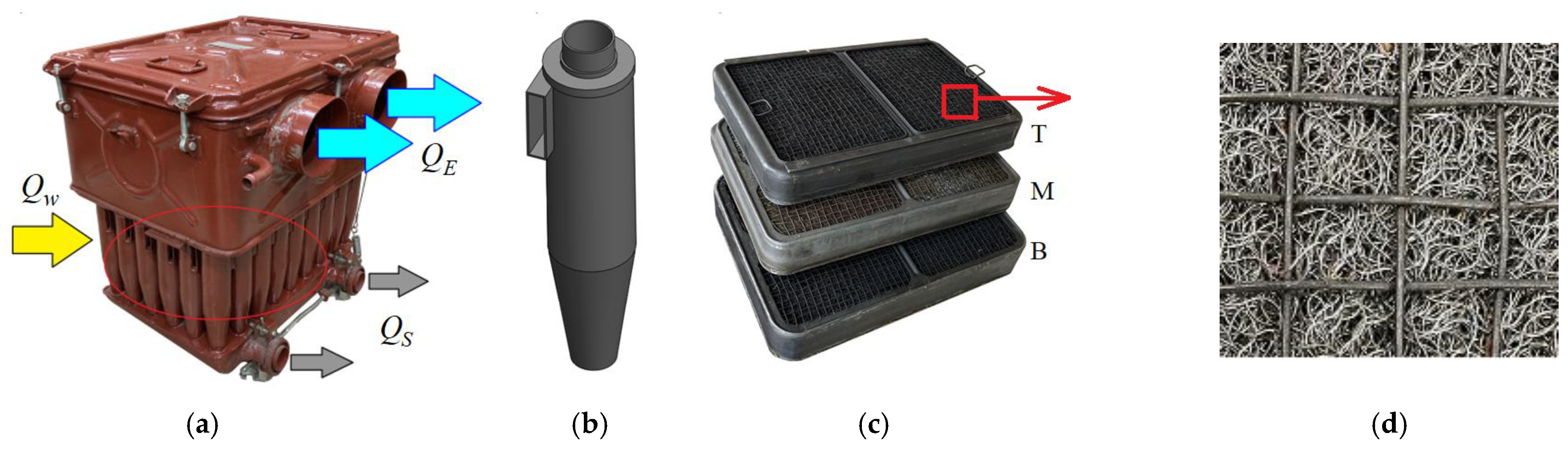
Two-stage air filters (Figure 4) working in the “multi-cyclone-porous partition” system and ensuring clean air intake to the engine, which is the power unit of the military caterpillar vehicles, constituted the subject of the research.

A multicyclone is made of several dozen return cyclones with a tangential inlet, while the second stage of filtration is a moistened filter bed in the form of three (bottom—B, middle—M, top—T) cassettes arranged in a series filled with an irregular, compressed bed of steel wire with a diameter of d_s = 0.25 mm. Filter bed thickness of the individual cassettes had the following values: 70 mm, 55 mm, 55 mm, respectively. Filtration speed in the cassettes, with the maximum air stream flowing through the filter, Q_max = 1800 m³/h, had a value of υ_F = 6 m/s. Such a large value is due to the small filtering cassettes area from the limited space available for the air filter inside the closed drive compartment.

The dust separated by cyclones falls to the bottom of the common settling tank, from where it is removed by ejection to the engine exhaust pipe, and then outside. The remaining dust part is transferred to filter cassettes, which must be serviced on a periodical basis. The servicing primarily consists of washing the filter cassettes (pouring a washing agent under pressure through them), drying them, and then submerging them (in order to moisten the wire surface) with engine or diesel oil heated to 60–100 °C. The presented technology of servicing air filters “multicyclone—moistened mesh bed” is labour-intensive, dangerous, and expensive.

The servicing should only be performed when filter cartridges loading with dust generates a pressure drop that results in excessive engine power loss. Due to the variable vehicle operating conditions, and mainly the variable value of dust concentration depending on terrain type, weather conditions, or the nature of vehicle use, it is difficult to predict a vehicle mileage at which such a moment will occur. For this reason, the air supply systems for many vehicles engines are equipped with sensors signalling that the filter has reached the admissible pressure drop Δp_f = Δp_fdop. This is the signal to perform the servicing. A lack of such signalling forces the filters to be operated in the planned-preventive system, i.e., after the mileage specified by the manufacturer. Due to different vehicle operating conditions, air filters’ maintenance is subject to maintenance, the current resistance of which slightly exceeds the initial filter resistance Δp_f0 and is significantly lower than the admissible resistance Δp_fdop, and the pressure drop of which has increased several times in relation to the initial one and is comparable and in extreme cases even higher than the admissible one.

Air filter pressure drop measurements were carried out on an everyday basis upon vehicle operation end, ensuring a stable engine thermal condition and measurements repeatability. Filter pressure drop measurements Δp_f were determined at the maximum engine vehicle rotational velocity n_N = 2000 rpm with an accuracy of 50 rpm, by repeating the measurement three times. These measurements’ average was used to analyse the results. The engine velocity was determined based on the readings of the on-board speedometer of the vehicle.

Pressure drop measurements were made with the use of an instrument, the basic component of which is a vacuum gauge with a measuring range of 0–20 kPa and an indication accuracy of 0.1 kPa.

3.2. Air Filters Research Results Analysis

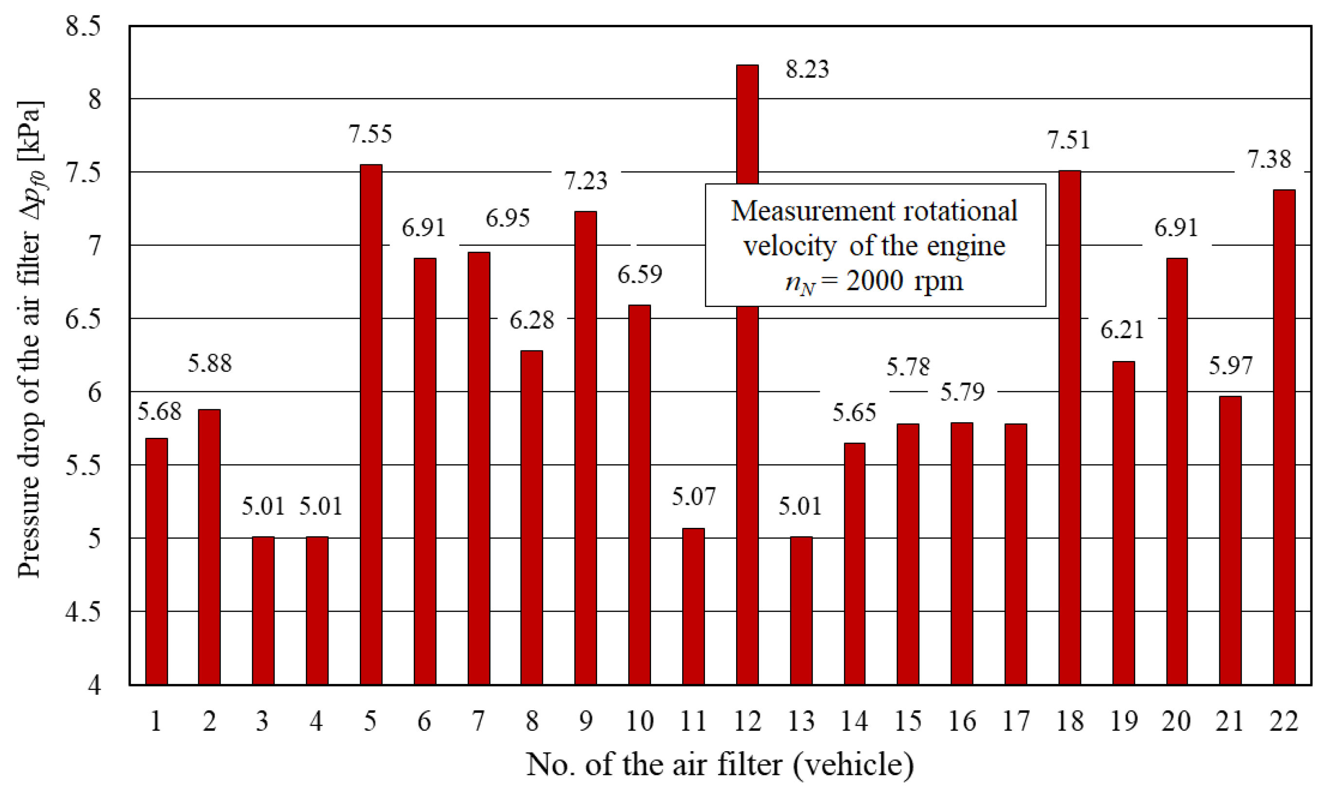
The research included 22 filters (in 22 caterpillar vehicles) that had been previously serviced. For such prepared air filters, their initial pressure drops Δp_f0 were determined. Considerable differences in the values of these initial pressure drops were found within 5–8 kPa (Figure 5).

The higher values of Δp_f0 (after servicing—washing the filter cassettes) significantly exceeding the initial pressure drop of the brand-new filters (which is within a narrow range of Δp_f0 = 4.1–4.2 kPa) were recorded for the filters operated in the vehicles for several years. This is due to the difficulty of completely washing away the dust from the densely packed and thick filter bed cassettes and the formation of hard-to-dissolve deposits on the bed wires of dust and oil, hardly removable by the washing technology applied (assumed as the instructions). With air filter operation time expiration, the mass of the unremoved sediments increases, and thus the initial pressure drop of the filter becomes higher and higher values frequently exceed twice the value of the pressure drop of the new filter; for example, in the case of filter No. 12—Δp_f0 = 8.23 kPa.

The high initial pressure drop virtually reduces the mileage reserve of the vehicle conditional upon the technical efficiency of the air filter, i.e., difference between the admissible pressure drop Δp_f0 and the initial pressure drop Δp_f0. For this type of filter and the mating engine of the caterpillar vehicle, the admissible pressure drop conditioned by a 5% decrease in engine power had value of Δp_f0 = 12 kPa [35].

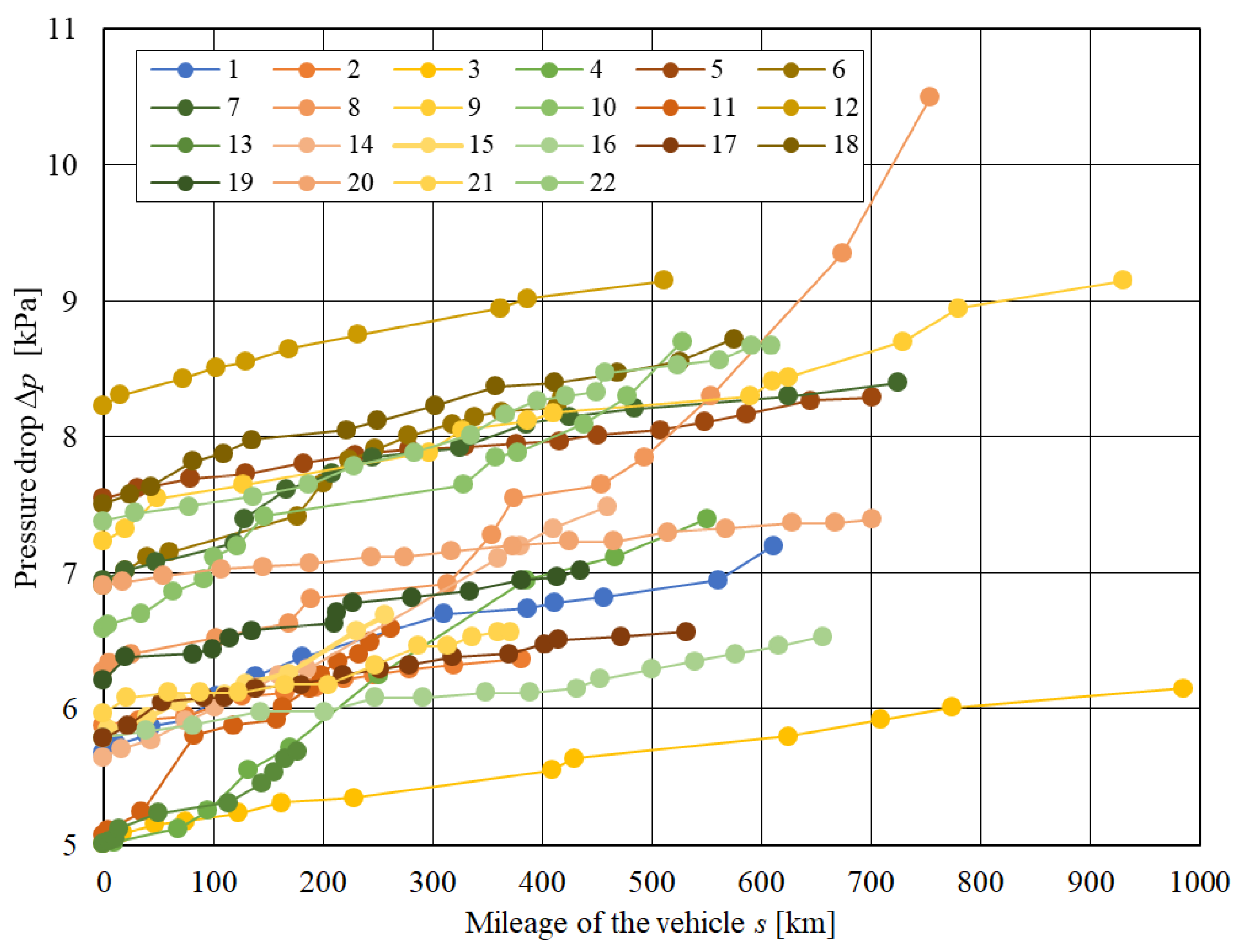
The number of kilometres travelled each day was different and resulted from the tasks performed. The vehicles in the observed research period achieved various mileages, not exceeding 1000 km. The research results are presented in Figure 6.

Among the analysed mileages, there are the ones whose shape for the entire curve line is visually the same—the nature of the increase in the value of the pressure drop is similar, whether in relation to the same values or to the changes in these values. Regrettably, for most of the mileages subject to the analysis, the value ranges with the clearly different natures are visible. Both ranges, with linear (with a different slope) and non-linear (sometimes concave, sometimes convex, with the inflection points) shapes of these mileages, can be distinguished. This may indicate radically different conditions of vehicle use between the measurements, i.e., driving with the different levels of air pollution: on grass, on sandy or rocky off-road, on dry or wet dirt road, platooning as the first vehicle (low air polluted) or as a subsequent vehicle (high dustiness in the air). The possibility of using the researched vehicles in such diametrically different conditions basically excludes drawing general conclusions about the intensity of pollution of the filtration barrier of the air filters, even for a single specimen. It is possible to assess this intensity and build a given model of the changes in pressure drop as a function of the vehicle mileage for the different filters used only under the same (possibly similar, but not significantly different) conditions. Each significant change in these conditions should result in the abandonment of the current model and the development of a new one. Information on the weather and road conditions between the measurements was unfortunately not recorded (which has resulted from research conditions), so visually noticeable changes in the value of the pressure drop of the filter cannot be related to the change in conditions of use of the vehicle. When modelling the course of these changes, a constancy of these conditions was arbitrarily assumed, and the models were built on the basis of all available experimental values, without dividing them into sets, giving visually the same nature of changes in the pressure drop.

It is easy to notice (Figure 6) that the mileages for which the measurements were made are very diverse, from less than 200 to almost 1000 km. The mileage values between measurements (from just a few to nearly 200 km) and measurements quantity for a single vehicle (from 9 for a total mileage of 257 km) to 17 (for a total mileage of 609 and 702 km) were also very irregular. This results in a highly differentiated density of performance, for example: for the 176 km mileage, 9 measurements were made, and for the approximately 5.5 times longer distance, 985 km—14 measurements, an increase by only 5.

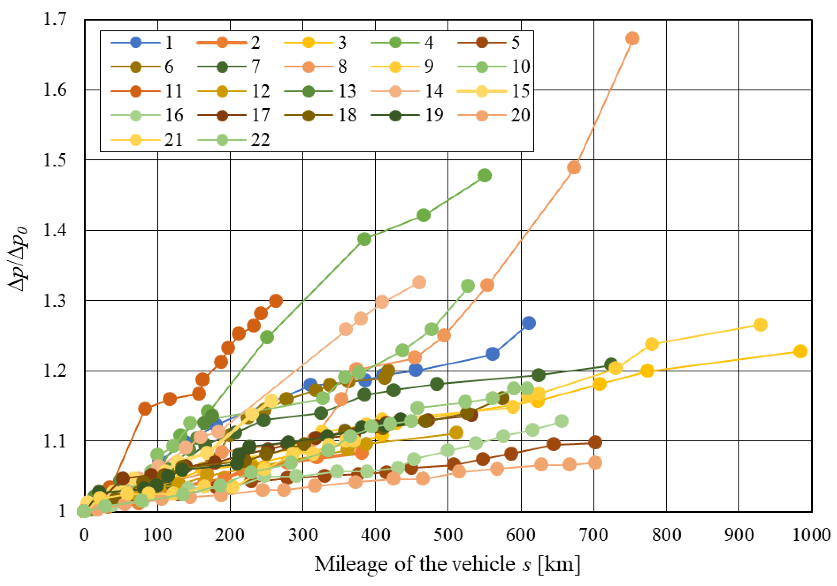
A difference in increase intensity in filter pressure drop value is also seen. The obtained mileages Δp = f(s) are not parallel (although it is noticeable for a large part of the mileages), but they intersect. These statements lead to the conclusion that these filters cannot be considered the same, which in turn makes it necessary to build individual models for each of them and excludes the possibility of building a generalised model for the filters of a concerned type. The conclusion about the impossibility of building a general model for the filter type is also confirmed by the curve line of the pressure drop value of the researched filters, shown in Figure 7 and Figure 8. In both of these figures, the mileages create the bunches of the curves arranged in a fan pattern. The observed changes in the value of the pressure drop of the researched filters are different, both in absolute and relative terms.

4. General Comments on the Usefulness of Modelling

Each technical product, including a machine, is manufactured for a specific purpose. This means that during the operation period, it should fulfil certain functions and meet the requirements defined by its designer or manufacturer. The scope and type of these requirements are specified in machine technical documentation in the form of basic operating parameters. In vehicles, these can be, for instance, engine power, maximum velocity, and fuel consumption. A set of values of such economic and machine technical parameters, determined during its construction and manufacturing for a given measure value of operation or within its specified range, determines machine technical condition. In the simplest case, two-state is assumed and states of fitness and unfitness for use are distinguished. They are unambiguously defined by the requirements contained in the technical documentation, and fitness is generally defined as the state in which the machine is capable of performing its functions according to the parameters specified in the technical documentation. The transitions between fitness and unfitness for use are called failures and repairs.

Technical diagnostics involves a problem of recognising the current, past, and future machine technical condition, while a diagnostic process itself is based on the results of the measurement values of the specific operating parameters, called the diagnostic parameters. It is worth recalling here that one of the properties required for a diagnostic parameter is its uniqueness. A threshold value of a diagnostic parameter dividing a range of the possible values of this parameter into ranges appropriate for the state of fitness and unfitness for use is called a limit value of this parameter. An output of the recorded values of the diagnostic parameter beyond the area appropriate for the condition of fitness, i.e., exceeding its limit value, corresponds to the machine entering the state of unfitness, i.e., its damage.

While repeating the measurements of the diagnostic parameter y of the machine for the successively larger values of the measure s of its operation (calendar time, working time, mileage, work cycles, fuel used, work done, etc.) and archiving their results, you have a certain set of data—the pairs of the values (si, yi), for which a regression model can be built with the a_j parameters:

y = f(s, a_j)

(3)

The forms of function f are usually elementary functions known from mathematical analysis (different functions are adequate to the experimental course to a different degree); due to the requirement of unambiguousness of the diagnostic parameter, monotonic functions are used here. The values of the a_j parameters are determined using data approximation methods, the most popular of which seems to be the method of least squares (the given form of the approximating function, i.e., the values of the a_j coefficients, is maximally adequate to the experimental course in terms of the approximation method used). The practical use of the obtained regression model is its inversion and determination of operation measure value, for which this model reaches any value within the range of its values; for example, the aforementioned limit value y_gr. The knowledge of operation measure value for which, according to the adopted regression model, the diagnostic parameter will reach its limit value

s_gr = f⁻¹(y_gr, a_j)

(4)

is extremely important for operation system management, when deciding on the allocation of a given machine to perform a specific work; if the s_gr is greater than machine value operation measure expected for assigned task completion (current sum value of the operation measure and operation measure value corresponding to the assigned task), it is highly probable that the machine will be subject to failure in the course of this task, resulting in the necessity to replace it with another machine and the necessity of its emergency transport to a repair service. Use of this probability concept is related to the adopted limit value of the diagnostic parameter, usually determined by some probabilistic method.

Assessment of modelling changes possibility in selected parameter value of the partition condition (metal, entangled wire) in vehicle air filter (i.e., the pressure drop of the filtered air reflecting a degree of its polluted with the captured, deposited matter) as a function of vehicle mileage (i.e., building the so-called regression models) was carried out based on data obtained for the 22 off-road vehicles designed for operation in various (difficult) operating conditions, including use in the areas with high dustiness. The vehicles were equipped with the same design filters. Due to the researched filters’ impossibility of self-cleaning, non-periodic increasing functions were selected for the modelling.

The method of least squares was applied to build the regression models, describing the obtained experimental mileage. In this sense, the obtained models are maximally adequate. The calculation algorithm contained in the MS Excel spreadsheet was used for a linear function, i.e., with two parameters—a slope factor and a shift factor. Therefore, it was assumed that all models will have functions with two parameters, while the data modelled with the non-linear functions required preliminary recalculation that enables functions’ use. When modelling the normalised mileages, whether absolutely or relatively, the initial value Δp₀ is a natural third parameter.

Due to the obtained experimental mileages (visually: linear, concave and convex), for the assumed limitation of the function parameters to two, the following functions were used as modelling functions.

1. Linear function:

y = as + b

(5)

The values y_i used for modelling purposes were: Δp_i, Δp_i − Δp₀ and Δp_i/Δp₀. Parameter values a and b were obtained with the use of MS Excel methods. The model values are determined from:

Δp_i = a₁s_i + b₁

(6a)

Δp_i = Δp₀ + a₂s_i + b₂

(6b)

Δp_i = Δp₀(a₃s_i + b₃)

(6c)

according to the modelled values.

2. Power function:

y = bs^a

(7)

For s = 0, function value y = 0. The values y_i used for modelling were Δp_i − Δp₀. It helped easily avoid the problem resulting from a required zero value of the model for s = 0. Then, the model described by the relationship

Δp = Δp₀ + bs^a

(8)

assumes the initial value Δp₀. This model use requires its linearization to the form:

ln(Δp − Δp₀) = ln(bs^a) = lnb + alns = B + aS = Y

(9)

where a—slope of the obtained straight line, B—shift factor of this straight line, Y and S—values obtained from:

Y = ln (Δp − Δp₀)

(10a)

S = lns

(10b)

It is a double logarithmic data representation. Model linearisation excludes the use of the starting point for modelling, because ln0 does not exist. A model shift factor after its linearisation B is related to the corresponding factor of the non-linear model b by an obvious relationship:

B = lnb.

(11)

Parameter values a and B are obtained according to MS Excel procedures. The value b is determined from:

b = e^B

(12)

The values of the model are determined from:

Δp_i = Δp₀ + bs_i^a

(13)

3. Exponential function 1a:

y = ba^s = be^slna = be^As = e^lnbe^As = e^Be^As = e^{B + As}

(14)

For s = 0, function value y = b. The values y_i used for modelling were Δp_i or Δp_i/Δp₀. Model use requires its linearisation to the form:

lny = ln(ba^s) = lnb + slna = B + As = Y

(15)

where A—slope of the obtained straight-line, B—shift factor of this straight line, Y—values obtained from the relationship:

Y = lny

(16)

This is a logarithmic data representation. Model linearisation excludes the use of the starting point for modelling, because ln0 does not exist. Model slope and shift factor after linearisation of A and B are related to the corresponding factors of the non-linear model a and b with obvious relationships:

A = lna

(17a)

B = lnb

(17b)

The values of the parameters A and B are obtained according to MS Excel procedures. The values a and b are determined from the relationships:

a = e^A

(18a)

b = e^B

(18b)

The values of the model are determined from the relationship:

Δp_i = b₁a₁^si

(19a)

Δp_i = Δp₀b₂a₂^si

(19b)

according to the modelled values.

4. Exponential function 1b:

y + 1 = ba^s = be^As = e^{B + As}

(20)

Values y_i used for modelling purposes had values of Δp_i − Δp₀. Since the initial data value is zero, it is required to add any positive number to all data (number 1 has been assumed in the research). Such data shift operation value has enabled to obtain a non-zero model value for s = 0. This model use requires its linearisation to the form:

ln(y + 1) = ln(ba^s) = lnb + slna = B + As = Y

(21)

where A—slope of the obtained straight-line B—shift factor of this straight line, Y—values obtained from:

Y = ln(y + 1)

(22)

It is a logarithmic shifted values representation. Model linearisation does not exclude starting point use for modelling. The slope and model shift factor after its linearisation A and B are related to the corresponding factors of the non-linear model a and b by the relationships (17). Parameter values A and B are obtained with the use of MS Excel procedures. Values a and b are appropriately determined from the relationship (18). Model values are determined from:

Δp_i = Δp₀ + ba^si − 1

(23)

5. Exponential function 2a:

y = e^{bs^a}

(24)

For s = 0, function value is y = 1. The values y_i used for the purposes of modelling were Δp_i/Δp₀, because only they equal 1 for s = 0. This model use requires its linearisation to the form:

ln(lny) = ln(bs^a) = lnb + alns = B + aS = Y

(25)

where: a—slope of the obtained straight line, B—shift factor of this straight line, Y and S—values obtained from the relationship:

Y = ln(lny)

(26)

S = lns

(27)

It is a double-logarithmic logarithm representation of relatively corrected value. Model linearisation excludes starting point use for modelling, because ln (ln1) = ln0 does not exist. The shift factor of the model after its linearisation B is related to the corresponding factor of the non-linear model b by the relationship (11). Parameter values a and B are obtained by MS Excel procedures. The value b is determined from the relationship (12). Model values are determined from:

Δp_i = Δp₀e^{bsi^a}

(28)

6. Exponential function 2b:

y + 1 = e^{bs^a}

(29)

The values y_i used for modelling purposes were Δp_i − Δp₀. Since the initial data value is zero, it is required to add a positive number to all data (number 1 has been assumed in the research). Such data shift operation value has enabled to obtain a non-zero model value for s = 0. This model use requires its linearisation to the form:

ln(ln(y + 1)) = ln(bs^a) = lnb + alns = B + aS = Y

(30)

where a—slope of the obtained straight line, B—shift factor of this straight line, Y and S—values obtained from the relationship:

Y = ln(ln(y + 1)

(31)

S = lns

(32)

It is a double-logarithmic logarithm value representation corrected relatively and shifted by 1. Model linearisation excludes starting point use for modelling, because ln(ln(0 + 1)) = ln0 does not exist. Model shift factor after its linearisation B is related to the corresponding factor of the non-linear model b by the relationship (11). Parameter values a and B were obtained by MS Excel procedures. The value b is determined from the relationship (12). Model values are determined:

Δp_i = Δp₀ + e^{bsi^a} − 1

(33)

7. Logarithmic function:

y = ln(bs)^a = aln(bs) = a(lnb + lns) = alnb + alns = B + aS

(34)

The values y_i used for the modelling purposes were Δp_i, Δp_i − Δp₀ or az Δp_i/Δp₀. This model use requires its linearisation to the form:

y = alnb + alns = B + aS

(35)

where A—slope of the obtained straight-line B—shift factor of this straight line, S—values obtained from the relationship:

S = lns

(36)

This is a logarithmic argument representation. Model linearisation excludes starting point use for modelling, because ln0 does not exist. The shift factor of the model after its linearisation B is related to the factors of the non-linear model a and b by an obvious relationship:

B = alnb

(37)

Parameter values a and B are obtained by MS Excel procedures. The value b is determined from the relationship (12). Model values are determined from:

b = e^B/a

(38)

Model values are determined from:

Δp_i = a₁ln(b₁s_i)

(39)

Δp_i = Δp₀ + a₂ln(b₂s_i)

(40)

Δp_i = Δp₀a₃ln(b₃s_i),

(41)

according to the modelled values.

It is obvious that increasing exponential models are concave, except for those with a power index (called exponential 2 in this paper) for 0 < a <1 (it is taken a root from the argument) and b > 0 and for a, b < 0. For these exceptions, the models used feature an inflection point. In these two exceptions, the smaller the a is, the more explicit the initial convexity and the less explicit the end concavity. The logarithmic models are convex. The power models are concave, linear or convex, depending on index value (convex for less than 1, linear for 1 and concave for greater than 1).

Changes of examples (for filter No. 14 according to Figure 5, Figure 6, Figure 7 and Figure 8) in the factors occurring in these models for an increasing number of the modelled data (according to an occurrence of the subsequent recorded filter pressure drop) are given in

Table 1. Obtained change models in pressure drop value Δp in selected vehicle air filters as mileage value function s.

Measurement Values Results			Model	(1)Δp= as + b		(3)Δp= bas		(4)Δp=Δp0 +bas− 1
no	s [km]	Δp [kPa]
1	0	5.65	Measurements	a	b	b	a	b	a
2	17	5.71	1–2	0.003529	5.650000	5.650000	1.000622	1.000000	1.003433
3	43	5.77	1–3	0.002751	5.654989	5.655063	1.000482	1.005364	1.002596
4	75	5.91	1–4	0.003377	5.646018	5.646761	1.000584	0.999581	1.003000
5	102	6.01	1–5	0.003531	5.642638	5.644064	1.000606	0.999171	1.003019
6	140	6.16	1–6	0.003657	5.638543	5.641409	1.000621	1.000777	1.002969
7	160	6.25	1–7	0.003756	5.634719	5.638799	1.000633	1.001519	1.002950
8	185	6.29	1–8	0.003640	5.640207	5.644821	1.000610	1.008728	1.002798
9	360	7.11	1–9	0.004034	5.610628	5.633081	1.000638	1.030405	1.002515
10	380	7.2	1–10	0.004117	5.60403	5.631010	1.000642	1.036220	1.002443
11	410	7.33	1–11	0.004158	5.600488	5.630812	1.000643	1.041105	1.002389
12	460	7.49	1–12	0.004138	5.602588	5.636023	1.000634	1.049925	1.002305
Model		(2)Δp=Δp0+ bsa		(5)Δp=Δp0ebs^a		(6)Δp=Δp0 +ebs^a− 1		(7)Δp= aln(bs)
Measurements		b	a	b	a	b	A	a	b
2–3		0.007229	0.746936	0.001293	0.741290	0.007645	0.716846	0.064656	1.33 × 1037
2–4		0.003708	0.963277	0.000674	0.952240	0.004256	0.906669	0.127580	1.42 × 1018
2–5		0.003170	1.011377	0.000582	0.997409	0.003801	0.941327	0.162429	9.01 × 1013
2–6		0.002904	1.036841	0.000540	1.019369	0.003666	0.951856	0.204944	5.61 × 1010
2–7		0.002746	1.052652	0.000515	1.032609	0.003599	0.957105	0.236503	1.29 × 109
2–8		0.002831	1.044324	0.000534	1.022847	0.003785	0.943250	0.254396	2.28 × 108
2–9		0.002609	1.064799	0.000514	1.032124	0.004045	0.926552	0.403062	43,424.3
2–10		0.002512	1.074232	0.000507	1.035859	0.004195	0.917470	0.479454	4185.44
2–11		0.002460	1.079460	0.000504	1.037061	0.004322	0.910104	0.534354	1172.35
2–12		0.002461	1.079358	0.000511	1.033640	0.004501	0.900222	0.580821	479.0153

.

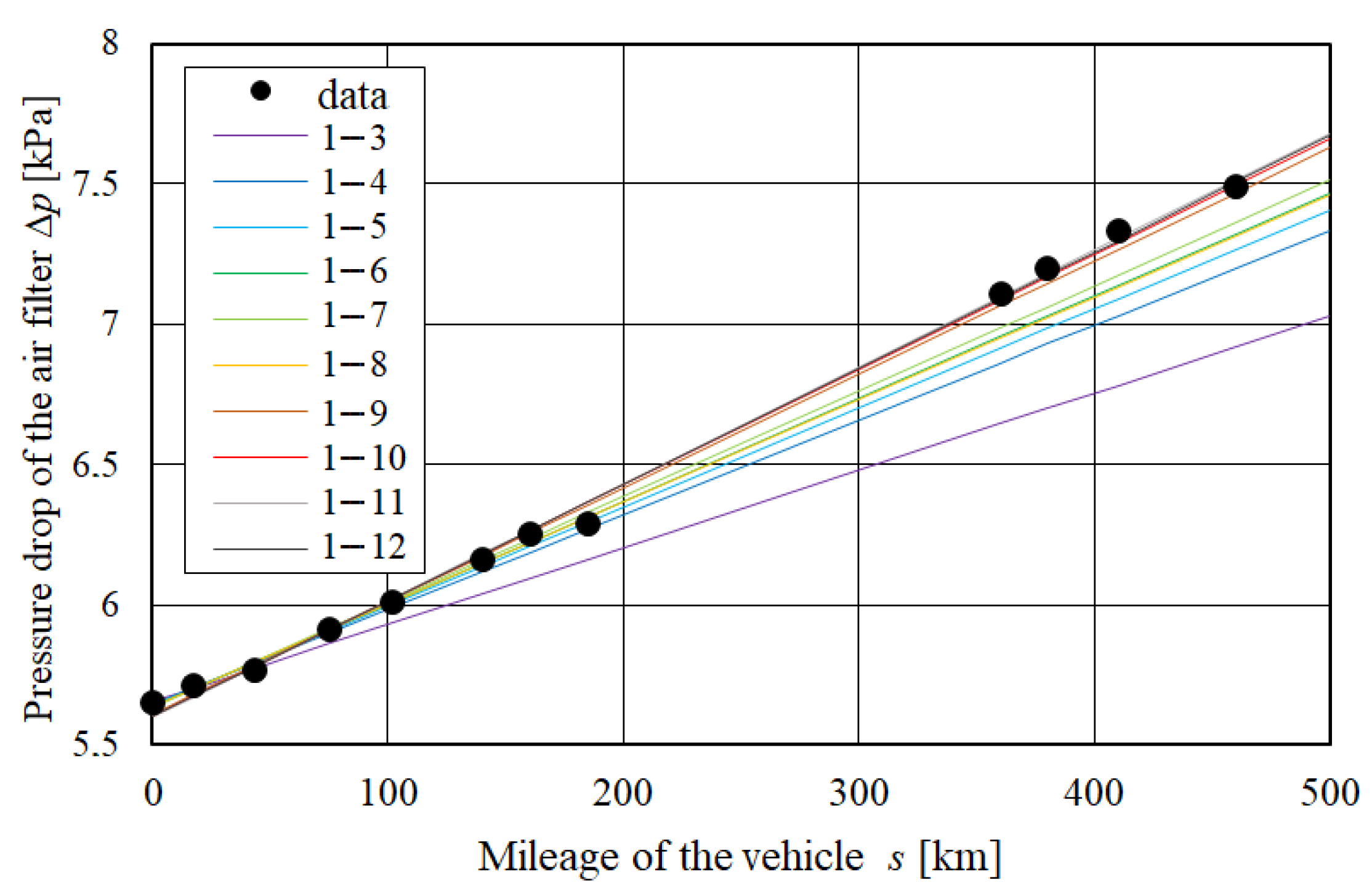
In Figure 9 and Figure 10, changes in selected models shape (i.e., exponential 2a: y = e^{bs^a} and linear y = as + b) an increasing measurement results number used for modelling. It is clearly visible that as a range of the modelled experimental data increases (obtaining the newer and newer measurement results), model forms are corrected. This correction value is not large (changes in the first significant digit only by 1, sometimes changes only in the fourth significant digit). The exception here are logarithmic models for which changes by several orders of the value were obtained. However, logarithmic function nature is too non-linear to be used to model changes in air filters pressure drop, which will be pointed out. Model forms obtained for the full analysed mileage in case of this example are as follows:

• Δp = 0.004138s + 5.602588 ≈ 0.0041s + 5.60,
• Δp = 5.65 + 0.002461s^1.079358 ≈ 5.65 + 0.0025s^1.08,
• Δp = 5.636023 × 1.000634^s ≈ 5.64 × 1.000634^s,
• Δp = 5.65 + 1.049925 × 1.002305^s − 1 ≈ 4.65 + 1.05 × 1.0023^s,
• Δp = 5.65e^{0.000511s^1.033640} ≈ 5.65e^{0.000511s^1.03},
• Δp = 5.65 + e^{0.004501s^0.900222} − 1 ≈ 4.65 + e^{0.0045s^0.9},
• Δp = 0.580821ln (479.015s) ≈ 0.58ln(479s).

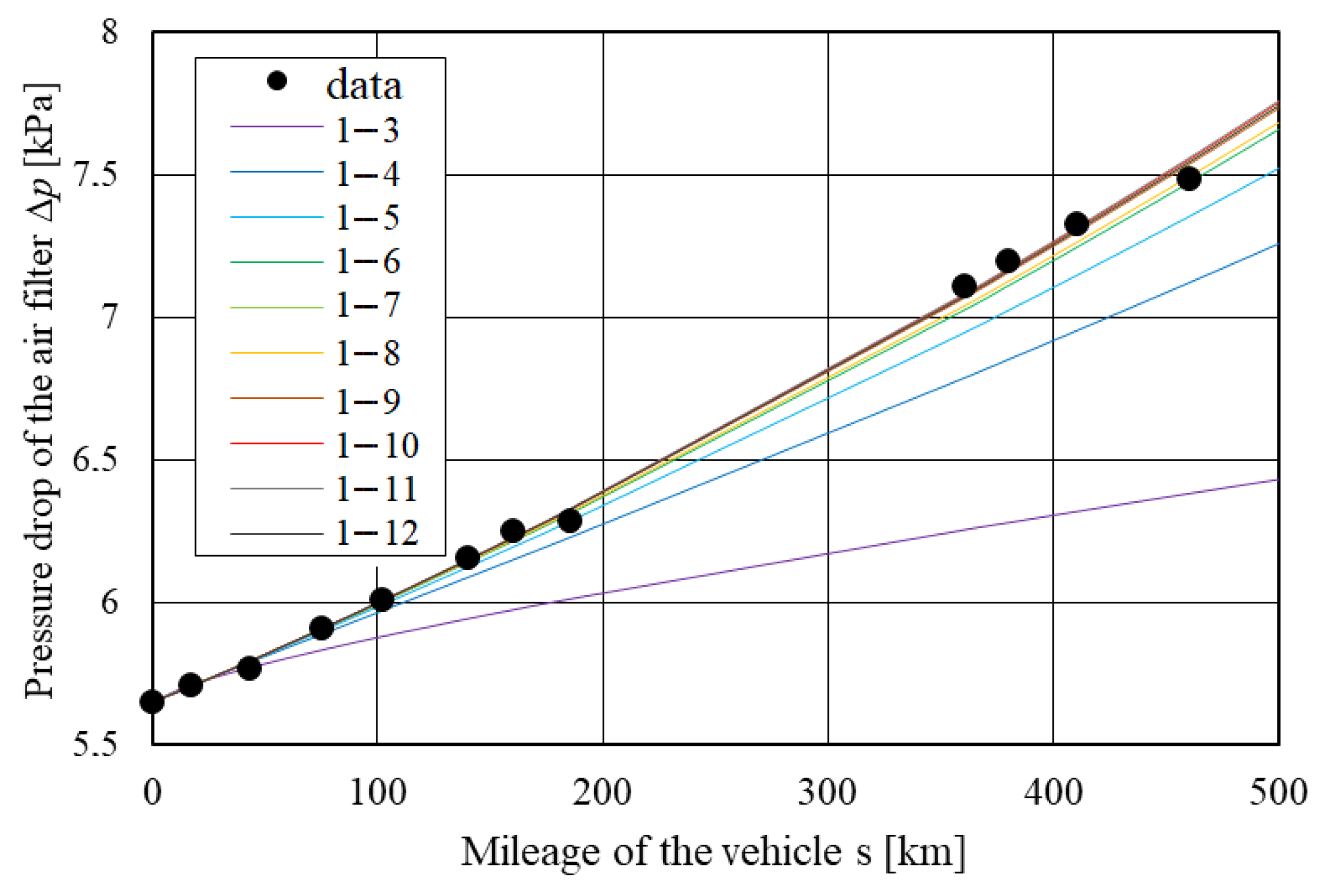
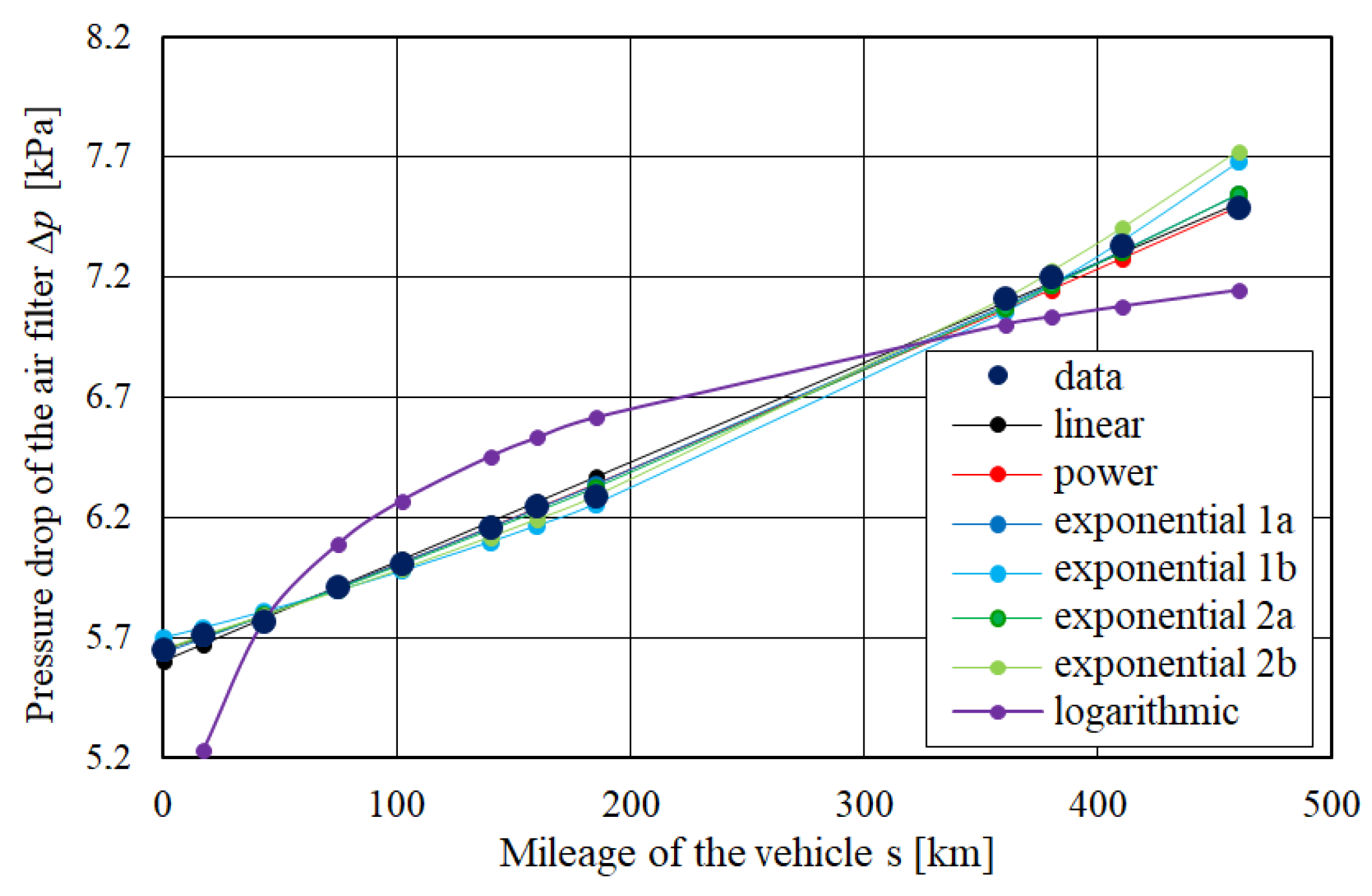
Model graphs against measurement result values are presented in Figure 11. On visual assessment basis of the presented curves, it can be concluded that in spite of the differences in the form of the functions describing them, all, except for the logarithmic model, model the experimental mileage quite well.

In numerical terms, a matching degree of the considered models to the experimental data was stated by value determination of the correlation coefficient between the experimental values and the values obtained on the basis of the designated models.

Table 2. Correlation values coefficient between the experimental and modeled pressure drop values Δp of selected air filters with a visually constant shape (for increasingly lower correlation coefficient values, bold black, black, blue, green, purple, brown and red colors were used).

Experimental Values in The Coordinate System s [km] − Δp [kPa]	Data Range	Model Correlation Coefficient Values (×0.001)
		1	2	3	4	5	6	7
	to 5	992	998	991	988	998	998	972
	to 6	995	995	995	992	996	997	944
	to 7	994	997	993	986	997	998	933
	to 8	991	998	989	977	999	999	918
	to 9	994	998	993	984	999	999	918
	to 10	991	999	989	977	999	998	923
	to 5	996	996	996	998	996	997	942
	to 6	997	998	998	999	998	999	935
	to 7	998	999	998	999	999	999	935
	to 8	997	997	997	995	997	996	943
	to 9	997	998	999	996	999	998	864
	to 10	998	999	999	997	999	999	881
	to 11	998	955	999	997	1000	999	894
	to 12	999	999	999	995	999	997	904
	information contained in Table 1 and Table 4, and shown in in Figure 6, Figure 7 and Figure 8 relates to this vehicle

presents this coefficient values for the examples of experimental mileages characterised by a visually similar (constant) shape for the entire mileage curve, sequentially for an increasing modelled data number, starting from the datasets ending with measurement 5—out of the 22 analysed experimental mileages, only 7 were identified (Table 2 shows values for two of them).

Table 3. Coefficient values between the experimental and modeled pressure drop values Δp of selected air filters with a visually variable shape (for increasingly smaller correlation coefficient values, bold black, black, blue, green, purple, brown and red were used).

Experimental Values in the Coordinate System s [km] − Δp [kPa]	Data Range	Model Correlation Coefficient Values (×0.001)
		1	2	3	4	5	6	7
	to 5	975	984	974	970	983	983	949
	to 6	983	979	984	986	979	981	892
	to 7	991	988	992	994	988	990	893
	to 8	995	994	995	994	994	995	905
	to 9	991	994	988	973	992	987	914
	to 10	981	987	976	958	985	976	933
	to 11	981	948	976	961	985	978	944
	to 12	979	987	974	959	985	977	952
	to 13	974	985	968	948	982	972	957
	to 14	980	969	975	958	986	979	951
	to 5	792	993	790	783	993	993	920
	to 6	863	976	862	857	976	976	860
	to 7	973	979	871	866	979	980	896
	to 8	915	900	916	917	900	901	761
	to 9	927	877	929	936	877	879	747
	to 10	947	904	949	955	904	907	782
	to 11	958	910	959	966	920	923	800
	to 12	965	932	967	974	933	937	816
	to 13	971	943	973	978	944	947	830

presents coefficient values for two selected mileages with different (visually variable) mileage curves (with the intervals of the linear (with the different gradients) and non-linear (sometimes concave, sometimes convex, with the inflection points) mileage curves shapes.

The data contained in these tables confirms good modelling visual assessment of the experimental mileages and its similar quality—correlation coefficient obtained values are high (except for those specified for logarithmic models, they are not less than 0.9 and in a significant number of the cases they are close to one), the differences between them occur at the 2nd and 3rd, and even at the 4th and 5th fractional decimal places. For experimental mileages with visually constant shapes, model orders from the point of view of the degree of their matching to the experimental mileages is rather constant as modelled data scope increases, and for mileages with the variable shapes, the order changes depending on the changes in experimental mileage curves shapes.

5. Regression Models Use to Forecast Changes in Filter Pressure Drop and Technical Condition

As stated in the introduction, a practical sense of building regression models is diagnostic parameter values’ predicting possibility, and thus inferring about the future technical machine condition, and in case of having diagnostic parameter limit value, also about operation margin until the machine reaches failure state. For the purposes of assessing, predicting quality can be used the simplest, apparently obvious measure, which is the difference between the predicted value Δp_i by a given model for the value of the operation measure s_i, for which the next research has been performed, and the recorded value Δp_ie in this research, which can be called the absolute prediction error B_i:

B_i = Δp_i − Δp_ie.

(42)

The relative prediction error b_i can also be determined:

b_i = (Δp_i − Δp_ie)/Δp_ie.

(43)

With such elements defined order in these differences, the obtained error sign value is significant. If this value is positive, it means that the concerned model overstates the predicted value in relation to the real one, and therefore it is too close to the fact that the failure occurs. If the value is negative, it is otherwise. Since the error values are determined on an ongoing basis, according to the occurrence of the successive measurement results (for a set of n measurements, the model form is determined, after performing another, n + 1, measurement for the operation measure s_{n + 1}, this model value is determined, which is compared with the value measured, and a new model form is determined, from which the value for the operation measure s_{n + 2} is determined, etc.), then for the obtained set of error values, their average level can be determined as their modules’ arithmetic mean (where the determined errors feature the different signs, this average will not be zero).

Table 4. Pressure drop values Δp of the selected air filter with a visually constant shape registered and predicted on the basis of two selected models.

Measurement Results Δpie [kPa]	Linear Model: Δp = as + b			Exponential Model 2a: Δp = Δp0ebs^a
	Prediction Δpi [kPa]	Error Bi [kPa]	Error bi [%]	Prediction Δpi [kPa]	Error Bi [kPa]	Error bi [%]
5.77	5.802	0.032	0.551	-	-	-
5.91	5.861	−0.049	−0.824	5.832	−0.078	−1.316
6.01	5.99	−0.020	−0.325	5.97	−0.040	−0.659
6.16	6.137	−0.023	−0.374	6.123	−0.037	−0.594
6.25	6.224	−0.026	−0.421	6.215	−0.035	−0.563
6.29	6.33	0.04	0.629	6.326	0.036	0.568
7.11	6.951	−0.159	−2.240	7.039	−0.071	−1.000
7.2	7.143	−0.057	−0.786	7.158	−0.042	−0.585
7.33	7.292	−0.038	−0.516	7.311	−0.019	−0.253
7.49	7.513	0.023	0.312	7.559	0.069	0.927
average error level		0.0466	0.698		0.0474	0.718

shows absolute and relative error values (multiplied by 100%) for predicting the value of the selected air filter with a visually constant shape (see Table 1 and Figure 9, Figure 10 and Figure 11) based on two selected models: linear and exponential 2a, updated on an ongoing basis, with first values row corresponding to the models determined on the basis of only two recorded values and the prediction with regard to the third value.

As can be noticed, for the presented example, the prediction is quite good—the prediction error does not exceed 1% of the real value, except for predicting with a large prognosis horizon (nearly nine times longer than others). While comparing the obtained prediction error values to correlation coefficient value between the experimental and modelled values for this filter (the fourth in Table 2—Filter No. 14), it can be perceived that the better model correlation with the experimental data will not necessarily result in better predicting—a correlation concerns known data, and predictive data refers to the data not known yet, with the values depending on the unpredictable changes in the machine operating conditions. In the example presented, correlation coefficient values are greater for the exponential model 2a than for the linear one, but prediction average relative error based on the linear model is less than this level for the exponential model 2a.

6. Conclusions

Non-decreasing change course in air pressure drop value in vehicle filters, as a vehicle mileage function, imposes increasing monotonic functions’ selection for development of regression models in respect to these changes. Linear functions, power, exponential and logarithmic with two parameters were applied in the research, which enabled to use the least squares method, implemented in a popular and broadly available spreadsheet, in order to determine these parameters’ value.

All monotonic functions with parameters obtained by the use of least squares method as pressure drop regression models for vehicle filters resulted in large correlation coefficient values between the modelled (experimental) and model (calculated) values. The lowest correlation for the modelled experimental data was usually obtained for the logarithmic models.

Pressure drop diversification value of the researched filters forces the development of each model on an individual basis. It is obvious that these models must be modified for constantly obtained new modelled data values. Observed variability in the shape of experimental air pressure drop curve lines of some researched filters probably results from vehicles usage in considerably changing road conditions (i.e., in significantly different level conditions of polluted filtered air, with vehicle usage periods in clean air and vehicle usage periods in very dusty air). Conditional mood usage here results from a lack of unequivocal information about road conditions by vehicles between filter pressure drop measuring moments. Obtaining such information would require continuous road monitoring conditions (e.g., air dust in air intake vicinity), which was impossible during the experiment. In subsequent papers, developing regression models possibility on the basis of a certain number (necessary to determine) of the last measurements should be considered. Certainly, this approach is also not entirely satisfactory and will not provide models that perfectly reflect road conditions variability.

The correlation degree of linear and non-linear models with experimental data is similar. Similarly, error rates related to predicting the actual air filter pressure drop values are similar. Therefore, it seems reasonable to state that a linear function can be used to model this pressure drop (pressure drop change, as vehicle mileage function is linear). This conclusion simplifies modelling and predicting operations as it eliminates the need to linearise non-linear models (the number of mathematical operations necessary to define the model is lower). Resignation from the use of non-linear models is also substantiated by vehicle use in considerably changing road conditions. This, in turn, causes increased rate differences in air pressure drop value at the filter, related to its clogging by the filtered pollutants—for vehicle use in air that is gradually cleaner, pressure drop convex shape changes are obtained, and in air that is gradually more polluted, pressure drop concave shape changes are obtained. Therefore, for cyclical change in the degree of air purity over a longer usage period, linear model adoption as a certain averaging of the cyclically adequate concave and convex models seems to be substantiated.

According to the authors, dynamically variables’ determination, individual regression models in respect of individual vehicles—linear or non-linear ones—is of great importance, as it gives the opportunity to move from a planned and preventive strategy for air filters’ use in special vehicles used in variable dustiness conditions (often high, for example, in deserts) to strategies according to their actual technical condition. This will make the vehicle maintenance system more flexible. The presented mathematical apparatus itself is so simple that it can be used by any engineer supervising the vehicle operation process, employing commonly available computing environments, for example, spreadsheets that are part of office suites. It is also possible to develop simple applications intended for the mobile devices that carry out appropriate calculations in order to obtain information about the estimated vehicle mileage up to the value in which it is necessary to perform servicing (for example, cleaning) of a concerned air filter.