Abstract
Investigation of the change rate for contaminant parameters is important to characterize dense non-aqueous phase liquid (DNAPL) transport and distribution in groundwater systems. In this study, four experiments of perchloroethylene (PCE) migration are conducted in two-dimensional (2D) sandboxes to characterize change rates of PCE saturation (So) and PCE–water interfacial area (AOW) under different conditions of salinity, surface active agent, and heterogeneity. Associated representative elementary volume (REV) of the change rate of So (So rate) and change rate of AOW (AOW rate) is derived over the long-term transport process through light transmission techniques. REV of So rate (SR-REV) and REV of AOW rate (AR-REV) are estimated based on the relative gradient error (). Regression analysis is applied to investigate the regularity, and a model based on a back-propagation (BP) neural network is built to simulate and predict the frequencies of SR-REV and AR-REV. Experimental results indicated the salinity, surface active agent, and heterogeneity are important factors that affect the So rate, AOW rate, SR-REV, and AR-REV of the PCE plume in porous media. The first moment of the PCE plume along the vertical direction is decreased under conditions of high salinity, surface active agent, and heterogeneity, while these factors have different effects on the second moment of the PCE plume. Compared with the salinity and surface active agent, heterogeneity has the greatest effect on the GTP, the distributions of the So rate and AOW rate along the depth, and dM, dI. For SR-REV, the standard deviation is increased by the salinity, surface active agent, and heterogeneity. Simultaneously, the salinity and heterogeneity lead to lower values of the mean value of SR-REV, while the surface active agent increases the mean value of SR-REV. However, the mean and standard deviation of AR-REV have no apparent difference under different experimental conditions. These findings reveal the complexity of PCE transport and scale effect in the groundwater system, which have important significance in improving our understanding of DNAPL transport regularity and promoting associated prediction.
1. Introduction
With the development of the social economy and urbanization, extensive use of dense non-aqueous phase liquids (DNAPLs) in the industry has led to serious groundwater environment deterioration, which has become one of the hotspots that attracted attracting global attention [1,2,3,4,5,6,7,8]. When these toxic, carcinogenic, and less easily degraded DNAPLs cause groundwater contamination, the ecosystem and human health are seriously threatened [9,10,11,12]. DNAPLs are heavier than water and usually migrate downward through the saturated zone due to their greater density. DNAPLs can be trapped as residual ganglia and globules and accumulate pools at permeability barriers in groundwater systems [13,14,15]. In this infiltration process, DNAPLs form the a heterogeneous distribution. As a result, residual and pooled DNAPL become persistent contaminant sources, which can cause long-term groundwater contamination and high risk for to ecosystems and human health. Landrigan et al. [5] reported that nine million people died in 2015 caused bydue to the influence of environmental contamination. Contamination caused by DNAPLs can lead to various diseases such as heart disease, stroke, cancerr etc. [5,16]. Indeed, effective remediation relies on understanding the characteristics of DNAPLs migration and distribution in the aquifer [8,12,17]. Therefore, investigation of the change rate of DNAPLs concentration and its associated characteristics is fundamental to enhancing understanding of the regularity of DNAPL transport and remediation [17].
Modeling contaminant transport in porous media is based on the continuum assumption, by with the help of representative elementary volume (REV) [18,19]. REV is indispensable for modeling contaminant transport in groundwater and deriving associated effective macroscopic parameters. High High-quality experiments can improve our understanding of the characteristics of the REV for porous media and inner contaminants [20,21]. With the development of techniques, light transmission techniques (Figure 1a) gained popularity for the measurement of parameters of translucent porous media, contaminants migration behavior, and REV estimation [20,21,22,23,24]. Light transmission techniques can overcome the limitations associated with X-ray measurement and gamma-ray radiation, such as high costs, hazardous working environments, and the special requirement of high energy sources, which facilitates REV estimation for the DNAPL plume [21]. Figure 2b presents a conceptual representation of the REV curve to reveal the change of media parameters as the measured scale increased. When the measured scale (L) (Figure 2c) is close to the REV region (Lmin ≤ L ≤ Lmax), the value of the parameter is relatively constant and steady. Upon further decrease (L < Lmin) and increase (L > Lmax) of the spatial scale, the value of the parameter will become nonstationary and unsteady. However, the REV plateau in region II is difficult to identify for a real porous media system, which causing the associated study studies to be only limited to only a few natural porous media and for a single variable due to various difficulties and complexity [18,19]. The REVs of the change rate of DNAPL concentration and its associated characteristics during long-term transport periods under different conditions have not been explored. As a result, it is very essential to study the REVs of the change rate of DNAPL saturation and the DNAPL–water interfacial area over a long time in the groundwater system for the improvement of in understanding DNAPL behaviors and designing more effective remediation schemes.
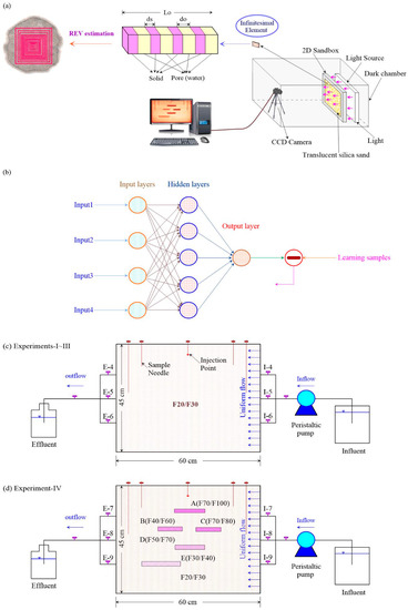
Figure 1.
(a) Schematic diagram of light transmission technique; (b) BP neural network structure containing four input layers, five hidden layers, and one output layer; (c) the two-dimensional (2D) sandbox system used by Experiments I~III; and (d) 2D sandbox system used by Experiment IV.
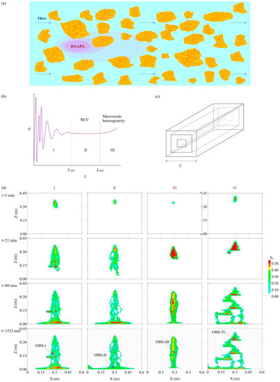
Figure 2.
(a) Conceptual schematic of DNAPL transport process in porous media; (b) cConceptual representation of the measured value of the variable under different scales [19]; (c) tThe image window geometry of core-centered cuboid used by REV estimation; and (d) PCE saturation of Experiments I~IV derived from light transmission technique during the entire experimental period and observation cells.
A bBack-propagation (BP) neural network is a nonlinear learning system equipped with self-learning capacity [25,26]. The basic principle is to use the error after the output to estimate the error of the direct leader layer of the output layer, and then use this error to estimate the error of the previous layer [24,27,28]. The application of the artificial neural network theory has made remarkable progress, especially in the fields of artificial intelligence, automatic control, computer science, information processing, robotics, and pattern recognition [27,29,30]. In recent years, the BP neural network is has been applied in the field of engineering, and achieved a series of research results. Ercanoglu [29] used a BP artificial neural network to assess the sensitivity of the SE Bartin (Turkey) landslide in the West Black Sea region. Polykretis et al. [30] found the average accuracy of prediction of landslides based on artificial neural networks for the Creole River Basin reached 84%. With the development of the artificial neural technique, the BP neural network has been widely used in the evaluation and prediction for of multiphase flow in porous media [27], data fusion for satellites [25], inverse modeling of groundwater flow [24], simulation of soil water dynamics [28], and dispersivity analysis [26]. However, few studies have addressed the simulation and prediction of the REV of the DNAPL plume by the neural network.
The objective of this research is to estimate and simulate the REVs of the change rate of DNAPL concentration and its associated characteristics under different conditions of salinity, surface active agent, and heterogeneity in the groundwater system. Four PCE transport experiments are performed in two-dimensional (2D) sandboxes packed by translucent porous media. The change rates of PCE concentration (So), PCE–water interfacial area (AOW), and associated REV sizes are quantified by light transmission techniques [20,21,22,23] and relative gradient error (ε_g^i). Afterward, a BP neural network is established to predict mean values of REV for PCE plume under different experimental conditions.
2. Materials and Methods
2.1. Experiment Procedure
Four experiments are performed in two-dimensional sandboxes to study the So-rate rate, AOW-rate rate, and associated REV under different conditions (Figure 1c,d). The sandboxes used by in Experiments -I~III are packed by with single F20/30 mesh translucent silica sand to create a homogeneous condition (Figure 1c), and the sandbox used by in Experiment-Experiment IV is packed with six kinds of translucent silica sand to create a heterogeneous condition (Figure 1d). F20/30 mesh translucent silica sand is used as background porous media for Experiment-IV. Moreover, five lenses with low permeability are added into the sandbox to create heterogeneity. For all experiments, water is pumped into sandboxes through influent ports (I1-3 and I4-6) and flows out through the effluent ports (E1-3 and E4-6) with the help of a peristaltic pump. The water flow velocity in sandboxes is kept at a constant rate of 0.5 m/d along the horizontal direction, which is similar to the natural groundwater flow rate. When the sandbox is fully saturated by with water, a light source is placed on the side of the sandbox to let light transit through translucent 2D porous media. A thermoelectrically air-cooled charge-coupled device (CCD) camera is placed on the other side of the sandbox to capture the emergent light intensity. Afterward, PCE is injected into the sandbox by a syringe pump to let PCE infiltrate and transport in the 2D sandbox (Figure 2a). The parameters of translucent porous media, inner PCE saturation (So), and So-rate rate of PCE plume are quantified using light transmission techniques [20,21,22,23]. Experiment-I is conducted under the condition of homogeneous porous media and low salinity. Experimental conditions of Experiments-II~IV are changed to study the effect of salinity, surface active agent, and heterogeneity. The detailed experimental conditions are given in Table S1.
2.2. REV Evaluation
Porosity of translucent porous media and PCE saturation (So) of PCE plume are quantified by light transmission techniques [20,21,22,23]:
where θ is porosity; Is is the emergent light intensity when light transmits through 2D translucent silica sand fully saturated with water; β and γ are two constant parameters [21]; I is the light intensity after light penetration through 2D porous media system including water, PCE, and solid; Ioil is the light intensity after light penetration through 2D translucent silica sand fully saturated with PCE; and So is PCE saturation. The assumption that the translucent silica sand surfaces are fully wetted by water allows the surface area of the PCE phase to be taken as the total PCE–water interface. PCE–water interfacial area (AOW) is normalized by the associated system volume (cm−1).
Based on the quantification of light transmission techniques, So-rate rate and AOW-rate rate are obtained as follows:
where and are PCE saturation at times and , respectively; and are PCE–water interfacial area at times and , respectively. Details about the spatial moment, GTP analysis, and REV estimation method are provided in Supplementary Materials.
2.3. BP Neural Network
Artificial neural network is a research direction in the field of artificial intelligence, which simulates the response of the brain through several neurons [24]. The BP neural network structure is a multi-layer feed-forward model in which many neural units are linked to each other to form a simulated biological neural network [26,27,28,29,30]. The neural network is a nonlinear learning system equipped with self-learning capacity [25,26,28]. It uses the mathematical modeling method, when the external information is obtained, the information is simply processed, and the processed result is input to the next layer of neurons until the output result.
The structure between layers is divided into three layers: an input layer that accepts external information, an intermediate hidden layer for information transmission and processing, and an output layer that outputs the final result [24,25,26,27,28]. Each layer is generally composed of one or more neurons, and each layer of neurons only receives the information transmitted by the neurons of the previous layer. The input layer accepts input information from the outside world. The nodes of the hidden layer only accept the input of information from the input layer. This structure determines that the BP neural network is sensitive to the neurons in the upper and lower layers, and among them, it has a greater impact on the information transmitted by the superior neurons [24,26,28]. To predict the REV of the PCE plume, a BP neural network is built, which includes four input layers, five hidden layers, and one output layer (Figure 1b).
3. Results and Discussion
3.1. So Rate and AOW Rate of PCE Plume
When PCE is injected into 2D translucent silica sand, PCE infiltrates vertically from the upper layer to the lower layer like a drop of water at in the first few minutes (Figure 2d). Afterward, PCE continues to infiltrate along a vertical direction for Experiments-I~III under homogeneous conditions. However, PCE pools on top of the five lenses in the heterogeneous porous media for Experiment -IV (Figure 2d). As PCE migration progresses, PCE cascades over the sides of lenses and reaches the bottom. The So-rate rate and AOW-rate rate of the PCE plume during the entire experimental period are derived based on light transmission techniques (Figure 3a,b). Through the distribution of the So-rate rate and AOW-rate rate, the place where migration is active can be identified. Before t = 80 min, the So-rate rate and AOW-rate rate of the PCE plume are relatively high. After t = 80 min, the So-rate rate and AOW-rate rate are kept at a low level, while PCE plumes have slight movement at in some places, such as the lower part of the PCE plume (Figure 3b). Then Then, migration becomes slower, and the PCE plumes are kept in a steady state for a long time until t = 1523 min (Figure 3b).
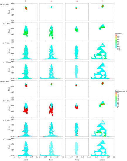
Figure 3.
(a) The change rate of PCE saturation for four experiments; (b) the change rate of PCE–water interfacial area during the entire experimental period.
The moment analysis, the results of the contaminated plume area, the GTP, and the associated regression analysis are presented in Figure 4a–f. In Figure 4a, there is a positive correlation between infiltration depth and injected PCE volume. The Salinity salinity has no obvious influence on the relationship between infiltration depth and injected PCE volume, while the surface active agent and heterogeneity have an apparent influence. When the injected PCE volume is the same, the infiltration depth of the PCE plume in Experiment-Experiment III (surface active agent) becomes lower, and Experiment-Experiment IV (heterogeneity) further reduces the infiltration depth of the PCE plume. Similarly, the surface active agent and heterogeneity also lower the σz of the PCE plume (Figure 4b). In Figure 4c, compared with Experiment-Experiment I, σxx of PCE plume is increased by heterogeneity (Experiment-Experiment IV) and is decreased when the surface active agent exists (Experiment-Experiment III). Moreover, σzz of the PCE plume has a larger value in Experiment-Experiment II when the salinity is high (Figure 4d), while surface active agent and heterogeneity all decrease the value of σzz. For the plume area, there is no obvious difference among Experiments-I, II, and IV, while the plume area is slightly small for Experiment-Experiment III under the condition of high concentration of surface active agent (Figure 4e). BesidesIn addition, the most important factor that affects the GTP of the PCE plume is heterogeneity (Figure 4f).
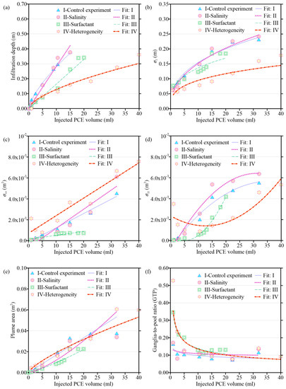
Figure 4.
Moment analysis of PCE plume and fitted models: (a) infiltration depth; (b) vertical first-order moment; (c) horizontal second-order moment; (d) vertical second-order moment; (e) plume area; and (f) GTP.
The change of the So-rate rate and AOW-rate rate along the depth for location x = 0.30 m is shown in Figure 5a. The peak value of the So-rate rate moves from top to bottom as time goes on. However, the change of the So-rate rate with the depth is very different for Experiment-IV (heterogeneity). The peak of the So-rate rate is very apparent at t = 21 min and t = 80 min for Experiment -IV. In addition, the AOW-rate rate has no apparent change as the depth increases for Experiment-IV, while the AOW-rate rate curves have some peaks for Experiments-I~III. These phenomena indicate that heterogeneity has the biggest influence on the distribution of the So-rate rate and AOW-rate rate along the depth for location x = 0.30 m.
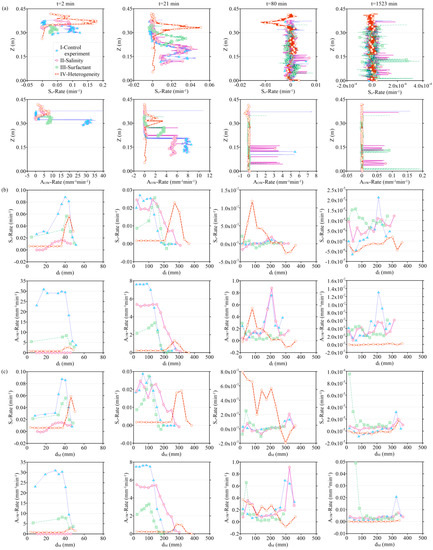
Figure 5.
(a) The change rates of PCE saturation (So) and PCE–-water interfacial area (AOW) along the sandbox profile for location x = 0.30 m; (b) tThe change of average So-rate rate and AOW-rate rate as dI increases; and (c) tThe change of average So-rate rate and AOW-rate rate as dM increases.
Mass The mass center coordinate of the PCE plume (the first moments) can be obtained based on Equations (S2) and (S3). Eventually, the change of average So-rate rate and AOW-rate rate with the distance (dI) from the injection point to the considered point in the PCE plume are presented in Figure 5b. The So-rate rate changes obviously when dI increases before t = 80 min. The AOW-rate rate decreases as dI increases at t = 21 min, while the AOW-rate rate keeps remains at a low level for Experiment-Experiment IV (heterogeneity). Simultaneously, the change of average So-rate rate and AOW-rate rate with dM (the distance from the mass center to the considered point contained in the PCE plume) is illustrated in Figure 5c. According to the results presented in Figure 5b,c, the average So-rate rate appears at a peak and then decreases with the increase of in dM and dI for all experiments at t = 2 min. The average So-rate rate decreases with increasing ofthe increase in dM and dI for all experiments at t = 21 min, while the value of the So-rate rate is very low for heterogeneous conditions (Experiment-Experiment IV). After t = 80 min, the shape of the average So-rate rate along dM and dI is very different for Experiment-Experiment IV, which suggests heterogeneity has an important effect on the distribution of the So-rate rate and AOW-rate rate along dM and dI.
3.2. The REV of So Rate and AOW Rate
The 2D sandbox domain for all experiments is discretized into 1200 cells with dimensions of 0.015 m × 0.015 m. The measured scale is increasingncreases from the center of every cell to calculate the So-rate rate and AOW-rate rate. Afterward, the corresponding ε_g^i is calculated to estimate REV based on Equation (S6). To facilitate the observation of REV estimation for characteristics of the So-rate rate and AOW-rate rate, 4 four observation cells are selected from four experiments (Figure 3a). Figure 6a,b show the change of So-rate rate and AOW-rate rate as measured size increases at t = 1523 min for observation cells selected from the four experiments. In most cases, the REV plateau delineating REV region II is not observed from the curves of the So-rate rate and AOW-rate rate, indicating that direct So-rate and AOW-rate curves areit is impossible to directly identify the REV plateau from the So rate and AOW rate curves in realistic experimental conditions. The ε_g^i calculated using Equation (S6) generally results in a more explicit REV plateau (Figure 6a,b). Erratic variation at small window size was observed for incremental growth in measured size, which is consistent with micro scales in the region I (Figure 2b). As the measured scale becomes larger, the variability and magnitude of ε_g^i decrease obviously.
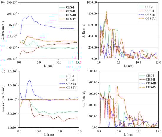
Figure 6.
(a) The change of So rate for observation cells as measured scale increases and corresponding ; (b) the change of AOW rate for observation cells as measured scale increases and corresponding .
The REVs of all cells contained in the PCE plume are estimated for all experiments. Afterward, distributions of the So-rate rate REV (SR-REV) and AOW-rate rate REV (AR-REV) of the PCE plume during the entire experimental period are presented in Figure 7a,b, respectively. Due to the large number of cells contained in the PCE plume, the statistical power is yielded by the greater number of SR-REV and AR-REV data, and the prediction based on the BP neural network is conducted. The cCorresponding results of the BP neural network for SR-REV and AR-REV are shown in Figure 8a,b.
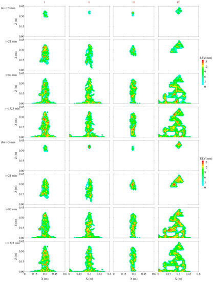
Figure 7.
The distributions of SR-REV (a) and AR-REV (b) during the entire experiment period.
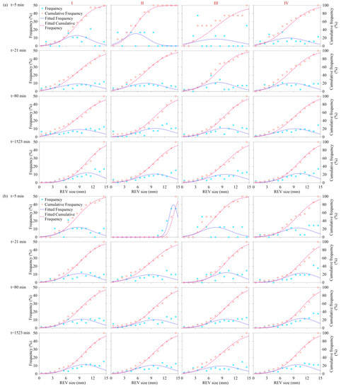
Figure 8.
The temporal change of fFrequency (histograms), cumulative frequency (solid lines) of SR-REV (a) and AR-REV (b) sizes, and associated prediction results of the BP neural network (dashed lines) are fitted during the entire experiment period for Experiments I~IV.
At the beginning of the experiment, at t = 5 min, little PCE is injected into the sandbox, and the shapes of frequency of SR-REV and AR-REV are very irregular (Figure 8a,b). As more and more PCE comes into the 2D sandbox, the PCE plume is expanded, and the frequency of SR-REV and AR-REV is changed. The results of frequency suggest SR-REV and AR-REV distribute in 3.0 mm–15.0 mm after t = 80 min. At t = 1523 min, the frequency and cumulative frequency of SR-REV and AR-REV remain at a steady state.
3.3. Predicting REV Based on BP Neural Network
The change in the average SR-REV and AR-REV as dI and dM increase is shown in Figure 9a. Regression analysis is conducted for the average SR-REV, AR-REV, and dI, dM to derive fitted models (Table S2). The average SR-REV first decreases and then increases when dI is increased for Experiments I~III. Compared with the relationship between average SR-REV and dI for Experiment I, the average SR-REVs are all reduced for Experiment II (high salinity) and Experiment IV (heterogeneity). When the concentration of the surface active agent is increased (Experiment III), the average SR-REV increases as dI increases. A similar phenomenon also appears for the relationship between the average SR-REV and dM. However, the average AR-REV shows a declining tendency as dI and dM increase for Experiment I. When the experimental condition is changed, the relationship between AR-REV and dI and dM is clearly changed, suggesting the salinity, concentration of the surface active agent, and heterogeneity have an important influence on the distribution of AR-REV for the PCE plume.
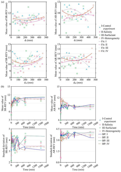
Figure 9.
(a) The change of average SR-REV and AR-REV as dI, dM increase; (b) the change of mean values and standard deviations of SR-REV and AR-REV with time.
The BP neural network is built to predict the change of the mean and standard deviation of SR-REV and AR-REV as time goes on (Figure 1b). The BP neural network contains four input layers, five hidden layers, and one output layer. The four input layers are time (tk) and the three REV values before the considered time (REVk−3, REVk−2, REVk−1); the one output layer represents the REV value at the considered time (REVk). After training, the BP neural network can be used to simulate and predict the mean and standard deviation of SR-REV and AR-REV. According to the prediction of the BP neural network, the mean and standard deviation of SR-REV remain at a steady level after t = 630 min, and the mean and standard deviation of AR-REV reach a steady state after t = 1523 min. The mean and standard deviation of SR-REV, AR-REV (point), and the predicted result based on the BP neural network (line) of the PCE plume for all experiments are presented in Figure 9b.
Simultaneously, the models are built based on the Gaussian equation to predict the frequency of SR-REV and AR-REV. The model used to predict the frequency of SR-REV and AR-REV is given by the following:
where F is the frequency of SR-REV or AR-REV; υ and δ are parameters predicted by the BP neural network. The models of the frequency of SR-REV and AR-REV are derived from the BP neural network and Gaussian equation (Tables S3 and S4). Most models can simulate the frequency and cumulative frequency of SR-REV and AR-REV with good agreement (Figure 8a,b).
It is obvious that the mean value of SR-REV is reduced under conditions of high salinity and heterogeneity, while the mean value is increased under the condition of a high concentration of the surface active agent. However, mean values of AR-REV appear to have no apparent difference under different experimental conditions. Interestingly, the standard deviation of SR-REV has a higher value under conditions of high salinity, high concentration of the surface active agent, and heterogeneity, while the standard deviation of AR-REV is not affected by these conditions. These phenomena suggest experimental conditions have a larger effect on SR-REV.
4. Conclusions
In this study, four experiments are performed to explore the effects of salinity, surface active agent, and heterogeneity on the So rate, AOW rate, and associated REV for the PCE plume. Regression analysis is utilized to derive models of the frequency of SR-REV and AR-REV and the change of REVs as dI, dM increase. Moreover, a BP neural network is built to predict the frequency of SR-REV and AR-REV. Experimental results suggest the salinity, surface active agent, and heterogeneity have an important influence on the So rate, AOW rate SR-REV, and AR-REV for PCE transport in porous media. The salinity, surface active agent, and heterogeneity lower the σz of the PCE plume. For the second moment of the PCE plume, the salinity increases σxx, while the surface active agent and heterogeneity all decrease σzz. Heterogeneity has the biggest influence on the GTP, the distribution of the So rate and AOW rate along the depth for location x = 0.30 m, and the distribution of the So rate and AOW rate along dM, dI. High salinity and heterogeneity reduce SR-REV, while the high concentration of the surface active agent increases SR-REV. The salinity, surface active agent, and heterogeneity all increase the standard deviation of SR-REV, while these factors have no apparent influence on the mean and standard deviation of AR-REV. Significantly, the frequency and cumulative frequency of SR-REV and AR-REV are predicted by the BP neural network and Gaussian equation with good agreement. These findings are significant in improving our understanding of PCE characteristics of the transport process and help to predict contaminants’ migration behavior and the associated REVs in aquifers with higher accuracy, which is the basis of the design of an effective remediation scheme for groundwater contamination.
Supplementary Materials
The following supporting information can be downloaded at: https://www.mdpi.com/article/10.3390/separations10080446/s1, Text S1: The spatial moment; Text S2: GTP analysis; Text S3: REV estimation; Table S1: Experimental conditions; Table S2: The fitted models between average REV of So rate, AOW rate and dI, dm; Table S3: The predicted frequency of SR-REV by BP neural network; Table S4: The predicted frequency of AR-REV by BP neural network. References [31,32,33,34] are cited in the supplementary materials.
Author Contributions
Z.C.: conceptualization, methodology, writing—original draft, and project administration; G.L.: conceptualization, methodology, and writing—original draft; M.W.: conceptualization, methodology, writing—review and editing, funding acquisition, and project administration; Q.L.: conceptualization, methodology. All authors have read and agreed to the published version of the manuscript.
Funding
This research was supported by the Natural Science Foundation of Guangdong Province (no. 2022A1515010273, 2023A1515012228), the Natural Science Foundation of Guangzhou City (no. 202201010414), and the National Key Research and Development Plan of China (no. 2019YFC1804302).
Data Availability Statement
Data will be made available on request.
Conflicts of Interest
The authors declare no conflict of interest.
References
- Alazaiza, M.Y.D.; Copty, N.K.; Abunada, Z. Experimental investigation of cosolvent flushing of DNAPL in double-porosity soil using light transmission visualization. J. Hydrol. 2020, 584, 124659. [Google Scholar] [CrossRef]
- Bob, M.M.; Brooks, M.C.; Mravik, S.C.; Wood, A.L. A modified light transmission visualization method for DNAPL saturation measurements in 2-D models. Adv. Water Resour. 2008, 31, 727–742. [Google Scholar] [CrossRef]
- Brown, G.O.; Hsieh, H.T. Evaluation of laboratory dolomite core sample size using representative elementary volume concepts. Water Resour. Res. 2000, 36, 1199–1207. [Google Scholar] [CrossRef]
- Chen, Y.F.; Yu, H.; Ma, H.Z.; Li, X.; Hu, R.; Yang, Z.B. Inverse modeling of saturated-unsaturated flow in site-scale fractured rocks using the continuum approach: A case study at Baihetan dam site, Southwest China. J. Hydrol. 2020, 584, 124693. [Google Scholar] [CrossRef]
- Cheng, Z.; Gao, B.; Xu, H.X.; Sun, Y.Y.; Shi, X.Q.; Wu, J.C. Effects of surface active agents on DNAPL migration and distribution in saturated porous media. Sci. Total Environ. 2016, 571, 1147–1154. [Google Scholar] [CrossRef]
- Cochennec, M.; Davarzani, H.; Davit, Y.; Colombano, S.; Ignatiadis, I.; Masselot, G.; Quintard, M. Impact of gravity and inertia on stable displacements of DNAPL in highly permeable porous media. Adv. Water Resour. 2022, 162, 104139. [Google Scholar] [CrossRef]
- Costanza-Robinson, M.S.; Estabrook, B.D.; Fouhey, D.F. Representative elementary volume estimation for porosity, moisture saturation, and air-water interfacial areas in unsaturated porous media: Data quality implication. Water Resour. Res. 2011, 47, W07513. [Google Scholar] [CrossRef]
- C’Carroll, K.; McDonald, K.; Marble, J.; Russo, A.E.; Brusseau, M.L. The impact of transitions between two-fluid and three-fluid phases on fluid configuration and fluid-fluid interfacial area in porous media. Water Resour. Res. 2015, 51, 7189–7201. [Google Scholar] [CrossRef]
- Dawson, H.E.; Roberts, P.V. Influence of viscous, gravitational, and capillary forces on DNAPL saturation. Groundwater 1997, 35, 261–269. [Google Scholar] [CrossRef]
- Ercanoglu, M. Landslide susceptibility assessment of SE Bartin (West Black Sea region Turkey) by artificial neural networks. Nat. Hazard. Earth Sys. 2005, 5, 979–992. [Google Scholar] [CrossRef]
- Filippini, M.; Parker, B.L.; Dinelli, E.; Wanner, P.; Chapman, S.W.; Gargini, A. Assessing aquitard integrity in a complex aquifer-aquitard system contaminated by chlorinated hydrocarbons. Water Res. 2020, 171, 115388. [Google Scholar] [CrossRef]
- Garcia, A.N.; Boparai, H.K.; Chowdhury, A.I.A.; Boer, C.V.D.; Kocur, C.M.D.; Passeport, E.; Lollar, B.S.; Austrins, L.M.; Herrera, J.; O’Carroll, D.M. Sulfidated nano zerovalent iron (S-nZVI) for in situ treatment of chlorinated solvents: A field study. Water Res. 2020, 174, 115594. [Google Scholar] [CrossRef]
- Gilevska, T.; Passeport, E.; Shayan, M.; Seger, E.; Lutz, E.J.; West, K.A.; Morgan, S.A.; Mack, E.E.; Lollar, B.S. Determination of in situ biodegradation rates via a novel high resolution isotopic approach in contaminated sediments. Water Res. 2019, 149, 632–639. [Google Scholar] [CrossRef] [PubMed]
- Grant, G.P.; Gerhard, J.I.; Kueper, B.H. Multidimensional validation of a numerical model for simulating a DNAPL release in heterogeneous porous media. J. Contam. Hydrol. 2007, 92, 109–128. [Google Scholar] [CrossRef] [PubMed]
- Hadley, P.W.; Newell, C. The New Potential for Understanding Groundwater Contaminant Transport. Groundwater 2014, 52, 174–186. [Google Scholar] [CrossRef] [PubMed]
- Landrigan, P.; Fuller, R.; Acosta, N.J.R.; Adeyi, O.; Arnold, R.; Basu, N.; Baldé, A.B.; Bertollini, R.; Reilly, S.B.; Boufford, J.I.; et al. The Lancet Commission on pollution and health. Lancet 2017, 391, 462–512. [Google Scholar] [CrossRef]
- Leeuwen, J.A.V.; Hartog, N.; Gerritse, J.; Gallacher, C.; Helmus, R.; Brock, O.; Parsons, J.R.; Hassanizadeh, S.M. The dissolution and microbial degradation of mobile aromatic hydrocarbons from a Pintsch gas tar DNAPL source zone. Sci. Total Environ. 2020, 722, 137797. [Google Scholar] [CrossRef]
- Li, P.J.; Zha, Y.Y.; Shi, L.S.; Tso, C.H.M.; Zhang, Y.G.; Zeng, W.Z. Comparison of the use of a physical-based model with data assimilation and machine learning methods for simulating soil water dynamics. J. Hydrol. 2020, 584, 124692. [Google Scholar] [CrossRef]
- Mo, S.; Zhu, Y.; Zabaras, N.J.; Shi, X.; Wu, J.C. Deep convolutional encoder-decoder networks for uncertainty quantification of dynamic multiphase flow in heterogeneous media. Water Resour. Res. 2019, 55, 703–728. [Google Scholar] [CrossRef]
- Niemet, M.R.; Selker, J.S. A new method for quantification of liquid saturation in 2D translucent porous media systems using light transmission. Adv. Water Resour. 2001, 24, 651–666. [Google Scholar] [CrossRef]
- Omirbekov, S.; Colombano, S.; Alamooti, A.; Batikh, A.; Cochennec, M.; Amanbek, Y.; Ahmadi-Senichault, A.; Davarzani, H. Experimental study of DNAPL displacement by a new densified polymer solution and upscaling problems of aqueous polymer flow in porous media. J. Contam. Hydrol. 2023, 252, 104120. [Google Scholar] [CrossRef] [PubMed]
- Pan, Y.; Zeng, X.K.; Xu, H.X.; Sun, Y.Y.; Wang, D.; Wu, J.C. Assessing human health risk of groundwater DNAPL contamination by quantifying the model structure uncertainty. J. Hydrol. 2020, 584, 124690. [Google Scholar] [CrossRef]
- Polykretis, C.; Ferentinou, M.; Chalkias, C. A comparative study of landslide susceptibility mapping using landslide susceptibility index and artificial neural networks in the Krios River and Krathis River catchments. B. Eng. Geol. Environ. 2014, 14, 607–613. [Google Scholar] [CrossRef]
- Schaefer, C.E.; White, E.B.; Lavorgna, G.M.; Annable, M.D. Dense nonaqueous-phase liquid architecture in fractured bedrock: Implications for treatment and plume longevity. Environ. Sci. Technol. 2016, 50, 207–213. [Google Scholar] [CrossRef] [PubMed]
- Sun, A.Y.; Scanlon, B.R.; Zhang, Z.; Walling, D.; Bhanja, S.N.; Mukherjee, A.; Zhong, Z. Combining physically based modeling and deep learning for fusing GRACE satellite data: Can we learn from mismatch? Water Resour. Res. 2019, 55, 1179–1195. [Google Scholar] [CrossRef]
- Tsai, T.T.; Kao, C.M.; Hong, A. Treatment of tetrachloroethylene-contaminated groundwater by surfactant-enhanced persulfate/BOF slag oxidation- A laboratory feasibility study. J. Hazard Mater. 2009, 171, 571–576. [Google Scholar] [CrossRef]
- Wang, Y.; Bian, J.; Sun, X.; Ruan, D.; Gu, Z. Sensitivity-dependent dynamic searching approach coupling multi-intelligent surrogates in homotopy mechanism for groundwater DNAPL-source inversion. J. Contam. Hydrol. 2023, 255, 104151. [Google Scholar] [CrossRef]
- Weisbrod, N.; Niemet, M.R.; Selker, J.S. Light transmission technique for the evaluation of colloidal transport and dynamics in porous media. Environ. Sci. Technol. 2003, 37, 3694–3700. [Google Scholar] [CrossRef]
- Wu, M.; Wu, J.F.; Wu, J.C. Simulation of DNAPL migration in heterogeneous translucent porous media based on estimation of representative elementary volume. J. Hydrol. 2017, 553, 276–288. [Google Scholar] [CrossRef]
- Zhou, Z.K.; Shi, L.S.; Zha, Y.Y. Seeing macro-dispersivity from hydraulic conductivity field with convolutional neural network. Adv. Water Resour. 2020, 138, 103545. [Google Scholar] [CrossRef]
- Christ, J.A.; Ramsburg, C.A.; Pennell, K.D.; Abriola, L.M. Estimating mass discharge from dense nonaqueous phase liquid source zones using upscaled mass transfer coefficients: An evaluation using multiphase numerical simulations. Water Resour. Res. 2006, 42, W11420. [Google Scholar] [CrossRef]
- Natarajan, N.; Kumar, G.S. Spatial moment analysis of multispecies contaminant transport in porous media. Environ. Eng. Res. 2018, 23, 76–83. [Google Scholar] [CrossRef]
- Wu, M.; Wu, J.F.; Wu, J.C.; Hu, B.X. A new criterion for determining the representative elementary volume of translucent porous media and inner contaminant. Hydrol. Earth Syst. Sci. 2020, 24, 5903–5917. [Google Scholar] [CrossRef]
- Zheng, F.; Gao, Y.W.; Sun, Y.Y.; Shi, X.Q.; Xu, H.X.; Wu, J.C. Influence of flowvelocity and spatial heterogeneity on DNAPL migration in porous media: Insightsfrom laboratory experiments and numerical modeling. Hydrogeol. J. 2015, 23, 1703. [Google Scholar] [CrossRef]


Disclaimer/Publisher’s Note: The statements, opinions and data contained in all publications are solely those of the individual author(s) and contributor(s) and not of MDPI and/or the editor(s). MDPI and/or the editor(s) disclaim responsibility for any injury to people or property resulting from any ideas, methods, instructions or products referred to in the content. |
© 2023 by the authors. Licensee MDPI, Basel, Switzerland. This article is an open access article distributed under the terms and conditions of the Creative Commons Attribution (CC BY) license (https://creativecommons.org/licenses/by/4.0/).