A Fault Identification Method in Distillation Process Based on Dynamic Mechanism Analysis and Signed Directed Graph

Abstract

Due to the complexity of materials and energy cycles, the distillation system has numerous working conditions difficult to troubleshoot in time. To address the problem, a novel DMA-SDG fault identification method that combines dynamic mechanism analysis based on process simulation and signed directed graph is proposed for the distillation process. Firstly, dynamic simulation is employed to build a mechanism model to provide the potential relationships between variables. Secondly, sensitivity analysis and dynamic mechanism analysis in process simulation are introduced to the SDG model to improve the completeness of this model based on expert knowledge. Finally, a quantitative analysis based on complex network theory is used to select the most important nodes in SDG model for identifying the severe malfunctions. The application of DMA-SDG method in a benzene-toluene-xylene (BTX) hydrogenation prefractionation system shows sound fault identification performance.

1. Introduction

Distillation is one of the most important parts of chemical production. Doubtlessly, its smooth operation is crucial to the safety of the entire chemical plant. Due to strong coupling of process variables, high sensitivity, complex operation, and difficulty in direct control of key variables such as temperature and pressure, distillation is more prone to failure than other unit operations. A slight deviation of the complex separation system variable can be a trigger to a chain reaction in the system, resulting in the loss of efficiency and reliability [1]. Once the system is out of control, extremely high pressure and flammable materials may cause material loss and human casualties, even an explosion in the distillation column [2]. Therefore, how to accurately identify the faults in the distillation system has become a key issue to ensure safe production in chemical industry.

However, in the actual production process, there are some difficulties in the analysis and research of faults. Faults that cause serious damage to the distillation system are the “black swan” incidents, which are not only almost unpredictable, but also serious in consequences. In addition, it is difficult to detect slight deviations of process variables and changes in the external environment in the course of operation [3]. To address the above problems, process simulation is introduced in this paper to provide data and mechanism support for fault analysis. As a multipurpose and maneuverable process simulation method, dynamic simulation is able to accurately reflect the timely response of chemical processes by introducing time variables [4]. Dynamic simulation is frequently used as a substitute for real situation to optimize process system, demonstrate the complex control system scheme, and observe the dynamic changes of the system when faults occur [5]. For instance, dynamic simulation made a great contribution to the proposal of an effective control scheme for the coal pyrolysis wastewater treatment process [6]. A rigorous distillation model with explicit heat-exchanger dynamics in dynamic simulation was used for safety analysis under emergency [7]. The SIL (safety integrity level) analysis of a fractionating system with the grade of control schemes referenced to the importance rank of process variables was completed based on dynamic simulation [8]. Dynamic simulation also played a key role in providing quantitative variable deviations into hazard and operability analysis (HAZOP) to guide the design of control structure for the whole plant [9]. Variable deviation scenarios of dynamic simulation for benzene alkylation process were analyzed to explore the deviation propagation effects and make contribution to the quantitative risk assessment (QRA) [10]. A robust fault detection method for the distillation column was effectively verified by setting and analyzing the fault types in dynamic simulation [11]. Dynamic simulation provided a data set, at normal and faulty states, for the fault classification of multikernel support vector machines [12]. A quantitative HAZOP method with dynamic simulation as a deviation reasoning tool was developed to reduce uncertainty in manual HAZOP analysis [13].

At present, fault detection and identification (FDI) methods mainly include analytical model-based methods, data-driven methods, and knowledge-based methods [14]. The application of analytical model-based methods have obvious limitations due to the uncertainty for the complex interrelationship of variables and the mechanism of some reaction processes. Currently, research on data-driven methods such as a series of supervised machine learning has also stagnated. Since the recognition effect of supervised deep learning depends largely on the labeling preprocessing of training dataset, a new type of fault that has never been learned by the deep learning model is difficult to identify. Compared to the above two methods, knowledge-based methods not only avoid the establishment of complex mechanism simulation models, but also provide a reasonable explanation for the complex variable relationships in the system by empirical knowledge [15]. A case-based reasoning method combining a case simplification method and a case reuse strategy was proposed to reduce the time lag and complexity of fault identification and improve the accuracy of fault diagnosis results [16]. A hybrid safety performance evaluation framework for offshore oil and gas platforms was built, which uses safety score of system to guide the selection of fuzzy expert systems [17]. Among the many knowledge-based FDI methods, the signed directed graph (SDG) is a graphical model that vividly reflects the system structure and the correlation among variables in the process. An integrated fault diagnosis framework combining fuzzy logic-based SDG and reconstruction-based multivariate contribution analysis (RBMCA) was established to identify the root cause of the detected fault without historical data of known fault types [18]. An alarm signal screening method based on the probability SDG was proposed, which effectively reduces the missed alarm and false alarm probabilities [19]. By integrating multilevel flow modeling (MFM) and SDG, a functional modeling method of fault diagnosis systems was designed to address the difficulties regarding the interpretation of results and consistent graph generation [20]. A graphic construction methodology that builds the SDG directly from a bond graph was proposed to reduce modeling complexity [21]. A new method was presented to improve the resolution of fault identification, which integrates the completeness feature of SDG with the good diagnostic resolution feature of qualitative trend analysis (QTA) [22]. The above references all show that SDG, as a qualitative FDI method, can identify faults without the need of historical data but reflect the essential mechanism of the process.

This paper proposes a fault identification method for the distillation process, combining dynamic mechanism analysis with an SDG model (DMA-SDG). The DMA-SDG method establishes a dynamic model to offer the mechanism analysis for the process, and then characterizes fault feature by deviation propagation paths. The outline of this paper is organized as follows. In Section 2, the framework of the DMA-SDG method is introduced in detail, followed by the principles of process simulation and SDG. The excellent performance of the DMA-SDG method is proved by a case study in the Section 3. The final section gives the conclusions by summarizing the highlights of the proposed method.

2. Proposed Method

The framework of DMA-SDG method is shown in Figure 1. The specific innovations are as follows:

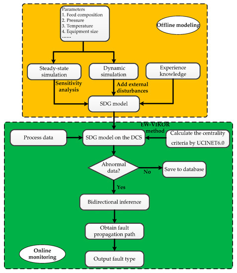
Figure 1. The framework of the dynamic mechanism analysis and signed directed graph (DMA-SDG) method.

• A steady-state simulation is established based on the data parameters of the distillation process. The dynamic simulation with effective control schemes is built according to the steady-state simulation. Dynamic mechanism analysis is applied by combining quantitative dynamic response with expert knowledge. SDG models are constructed by connecting process variables with positive and negative feedback relationships.
• The SDG model is connected to the distributed control system (DCS) for process monitoring. For abnormal process data, the SDG model can accurately describe the fault feature as the consistent path by bidirectional inference. Then, the fault type marked with the feature is outputted and displayed to the operators.
• The nodes in the SDG model are ranked in importance using the entropy weighting (EW)-VIKOR method, a method to evaluate node importance in complex network [23] by UCINET6.6. Faults related to important nodes that have a severe harm to the distillation system are marked and analyzed.

2.1. Dynamic Mechanism Analysis Based on Process Simulation

A steady-state simulation is a quantitative calculation of the characteristic equations in a chemical process. The data of the chemical process involved in the simulation includes the temperature, pressure, flow rate, composition of the feed, relevant process operating conditions, process regulations, and equipment parameters. However, there is no time variable in steady-state simulation, which is not consistent with the actual process system. In order to solve this defect, dynamic simulation is introduced to study dynamic phenomena of complex chemical process.

The remarkable feature of dynamic simulation is the ability to use proportion integral differential (PID) for process variable control and optimization of system operation. The structure of a typical PID controller based on feedback control is shown in Figure 2.

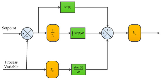
Figure 2. Schematic diagram of the typical proportion integral differential (PID) controller.

A PID controller consists of proportional control, integral control, and differential control. The proportional control, which is denoted as err(t), reflects the error signal of the control system proportionally and generates an immediate control action to reduce the deviation once it occurs. The integral control, which is denoted as ∫err(t)dt, mainly eliminates static errors to improve the indiscrimination degree of the system. The differential control, which is denoted as derr(t)/dt, reflects the trend of the errors and responds early before the errors become too large, thus speeding up the system action.

The PID controller based on feedback control is introduced as follows. The process variable is measured and compared with its set point, and then the obtained error is fed back to the controller. The controller determines the output value according to the error and the control algorithm. The control valve is executed under the guidance of the output value to adjust the process variable near the set point. The calculation formula of PID is given in Equation (1):

$$U(t)=k_p(err(t)+\frac{1}{T_I}{\displaystyle \int err(t)dt+}{T}_D\frac{derr(t)}{dt})$$

(1)

where U(t) is the output value of controller, err is the gap between the setpoint and the process variable, err(t) is the part of proportional control, ∫err(t)dt is the part of proportional control, derr(t)/dt is the part of proportional control, and k_p, 1/T_I, T_D are the corresponding coefficients.

Due to the immense amount of operating parameters in the chemical processes, a qualitative and static analysis alone cannot meet the requirements of a process-specific analysis. To better incorporate mechanism knowledge and refine the SDG modeling, dynamic mechanism analysis based on dynamic simulation is proposed in this paper. In this method, deviations sufficient to cause the system faults are given by changing parameters in dynamic simulation. By dynamic simulation with the PIDs, the initial variable deviations are dynamically responded by the automatic control of the controllers based on the material and energy flow within the devices. The propagation paths of the deviations are quantitatively depicted in the dynamic simulations, in which the expert knowledge is added to provide a mechanistic explanation of the deviation relationships among variables.

2.2. Signed Directed Graph

2.2.1. SDG Model

SDG is a qualitative analysis graph that expresses the mutual influence among process variables. It reflects the characteristics of the devices involved and the overall topology of the system. The determination of the directed arcs between nodes is conducive to fully reveal the fault propagation relationship among process variables. Based on the bidirectional inference method and the principle of information compatibility, SDG can be employed to reveal the internal causality of complex systems and explain the occurrence and spread of accidents.

A SDG model is a network diagram consisting of nodes and directed arcs connecting them. A simple example of a SDG model is shown in Figure 3. Nodes in the SDG model can be the physical variables such as pressure and temperature in the system, or operating variables such as valves and controllers. The states of the node are “+”, “0” or “−”, which represent greater than the upper threshold, normal state and less than the lower threshold respectively. The nodes are connected by directed arcs, indicating the influence relationship between them. The situation that the trend of two nodes is the same, which means an increase in the former node leading to an increase in the latter node, is generally represented by a solid arrow connecting the two nodes. Conversely, when two nodes are trending in opposite directions, that is, an increase in the previous node leads to a decrease in the following node, dashed arrows are placed to connect the two nodes. In Figure 3, the states of A, B and C are “+”, “+”and “−” respectively. The relationship between A and B is denoted by a solid arrow, and the one between B and C is denoted by a dashed arrow. This means that an increase in A leads to an increase in B, and then leads to a decrease in C.

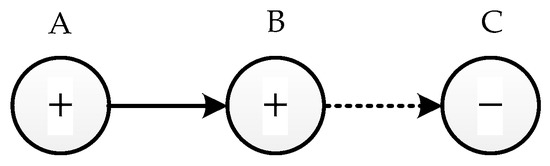
Figure 3. A simple SDG model structure.

Moreover, SDG can be described mathematically in a rigorous way [24]. The SDG model γ is a combination of the set of directed graphs G and the set of functions φ, which can be denoted as Equation (2). The set of directed graphs G, given as Equation (3), consists of three parts, the set of nodes V = {v_i}, the set of arcs E = {e_k} and the adjacent associates δ⁺: E→V and δ⁻: V→E, where the adjacency associates δ⁺: E→V and δ⁻: V→E are the origin nodes δ⁺e_k and end nodes δ⁻e_k of the arc e_k, respectively. The arc e_k is noted as Equation (4), meaning the directed arc from v_i to v_j. And the set of functions φ is denoted as Equation (5), indicating that φ is the sign of arc e_k and is taken the values “+” or “−”:

$$\gamma =\left(G,\phi \right)$$

(2)

$$G=(V,E,{\delta }^{+},{\delta }^{-})$$

(3)

$$e_k=\left(v_i,v_j\right)\in E$$

(4)

$$E\to \left\{+,-\right\}, \phi \left(e_k\right)=\phi \left(v_i,v_j\right)$$

(5)

The sample of the SDG model γ corresponds to a function ψ of the node state values, as given in Equation (6). The symbol for node v_i is noted as ψ(v_i), which has three values, as shown in Equations (7)–(9):

$$\psi :V\to \left\{+,0,-\right\}$$

(6)

$$\psi \left(v_i=+\right)\hspace{1em}\left(X{v}_i-\overline{X}{v}_i\ge \epsilon v_i\right)$$

(7)

$$\psi \left(v_i=0\right)\hspace{1em}\left(\left|X{v}_i-\overline{X}{v}_i\right|\le \epsilon v_i\right)$$

(8)

$$\psi \left(v_i=-\right)\hspace{1em}\left(X{v}_i-\overline{X}{v}_i\le \epsilon v_i\right)$$

(9)

where Xv_i is the measured value of node v_i, $\overline{X}$v_i is the value of node v_i in the steady state of the system, and εv_i is the threshold value of node v_i in the normal state. For ease of representation, the upper and lower thresholds of the node are both denoted by εv_i, and in practice they are set on a case-by-case basis.

When fault identification is performed by the SDG model, the arc e_k whose state satisfies Equation (10) is called the consistent arc. The set of all consistent arcs are called the consistent path which represents the pathway propagated within the SDG model:

$$\psi ({\delta }^{+}{e}_k)\phi \left(e_k\right)\psi ({\delta }^{-}{e}_k)=+$$

(10)

2.2.2. Fault Identification Based on SDG Model

An efficient fault inference algorithm is the basis for the efficient operation of the fault identification method based on SDG. Inverse inference is the traditional inference method for the SDG model, which main contents are illustrated as follows. When an alarm occurs, the instantaneous statuses of all nodes in SDG model are determined by comparing them with a predefined threshold value. Then, from the node where the first abnormal state appears, inverse search is performed in the direction opposite to the arcs until the nodes that cause the alarm is found. When the search proceeds on current node, the consistency of the arc to it should be fulfilled, as shown in Equation (10). If Equation (10) is confirmed in this search arc, the current node is marked as a cause node, and the search arc becomes the consistent arc. The search is repeated until all abnormal nodes are found and all the identified consistent arcs are combined into the consistent path.

Due to the multitude of assumptions made in the modeling process, inverse inference is often carried out to reason many cause nodes under complex systems. The resolution and operational speed of fault identification method are thus severely impaired by a large volume of nodes. In this paper, a more effective bidirectional inference algorithm is adopted to ensure the validity of the fault identification results. Bidirectional inference integrates inverse inference based on inductive method and forward inference based on deductive method. Primarily, all possible fault cause nodes are searched using inverse inference mentioned above, and then forward inference is performed for each of them in turn to verify the veracity. The detailed steps of bidirectional inference are shown in Figure 4.

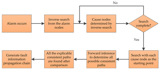
Figure 4. The flow chart of bidirectional inference.

To illustrate the principle of SDG more clearly, a liquid level control system and its SDG model are shown in Figure 5 as an example. In Figure 5, the level control system consists of two tanks and a centrifugal pump primarily, which entirely relies on a level controller to alleviate external disturbances. The inlet and outlet flow rates of the whole process F1 and F3 are controlled by the valves V1 and V3 respectively. The liquid in Tank 1 is transported by gravity to Tank 2 where a level controller LIC is installed to stabilize its level by regulating F2, the outlet flow rate of Tank 1. The liquid in Tank 2 is transported out of this system by a centrifugal pump K, and the pressure of this stream is monitored by a pressure monitor P. L and V2 are the level of Tank 1 and the valves controlled by the LIC on stream F2.

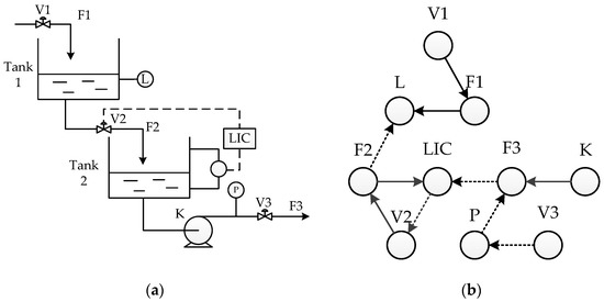
Figure 5. Schematic diagram of the liquid level control system and its SDG model: (a) liquid level control system; (b) SDG model of liquid level control system.

Assuming that the overopening of V3 results an alarm of node L, the bidirectional inference method is carried out. First, the state of L is detected to be below the threshold value. By inverse inference the consistent path is obtained as L(−) ←F2(+) ←V2(+) ←LIC(−) ←F3(+) ←P(−) ←V3(+).Then, forward inference from the cause node V3 is performed with consistent path. The final two inference results are consistent, and this discovered pathway is the correct consistent path. In this fault situation, the consistent path in the SDG model is shown in Figure 6. The cause node, a rectangle with the letter “R”, is introduced into the SDG model, meaning that the fault causes an offset in node V3 and further affects the system.

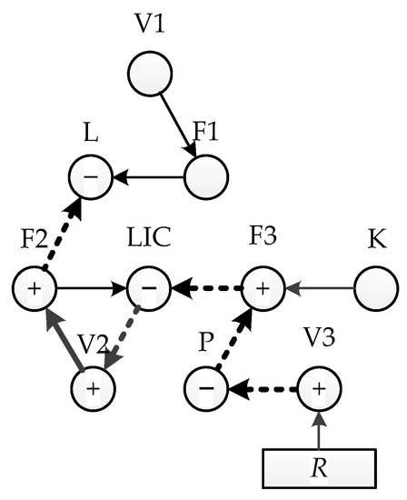
Figure 6. Consistent path in the SDG model.

3. Case Study

To verify the performance of the DMA-SDG method, it was applied to the BTX aromatics of a hydrogenation prefractionation system. This system is a very important part of the petrochemical system, which involves many flammable and explosive chemicals as the front part of the entire aromatics hydrogenation production process. Once a fault occurs, there may be overtemperature and overpressure destruction of the equipment. Dangerous materials may leak from the equipment to the outside environment, causing fire and severe explosion. Therefore, the fault identification of hydrogenation prefractionation system is particularly necessary.

In order to ensure the accuracy of the process simulation, all equipment parameters including equipment size, tray number, tray pressure drop and all operating parameters including reflux ratio, feed flow, tower top temperature and pressure are offered by a petrochemical enterprise. The reference documents obtained include a piping and instrument diagram (PI&D), a process flow diagram (PFD), DCS screenshots with operating parameters, operating manuals, etc.

3.1. Process Simulation

The flow chart of hydrogenation prefractionation is shown in Figure 7. The purpose of this process is to separate the C₅ and C₉ components in the BTX aromatics feed with two steps and then the remaining purified BTX component (benzene, toluene, xylene, etc.) is fed to the reactor for hydrogenation.

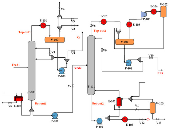
Figure 7. The flow chart of hydrogenation prefractionation system.

3.1.1. Steady-State Simulation

The steady-state simulation is established based on Figure 7. The simulation mainly uses FSplit, Heater, HeatX, Flash2 and RadFrac modules to refine the BTX aromatic components. The simulation results of major streams are listed in Table 1. In addition, the temperature profiles of the two columns are shown in Figure 8.

Table 1. Actual data and simulation result of hydrogenation prefractionation system.

Stream	Pressure (MPa)			Temperature (°C)			Mass Flows (kg/h)
	Simulation Value	Real Value	Relative Error %	Simulation Value	Real Value	Relative Error %	Simulation Value	Real Value	Relative Error %
Feed	0.2340	0.2340	0	40.08	40.1	−0.05	12,220.0	12,220.0	0.00
Feed2	0.0372	0.0372	0	115.33	115.33	0.00	9388.7	9359.6	0.31
C5	0.2093	0.2093	0	50.51	51.28	0.44	2831.3	2860.4	−1.01
BTX	0.0353	0.0353	0	46.95	47.00	−0.11	7272.9	7312.1	−0.54
C9	0.0644	0.0644	0	50.01	50.10	−0.18	2115.8	2076.6	1.89

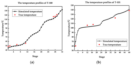
Figure 8. The temperature profiles of T-100 and T-101: (a) temperature profiles of T-100; (b) temperature profiles of T-101.

It can be seen from Table 1 that the results of the steady-state simulation are very close to the actual process data offered by the petrochemical enterprise. Figure 8a is the temperature profile for T-100, a depentanizer with a total of 32 stages and Figure 8b is the temperature profile for T-101, a distillation column with a total of 48 stages with a total of 48 stages. The temperature control stages in the actual process are stage 29 in T-100 and stage 12 and stage 35 in T-101. According to the selection method of the temperature control stages [25], the temperature control stages are selected as stage 31 in T-100 and stage 14 and stage 34 in T-101 by the slope criterion and the minimum product fluctuation criterion, which are basically same as the actual process. In addition, the tower top temperature control loop in T-100 is designed to regulate the vapor phase outlet temperature to control the return flow rate by PID. Therefore, a design consistent with the actual situation was used in the simulation. This accurate steady-state simulation lays a very solid foundation for the successful establishment of the subsequent dynamic simulation.

3.1.2. Dynamic Simulation

In this section, the controllers are installed in the dynamic simulation. The flowsheet of dynamic simulation is shown in Figure 9. This simulation system is fitted with 13 controllers, including pressure controllers, temperature controllers and liquid level controllers. These controllers are set up with reference to the control loops that have been set up in the actual process. Then they are activated to enhance the robustness of the dynamic model when external disturbances are added. In this paper, their another role is to cooperate with the device module to simulate various fault types.

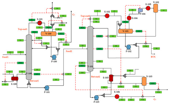
Figure 9. The flowsheet of dynamic simulation.

The main variables in the process are listed in Table 2, which can be monitored and displayed by the actual DCS system. There is a total of 54 variables including measured variables and operating variables.

Table 2. The main variables in a hydrogenation prefractionation system.

Variables	Symbol Description	Variables	Symbol Description
F1	Feed1 flow	TC3	The 14th tray temperature in T-101
F2	T-100 top reflux flow	TC4	The 34th tray temperature in T-101
F3	V-100 vapor outlet flow	L1	V-102 level
F4	C5 outlet flow	LC1	V-100 level
F5	Feed2 flow	LC2	T-100 level
F6	E-100 steam feed flow	LC3	V-101 level
F7	T-101 top outlet flow	LC4	T-101 level
F8	T-101 top reflux flow	LC5	V-103 level
F9	BTX output flow	P1	T-100 bottom pressure
F10	E-103 steam feed flow	P2	T-101 bottom pressure
F11	E-102 hot stream outlet flow	PC1	T-100 top pressure
F12	T-101 bottom reflux flow	PC2	V-100 pressure
F13	C9 outlet flow	PC3	T-101 top pressure
T1	Feed1 temperature	PC4	V-101 pressure
T2	The eighth tray temperature of T-100	V1	T-100 top reflux flow valve opening
T3	E-101 outlet temperature	V2	V-100 outlet gas flow valve opening
T4	T-100 bottom reflux temperature	V3	Nitrogen flow valve opening
T5	Feed2 temperature	V4	fixed gas flow valve opening
T6	T-101 top outlet temperature	V5	C5 output flow valve opening
T7	E-102 outlet temperature	V6	E-100 condensate flow valve opening
T8	P-104 inlet temperature	V7	Feed2 flow valve opening
T9	The 60th tray temperature in T-101	V8	T-101 top output flow valve opening
T10	T-101 bottom outlet temperature	V9	T-101 top reflux flow valve opening
T11	C9 outlet temperature	V10	BTX output flow valve opening
T12	T-101 bottom reflux temperature	V11	E-103 hot stream flow valve opening
TC1	T-100 top outlet temperature	V12	C9 output flow valve opening
TC2	The 31th tray temperature in T-100	V13	V-103 condensate flow valve opening

3.2. Establishment of SDG Model

The SDG model built based on expert knowledge [26] is tidy and streamlined for good performance for fault identification. When applying this method to build a SDG model, the determination of nodes and arcs can be conducive to the impact of the faults on the devices accurately and the paths of fault propagation. However, the performance of the model based on expert knowledge is deeply subject to the ability of the modeler. To mitigate the human impact, process simulation is introduced into the modeling process of SDG. The internal mechanism and explicit process data in process simulation are employed to analyze the relationship among process variables. The sensitivity analysis module in Aspen Plus is a useful tool to examine how manipulated variables and sampled variables affect process simulation. In this paper, this module is used to check the influence relationships among process variables. But, the application of sensitivity analysis in SDG is limited because the definition of operating variables makes it difficult for the process to converge. The sensitivity analysis in steady-state simulation is incapable of embodying the dynamic changes of variables. For a more comprehensive analysis of the relationship among process variables, external disturbances are therefore added to observe the dynamic response in the hydrogenation pre-fractionation system with controllers in the dynamic simulation.

The change of the column top temperature T6 and column bottom temperature T10 after increasing the feed temperature T5 by 10% at 2 h is shown in Figure 10. It indicates that at the beginning of the disturbance addition, T6 and T10 are rapidly vibrating. But their subsequent trends are relatively stable. The increase in feed temperature is essentially a decrease in the liquefaction fraction of the feed. In the xy phase diagram, the space between the operation line and the phase equilibrium line becomes smaller, that is, the separation space in distillation column becomes smaller. Due to the separation performance degradation of the distillation column, the heavy components in the stream Top-out2 and the light components in the stream Bot-out2 both increase. The changes of the three key components in the stream Top-out and Bot-out are shown in Figure 11. It can be seen that the mole fraction of ortho-xylene which is the light key component in the stream Top-out2 decreases gradually after the occurrence of disturbance. The mole fraction of the heavy key component para-methyl ethylbenzene in stream Bot-out2 decreases, while the mole fraction of the light key component ortho-xylene increases. The manifestation of this phenomenon on temperature changes is that T6 gradually increases and T10 gradually decreases. Based on the above analysis, the relationship among T5, T6 and T10 is determined, that is, T5 has a positive effect on T6 and a negative effect on T10.

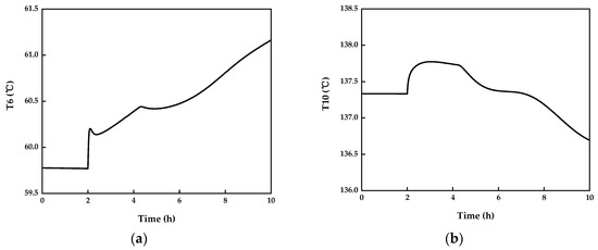
Figure 10. Effect of feed temperature T5 disturbance at 2 h on system: (a) the column top temperature T6; (b) the column bottom temperature T10.

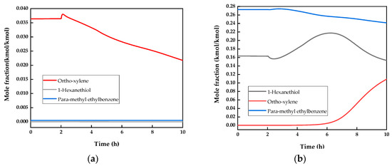
Figure 11. Three key components in stream: (a) Top-out2; (b) Bot-out2.

All relationships of node variables in the hydrogenation prefractionation system are analyzed by mechanism and process data similarly. Moreover, the listed influence relationships are combined into a complete SDG model. The obtained SDG model of the hydrogenation prefractionation system is shown in Figure 12. All nodes are connected by solid arrows or dotted arrows, which mean the positive or negative correlation among variables. To retain the most accurate features of the faults, the SDG model is appropriately simplified by reducing unnecessary arcs.

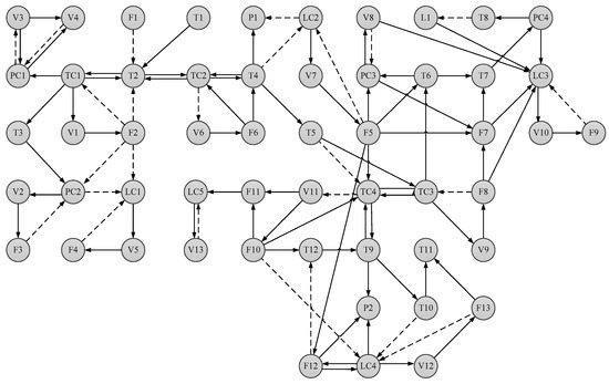
Figure 12. SDG of hydrogenation prefractionation system.

3.3. Fault Identification

In this section, the nodes importance of SDG are evaluated using the EW-VIKOR method to mark faults that cause serious damage to the hydrogenation prefractionation system. To verify the model, a fault case which refers to the evaluation of the importance of variables is set up in dynamic simulation. Finally, the consistency of the manifestations of the fault in the two models is explored, and the representation of the fault in SDG model is output as the fault feature.

3.3.1. Selection of Key Nodes in SDG Model

It is extremely difficult to list fault types one by one by exhaustive method due to the strong coupling of complex chemical engineering systems and the large number of process variables. Therefore, the complex network theory is introduced into the SDG model by the EW-VIKOR method [23] to find the nodes that are critical to the system. According to the ranking rule of node importance, the fault type that is greatly harmful to the hydrogenation prefractionation system and is closely related to important nodes can be found.

The EW-VIKOR method is a combination of entropy weighting method and VIKOR method to rank the importance of nodes in complex networks. The VIKOR method is performed to integrate multiscale centrality criteria like DC (degree centrality), BC (betweenness centrality), CC (closeness centrality), EC (eigenvector centrality), and the entropy weighting method is employed to attach the weight to the centrality criteria, reducing the human impact. Before using this method, the centrality criteria of the SDG model needs to be calculated. The calculation formulas of DC, CC, BC, and EC are defined in Equations (11)–(14), where k_i represents the number of neighbor nodes of node i, n represents the total number of nodes in SDG, d_ij represents the length for the shortest path between nodes i and j, g_jk is the total number of all shortest paths between node j and node k, g_jk(i) is the number of shortest paths between node j and node k that go through node i, n(n − 1)/2 is used as denominator to normalize the BC value, and λ is the maximum characteristic value of the adjacent matrix A. The graphic data in SDG is then abstracted into tabular data for UCINET6.6 to calculate the centrality criteria:

$${\mathrm{DC}}_i=\frac{k_i}{n-1},$$

(11)

$${\mathrm{CC}}_i=n-1/{\displaystyle \sum _{j=1}^n{d}_{ij}},$$

(12)

$${\mathrm{BC}}_i={\displaystyle \sum _{j,k\ne i}^n\frac{g_{jk}(i)}{g_{jk}}}/\frac{n(n-1)}{2}$$

(13)

$${\mathrm{EC}}_i={\lambda }^{-1}{\displaystyle \sum _{j=1}^n{a}_{ij}{x}_j}$$

(14)

Four centrality criteria are calculated by Equations (11)–(14) as the initial data of EW-VIKOR method. The importance of nodes is ranked by EW-VIKOR method through five steps. Firstly, the decision matrix D is constituted (see Equation (15)) and normalized (see Equation (16)). And the normalized decision matrix can be obtained as R = (r_ij)32 × 4. In Equation (16), the centrality criteria vector is expressed as C = [c₁, c₂, c₃, c₄], which covers DC, CC, BC and EC, the node vector is denoted as V = [v₁, v₂, …, v₃₂]^T, and v_i(c_j) represents the value of the jth criterion for the ith node:

$$\mathbf{D}=\left[\begin{array}{cccc}{v}_1(c_1)& v_1(c_2)& \cdots & v_1(c_4)\\ v_2(c_1)& v_2(c_2)& ⋮& v_2(c_4)\\ ⋮& ⋮& \ddots & ⋮\\ v_{32}(c_1)& v_{32}(c_2)& \dots & v_{32}(c_4)\end{array}\right]$$

(15)

$$r_{ij}=v_i(c_j)/\sqrt{{\displaystyle \sum _{k=1}^n{(v_k(c_j))}^2}}$$

(16)

Secondly, the weight of each criterion is calculated by the entropy weighting method. The information entropy of the jth criterion is first denoted as Equations (17) and (18), and then the weight of the jth criterion is calculated as Equation (19). In Equation (18), if r′_ij = 0, then r′_ij ln r′_ij = 0:

$${r^{\prime }}_{ij}=\frac{r_{ij}}{{\displaystyle {\sum }_{k=1}^n{r}_{kj}}}$$

(17)

$${\mathbf{E}}_j=-\frac{1}{\ln n}{\displaystyle \sum _{i=1}^n{r^{\prime }}_{ij}}\ln {r^{\prime }}_{ij}$$

(18)

$$w_j=\frac{1-{\mathrm{E}}_j}{{\displaystyle {\sum }_{k=1}^m(1-{\mathrm{E}}_k)}}$$

(19)

Thirdly, the positive solution r⁺ and the negative solution r⁻ can be determined based on the normalized decision matrix R, see Equations (20) and (21), where J and J′ are the sets of benefit criteria (the higher the criterion, the more important the node is) and cost criteria (the higher the criterion, the less important the node is), respectively. The four criteria are all benefit criteria.

$$r_j^{+}=\left\{(\underset{i}{\max }{r}_{ij}|j\in J)\mathrm{or}(\underset{i}{\min }{r}_{ij}|j\in J^{\prime })\right\}$$

(20)

$$r_j^{-}=\left\{(\underset{i}{\min }{r}_{ij}|j\in J)\mathrm{or}(\underset{i}{\max }{r}_{ij}|j\in J^{\prime })\right\}$$

(21)

Then, the utility measure S_i and the regret measure R_i for all nodes are calculated by Equations (22) and (23).

$${\mathrm{S}}_i={\displaystyle \sum _{j=1}^m{w}_j(r_j^{+}-r_{ij})/(r_j^{+}-r_j^{-})}$$

(22)

$${\mathrm{R}}_i=\underset{j}{\max }\left[w_j(r_j^{+}-r_{ij})/(r_j^{+}-r_j^{-})\right]$$

(23)

Finally, according to the utility measure S_i and the regret measure R_i, the VIKOR index for nodes can be calculated as Equation (24), where v and 1 − v are the weight of maximum group utility and the individual regret, respectively, here v = 0.5. Additionally, S* and R* are the minimum of S_i and R_i, and S⁻and R⁻ are the maximum of S_i and R_i. The lower a Q_i value is, the more important the ith node is. Table 3 lists the calculated Q_i and the ranking result for all nodes.

$${\mathrm{Q}}_i=v({\mathrm{S}}_i-{\mathrm{S}}^{\ast })/({\mathrm{S}}^{-}-{\mathrm{S}}^{\ast })+(1-v)({\mathrm{R}}_i-{\mathrm{R}}^{\ast })/({\mathrm{R}}^{-}-{\mathrm{R}}^{\ast })$$

(24)

Table 3. The ranking result of all nodes.

Rank	Node	Qi	Rank	Node	Qi	Rank	Node	Qi
1	TC4	5.62 × 10−16	19	T7	0.757596	37	V12	0.925076
2	T5	0.11938	20	V7	0.765949	38	T11	0.929671
3	F5	0.181683	21	F11	0.768166	39	F6	0.944618
4	F8	0.242207	22	T10	0.77906	40	T8	0.951836
5	PC2	0.242213	23	T4	0.790817	41	P1	0.965024
6	LC3	0.405469	24	LC2	0.803766	42	T3	0.965285
7	LC4	0.415517	25	LC1	0.804402	43	V6	0.968172
8	TC2	0.437325	26	PC1	0.813759	44	F13	0.980322
9	TC3	0.503178	27	PC4	0.821318	45	V1	0.981665
10	F7	0.514134	28	F10	0.822773	46	F9	0.989015
11	T9	0.579063	29	V10	0.851761	47	F4	0.993863
12	T6	0.609504	30	P2	0.872967	48	V5	0.993863
13	V11	0.624336	31	V8	0.878502	49	V3	0.994151
14	F12	0.633763	32	T12	0.881528	50	V4	0.994151
15	F2	0.639496	33	V9	0.884014	51	F1	0.999061
16	TC1	0.678051	34	LC5	0.894367	52	T1	0.999061
17	PC3	0.681567	35	L1	0.904892	53	V13	1
18	T2	0.686053	36	V2	0.907141	54	F3	1.003796

As can be seen in Table 3, among the 54 variables, the first eight most important nodes with low Q_i values for the network are TC4, T5, F5, F8, PC2, LC3, LC4 and TC2. This ranking result is consistent with the results of the mechanism and process data analysis. For example, TC2 and TC4 can represent the key points on the temperature profile in T-100 and T-101, which are the temperature of sensitive stages (31th tray in T-100 and 34th tray in T-101). In actual production, the temperature of the sensitive plate TC2 and TC4 should be firmly controlled to correct the deviation of the temperature profile on the whole column in time. As the backbone of the entire relationship network, they also have a great impact on the smooth and efficient operation of the whole system, so they both have a high importance ranking. Therefore, the importance ranking in Table 3 provides a strong basis for the next selection of the fault types.

3.3.2. Application to Hydrogenation Prefractionation System

By reference to the relevant parts of the employee operation manual, a typical fault case related to key nodes are set up in the dynamic simulation, that is, loss of steam feed in reboiler E-100 which causes an alarm of node P1. In dynamic simulation, a flow controller is installed in the steam stream to execute this operation. In this work, the steam flow rate is reduced by 10% to simulate the fault scenario.

In the SDG model, bidirectional inference is applied to find the consistent paths and all possible causes nodes. Firstly, the states of all nodes are detected and the existence of abnormal nodes that exceed the threshold value is found. The transient states of the abnormal nodes are shown in Table 4. Then a reverse search is performed from alarm node P1. Three compatible paths with different cause nodes conforming to Equation (10) are found. Three consistent paths are listed as follows:

Table 4. States of abnormal nodes.

T4	TC2	F6	P1	LC2	V6
−	−	−	−	+	+

• P1(−) ←LC2(+) ←R
• P1(−) ←T4(−) ←F6(−) ←R
• P1(−) ←T4(−) ←TC2(−) ←V6(+) ←R

The first path shows that the fault of LC2 directly causes the alarm of P1. However, the fault of LC2 cannot cause abnormal state in nodes other than P1, which makes the alarm situation leading to this path much less plausible. The third path goes from TC2 to P1, indicating the effect of a damaged temperature controller TC2 on P1. However, the mechanism analysis of the control structure composed of TC2, V6 and F6 shows that TC2 (−) fails to transform F6 into (+) by controlling the opening of V6 (+), which is not consistent with the expression of Equation (10). The control of V6 by TC2 does not break down, but the increase in the opening of V6 fails to change the state of F6. In a consequence, the credibility of the third path is reduced by dynamic mechanistic analysis. In the second path, the alarm of P1 is caused by the offset of F6, which is in accordance with the inference principle and mechanism analysis. The offset of F6 can also affect the nodes involved in the first path and third path. For example, the reduction of F6 causes the state of TC2 to change to (−), and the TC2 performed to change V6 does not affect well the F6 as the root cause. The SDG model in the fault situation is shown in Figure 13.

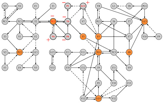
Figure 13. The SDG model of the fault situation.

In Figure 13, the key nodes selected by the EW-VIKOR method are marked, which is filled with orange. In the SDG model, it can be seen that the key nodes T5 and F5 are downstream of the abnormal nodes and immediately adjacent to them. Once they are affected by the deviation and transformed into abnormal states, the damage to the whole system is more serious. Therefore the filtered critical nodes are highlighted in identification results. The severity of different faults on the system is distinguished by whether they can affect the critical nodes.

4. Conclusions

A novel DMA-SDG method is put forward to detect and identify the faults of a hydrogenation prefractionation system. The steady-state simulation of hydrogenation pre-fractionation is established based on the data parameters provided by petrochemical enterprise. The relative errors of pressure, temperature, and flow rate between simulated values and actual values are less than 2%. Fifty-four variables in this system including flow rate, temperature, pressure, liquid level and valve opening are controlled through adding eight controllers and setting accurate operating parameters in dynamic simulation. The SDG model accurately describes the characteristics of the fault through the information propagation path between nodes with alarm thresholds. The theory of complex networks is introduced into SDG and 54 variables are ranked by the EW-VIKOR method. Eight key variables are finally selected and their importance is elaborated from a practical engineering perspective. Comparison of the severity of different alarms is performed by key variables. This method can combine the dynamic simulation results with the SDG model to give a reasonable explanation for the fault. The conclusion observed in this research suggests the potential application of DMA-SDG method to more real production systems, such as catalytic cracking systems and crude oil systems. In the future work, the combination of SDG and complex network can also be applied to fault classification alarm and evaluation.

References

- Sun, W.; Paiva, A.R.C.; Xu, P.; Sundaram, A.; Braatz, R.D. Fault detection and identification using Bayesian recurrent neural networks. Comput. Chem. Eng. 2020, 141, 106991. [Google Scholar] [CrossRef]
- Daher, A.; Hoblos, G.; Khalil, M.; Chetouani, Y. Parzen window distribution as new membership function for ANFIS algorithm-Application to a distillation column faults prediction. IFAC Pap. 2018, 51, 241–248. [Google Scholar] [CrossRef]
- Kim, J.; Shah, A.U.A.; Kang, H.G. Dynamic risk assessment with bayesian network and clustering analysis. Reliab. Eng. Syst. Saf. 2020, 201, 106959. [Google Scholar] [CrossRef]
- Luyben, W.L. Aspen dynamics simulation of a middle-vessel batch distillation process. J. Process. Contr. 2015, 33, 49–59. [Google Scholar] [CrossRef]
- Negrellos-Ortiz, I.; Flores-Tlacuahuac, A.; Gutiérrez-Limón, M.A. Dynamic optimization of a cryogenic air separation unit using a derivative-free optimization approach. Comput. Chem. Eng. 2018, 109, 1–8. [Google Scholar] [CrossRef]
- Cui, Z.; Tian, W.; Fan, C.; Guo, Q. Novel design and dynamic control of coal pyrolysis wastewater treatment process. Sep. Purif. Technol. 2020, 241, 116725. [Google Scholar] [CrossRef]
- Luyben, W.L. Rigorous dynamic models for distillation safety analysis. Comput. Chem. Eng. 2012, 40, 110–116. [Google Scholar] [CrossRef]
- Cui, Z.; Tian, W.; Wang, X.; Fan, C.; Guo, Q.; Xu, H. Safety integrity level analysis of fluid catalytic cracking fractionating system based on dynamic simulation. J. Taiwan Inst. Chem. E 2019, 104, 16–26. [Google Scholar] [CrossRef]
- Zhu, J.; Hao, L.; Bai, W.; Zhang, B.; Pan, B.; Wei, H. Design of plantwide control and safety analysis for diethyl oxalate production via regeneration-coupling circulation by dynamic simulation. Comput. Chem. Eng. 2019, 121, 111–129. [Google Scholar] [CrossRef]
- Carlos, M.; Fatine, B.; Nelly, O.; Nadine, G. Deviation propagation analysis along a cumene process by using dynamic simulations. Comput. Chem. Eng. 2018, 117, 331–350. [Google Scholar] [CrossRef]
- Taqvi, S.A.; Tufa, L.D.; Zabiri, H.; Maulud, A.S.; Uddin, F. Fault detection in distillation column using NARX neural network. Neural Comput. Appl. 2020, 32, 3503–3519. [Google Scholar] [CrossRef]
- Taqvi, S.A.; Tufa, L.D.; Zabiri, H.; Maulud, A.S.; Uddin, F. Multiple fault diagnosis in distillation column using multikernel support vector machine. Ind. Eng. Chem. Res. 2018, 57, 14689–14706. [Google Scholar] [CrossRef]
- Tian, W.; Du, T.; Mu, S. HAZOP analysis-based dynamic simulation and its application in chemical processes. Asia Pac. J. Chem. Eng. 2015, 10, 923–935. [Google Scholar] [CrossRef]
- Rashidi, B.; Singh, D.S.; Zhao, Q. Data-driven root-cause fault diagnosis for multivariate non-linear processes. Control Eng. Pr. 2018, 70, 134–147. [Google Scholar] [CrossRef]
- Djeziri, M.A.; Benmoussa, S.; Mouchaweh, M.S.; Lughofer, E. Fault diagnosis and prognosis based on physical knowledge and reliability data: Application to MOS field-effect transistor. Microelectron. Reliab. 2020, 110, 113682. [Google Scholar] [CrossRef]
- Zhao, H.; Liu, J.; Dong, W.; Sun, X.; Ji, Y. An improved case-based reasoning method and its application on fault diagnosis of Tennessee Eastman process. Neurocomputing 2017, 249, 266–276. [Google Scholar] [CrossRef]
- Tang, K.H.D.; Md Dawal, S.Z.; Olugu, E.U. Integrating fuzzy expert system and scoring system for safety performance evaluation of offshore oil and gas platforms in Malaysia. J. Loss Prev. Proc. 2018, 56, 32–45. [Google Scholar] [CrossRef]
- He, B.; Chen, T.; Yang, X. Root cause analysis in multivariate statistical process monitoring: Integrating reconstruction-based multivariate contribution analysis with fuzzy-signed directed graphs. Comput. Chem. Eng. 2014, 64, 167–177. [Google Scholar] [CrossRef]
- Peng, D.; Gu, X.; Xu, Y.; Zhu, Q. Integrating probabilistic signed digraph and reliability analysis for alarm signal optimization in chemical plant. J. Loss Prev. Proc. 2015, 33, 279–288. [Google Scholar] [CrossRef]
- Reinartz, C.; Kirchhübel, D.; Ravn, O.; Lind, M. Generation of signed directed graphs using functional models. IFAC Pap. 2019, 52, 37–42. [Google Scholar] [CrossRef]
- Smaili, R.; El Harabi, R.; Abdelkrim, M.N. Design of fault monitoring framework for multi-energy systems using signed directed graph. IFAC Pap. 2017, 50, 15734–15739. [Google Scholar] [CrossRef]
- Gao, D.; Wu, C.; Zhang, B.; Ma, X. Signed directed graph and qualitative trend analysis based fault diagnosis in chemical industry. Chin. J. Chem. Eng. 2010, 18, 265–276. [Google Scholar] [CrossRef]
- Yang, Y.; Yu, L.; Wang, X.; Zhou, Z.; Chen, Y.; Kou, T. A novel method to evaluate node importance in complex networks. Phys. A Stat. Mech. Appl. 2019, 526, 121118. [Google Scholar] [CrossRef]
- Iri, M.; Aoki, K.; O’Shima, E.; Matsuyama, H. An algorithm for diagnosis of system failures in the chemical process. Comput. Chem. Eng. 1979, 3, 489–493. [Google Scholar] [CrossRef]
- Luyben, W.L. Distillation Design and Control Using Aspen Simulation, 2nd ed.; Wiley: Hoboken, NJ, USA, 2013; pp. 100–111. [Google Scholar]
- Li, A.; Xia, T.; Zhang, B.; Zhang, Z.; Wu, Z. SDG modeling approach for chemical engineering process. J. Syst. Simul. 2003, 15, 1364–1368. [Google Scholar]
Publisher’s Note: MDPI stays neutral with regard to jurisdictional claims in published maps and institutional affiliations. |
© 2021 by the authors. Licensee MDPI, Basel, Switzerland. This article is an open access article distributed under the terms and conditions of the Creative Commons Attribution (CC BY) license (http://creativecommons.org/licenses/by/4.0/).