Abstract
Quality prediction in the continuous casting process is of great significance to the quality improvement of casting slabs. Due to the uncertainty and nonlinear relationship between the quality of continuous casting slabs (CCSs) and various factors, reliable prediction of CCS quality poses a challenge to the steel industry. However, traditional prediction models based on domain knowledge and expertise are difficult to adapt to the changes in multiple operating conditions and raw materials from various enterprises. To meet the challenge, we propose a framework with a multiscale convolutional and recurrent neural network (MCRNN) for reliable CCS quality prediction. The proposed framework outperforms conventional time series classification methods with better feature representation since the input is transformed at different scales and frequencies, which captures both long-term trends and short-term changes in time series. Moreover, we generate different category distributions based on the random undersampling (RUS) method to mitigate the impact of the skewed data distribution due to the natural imbalance of continuous casting data. The experimental results and comprehensive comparison with the state-of-the-art methods show the superiority of the proposed MCRNN framework, which has not only satisfactory prediction performance but also good potential to improve continuous casting process understanding and CCS quality.
1. Introduction
At present, the steel industry is facing unprecedented challenges including resource consumption, serious environmental pollution, substandard process and product stability, and low productivity [1]. Steelmaking is a typical process industry, with long production processes, complicated manufacturing processes, and many process control factors involved [2]. The changes in product types and raw materials of different companies will be different, and it is difficult for knowledge-based models to adapt to all changes, which makes the migration and maintenance of models difficult. Therefore, the deep integration of information technology and the steel manufacturing industry, as the entry point for industrial upgrading, is of great significance to the realization of intelligent and green steel production.
Continuous casting is the most critical part of steelmaking [3]. Stable and high-quality continuous casting production is the top priority of iron and steel enterprises. Continuous casting is the process of solidifying molten metal into semifinished slabs and rolling them in a finishing mill [4]. As shown in Figure 1, the molten metal is transferred from the ladle to a tundish and slowly injected into the continuous caster. Then, the crystallizer in the continuous caster shapes the casting and rapidly solidifies and crystallizes. In this process, the mold level fluctuation will greatly affect the quality of continuous casting slabs (CCSs). With the sharp fluctuation of the liquid level in the mold, the content of oxide inclusions under the slabs will increase significantly [5]. However, mold level fluctuation is likely to cause slag entrapment of molten steel, which further leads to the deterioration of slab quality.
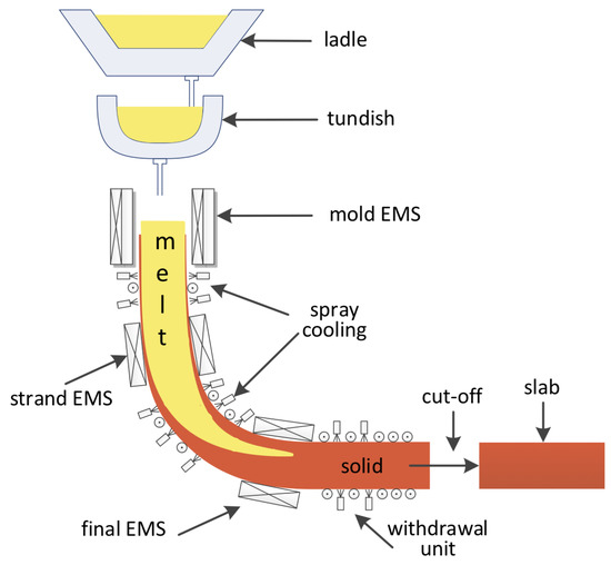
Figure 1.
A schematic diagram of the continuous casting process.
Major steel producers are leveraging information technology such as the Internet of Things (IoT) and embracing big data to change the current state of the steel industry [6]. The use of sensor-based data acquisition systems in factories and the explosive growth of steel data make data modeling and analysis possible [7]. Furthermore, over the last decade, intelligent technologies, represented by data mining [8] and neural networks [9], have been developed from the theoretical research into their industrial applications. In the field of steelmaking, numerous scholars focus on the classification of steel surface defects [10,11]. Although continuous casting is the main process phase affecting the final quality of the steel products, the continuous casting system has a large number of complex input parameters; thus it is well adapted for big data analysis. Lei et al. have used machine learning methods to develop an offline system for continuous casting data collection and data mining [12], a small amount of research work involves the classification and prediction of continuous casting slabs quality. Nandkumar et al. [13] predicted and improved the quality of iron casting with the Six Sigma approach. A two-layer feedforward backpropagation neural network model was developed to predict the possibility of defects in foundry products [14]. The feedforward backpropagation neural net is out of practice currently, and the vanilla recurrent neural net performs poorly in engineering. Artur et al. designed a specific convolutional neural network (CNN) to detect stickers during continuous casting [15]. Although their method can reduce false alarms, when CNN is used alone for detection, the effect is not respectable. Indeed, we have incorporated two neural net architectures into our multiscale convolutional and recurrent neural network (MCRNN) to build one more robust and better network.
In this work, based on the process data acquisition system, a real-time prediction closed-loop control system was constructed to predict and improve the quality of CCS. In the system, a framework composed of an MCRNN is proposed for real-time quality prediction of CCS. Various conversions are made at different times and frequencies to obtain time series data for fluctuations in the level of the original mold. The CNN can apply to time series analysis of sensor data well, and it can also be used to analyze signal data with a fixed-length period. Feature extractors based on the fully convolutional network (FCN) and long short-term memory (LSTM) are used to capture long-term dependencies and extract local features of time series, respectively, and we use the advantages of CNN to automatically learn features [16] in the downsampling transformation representation and frequency domain, extracting features of different time scales and frequencies and solving the limitations of many previous features that can only be extracted at a single time scale [17,18]. As a result, the proposed MCRNN enhances feature representation and improves the performance of quality prediction compared to traditional time series classification models. Moreover, the number of normal samples is much larger than the number of abnormal samples. Average production is 100 slabs, with production of only 5 abnormal slabs. We use the random undersampling (RUS) method to reduce the number of majority classes to address the class imbalance. We introduced expert knowledge into the system. When the predictive model detects an abnormal slab, the continuous casting process adjusts in real-time based on expert knowledge, which improves steelmaking efficiency and slab quality.
The organizational structure is as follows: In Section 2, we review the work related to time series classification. In Section 3, we describe our proposed MCRNN and established system in detail, which is the core section of the paper. In Section 4, we present the detailed process and experimental results of the method. Finally, in Section 5, we draw the main conclusions of this work.
2. Related Work
In our real world, time series data are ubiquitous; examples include temperature, click volume, stock prices, and sensor data. They are sequential data of real value type with a large amount of data, high data dimensions, and constant updating of data. In the data-driven era, there is an increasing demand for information extracted from time series, the main task of which is time series classification (TSC). It is a long-standing problem involving a wide range of practical applications, such as the classification of financial time series [19], the judgment of individual agricultural land-cover types [20], and early churn detection [21].
Traditional time series classification methods are mostly based on distance measurement. Lines and Bagnall [22] proposed nearest neighbor classifiers with elastic distance measures to improve classification accuracy. In particular, the dynamic time warping (DTW) distance combined with the nearest neighbor classifier has proved to be a strong baseline [23]. Nevertheless, the performance could be rarely acceptable when it was applied to the engineering field with big data. There are other methods of distance measurement and spatial transformation for time series, such as information entropy [24], weighted dynamic time warping (WDTW) [25], and shapelet transformation [26]. Moreover, enhanced weighted dynamic time warping [27] and distributed fast-shapelet transform [28] were proposed to improve the performance of times series classification. Based on ensemble schemes and data conversion, Bagnall et al. not only aggregated different classifiers on the same transformation but also collected different classifiers in different time series representations [29]. However, these methods only have linear separability.
In recent years, deep learning has developed rapidly and achieved excellent results in classification tasks. Convolutional neural networks and recurrent neural networks are widely used in image recognition [30], video classification [31], machine translation [32], information extraction [33], and other fields. CNN can use convolutional layers to learn complex feature representations automatically, with the advantage of absorbing a large amount of data to learn feature representations. In recent years, many neural networks for time series classification, such as multilayer perceptron (MLP), fully convolutional network (FCN), and residual network (ResNet) [34], emerged. Convolutional neural networks (CNN) have been applied to time series applications, though CNN is mainly for the image field [35,36]. In the classification of high-dimensional time series, Zheng et al. proposed to use a multichannel convolutional neural network for modeling [37]. The echo state network (ESN) is a time-warping invariant, limited to static patterns rather than temporal patterns, and was applied to time series classification tasks [38]. Joan et al. studied the use of a time series encoder and established a hybrid deep CNN with an attention mechanism [39]. For the quality prediction system, however, these present methods cannot meet the demands of overall continuous casting slab production pipelines.
3. Methodology
Given a series of mold level fluctuations, our goal is to predict the quality of the continuous casting slab (CCS) in production. The quality of CCS will also change under different production conditions, such as different raw materials and technological parameters. In addition, it is worth noting that the quality of CCS is normal in most cases, while only a few are abnormal. Unbalanced time series classification is a challenging task when using only FCN or LSTM to extract time series on a single scale. We consider that time series should be represented comprehensively in multiscale and multifrequency dimensions to improve the classification performance and obtain a robust model. To address these problems for quality prediction of the CCS, we propose a new MCRNN architecture, where the input is the time series of mold level fluctuation to be predicted and the output is its quality label, as shown in Figure 2. The more details of layouts of each network are tabulated in Table 1. We use the grid search to obtain hyperparameters and iteratively find the best hyperparameters. This architecture mainly includes three sequential stages: the input representation stage, the feature learning stage, and the classification stage.
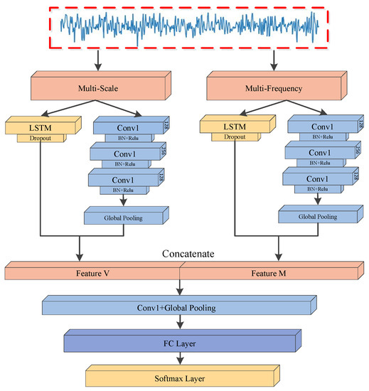
Figure 2.
The proposed multiscale convolutional and recurrent neural network (MCRNN) framework.

Table 1.
Details of the the MCRNN structure.
3.1. Class Imbalance
In the process of quality prediction, the number of abnormal and normal samples is extremely unbalanced, and the imbalance ratio is about 20:1. Class imbalance can have a negative impact on classification performance, because the classifier trained on unbalanced data favor major classes. We utilize the RUS method to achieve a more balanced class distribution, which improves the classification performance.
The RUS method is a form of data sampling that randomly selects major class instances and removes them from the dataset until the desired class distribution is achieved. Based on the original unbalanced dataset, RUS is used to generate the training dataset of three sample ratios, which are 1:1, 1:2, and 1:3. The normal sample ratio is followed by the abnormal sample ratio. We try to see how different sampling ratios affect the classification performance of the trained neural network and select the best sampling dataset. However, the test set is generated from unbalanced raw data without RUS because of realistic prediction requirements. As shown in Figure 3, in the original dataset of continuous casting slabs, the number of abnormal continuous casting slabs is far less than the number of normal continuous casting slabs. The desired class distribution is achieved by randomly removing the normal CCS and retaining the entire abnormal CCS, which can cause the loss of majority class information.
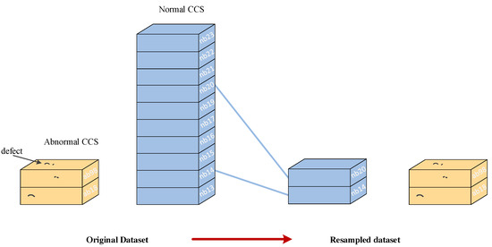
Figure 3.
The random undersampling process of continuous casting slabs (CCSs).
3.2. MCRNN Architecture
3.2.1. Input Representation
Consideration should be given to using multiscale time series to build an accurate and reliable time series model. The long-term temporal pattern shows general trend changes, and the short-term temporal pattern reflects fine-grained fluctuations. Both patterns are critical to the performance of TSC. In our research work, we transform the original input space to obtain representation at different time scales and frequencies inspired by Cui et al. [40]. The transformation includes two stages: downsampling transformation in the time domain and smoothing transformation in the frequency domain. In the first stage, we downsample from the sequence of mold level fluctuation and the downsampling rate is r. Then, new time series is generated from the original sequence by retaining every data points.
Due to the influence of high-frequency disturbances and random noise, we carry out the moving average of the time series in the second stage to solve the problem. Given an original sequence of mold level fluctuation, a new time series can be defined as according to different degrees of smoothness.
where w is the window size.
As shown in Figure 4, a sequence of the mold level fluctuation values in the production time of one slab transforms in time and frequency dimensions. For different downsampling rates and degrees of smoothness, we can get multiple time sequences, each of which corresponds to different scale representations of original sequence input. With the multiscale transformation of input, long-term temporal patterns and short-term temporal patterns can be employed to build a robust model. At the same time, the new time series based on the moving average of different windows reduces the noise of the original sequence. After two stages of transformation, the input is divided into two modules and fed into the neural network. For r and w, it is related to the sampling size. Sampling size is the sample points for each slab. We compared the sampling size values when the sampling rate is 1:2. As shown in Table 2, the model trained well when the sampling size was equal to 256, so we use 256 in our model.
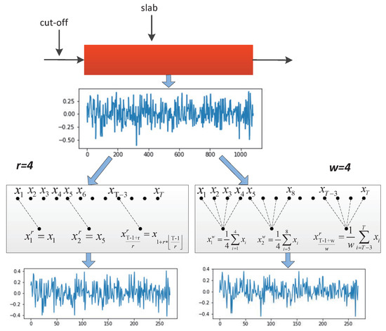
Figure 4.
Illustration of the input transformations when r = 4 and w = 4.
Table 2.
Comparison of sampling size with sampling ratios = 1:2.
3.2.2. Feature Learning
The feature extractor architecture is composed of the LSTM module and a fully convolutional module. The goal of this phase is to learn effective time series features in a parallel manner through multiple pairs of recurrent layers and convolutional layers in advance.
- LSTM module: This module contains an LSTM layer, followed by a dropout layer. We employ an LSTM feature extractor to capture temporal patterns of CCS time series with multiscale and multifrequency dimensions. Specifically, the mold level fluctuation input and the hidden state of the previous time step given for the time step t. The definition of input gate , forget gate , and output gate is as follows. The input gate controls the extent to which a new value flows into the cell.The forget gate decides what information should be dropped.The output gate determines which parts are useful.The candidate memory cells at time step t are calculated asThe calculation of the current time step memory cell combines the information of the last time step memory cell and the current time step candidate memory cell, and controls the flow of information through the forgetting gate and the input gate.The output gate controls the flow of information from memory cells to the hidden state , which can be calculated as:We feed the raw or transformed mold level fluctuation to LSTM and get output vector from the last layer of the LSTM. We use output at time step t as feature extracted by LSTM. To prevent overfitting, the output of the LSTM layer is followed by the dropout layer with a dropout rate of 0.8 as shown in Figure 2. With dropout, final feature vector can denote as:Here, * denotes an element-wise product. For output vector at time step t, is a vector of independent random variables, each of which has probability p of being 1.
- Fully convolutional module: The core component of fully convolutional module is a convolutional block that contains:
- Convolutional layer with a filter size of 128 or 256, the kernel with a size of 8, 5, 3 and stride of 1.
- Batch normalization layer with a momentum of 0.99 and epsilon of 0.001.
- A ReLU activation at the end of the module.
In this module, we utilize convolution kernel to slide over the input sequence and extract local features. The output of the i-node in the feature map is defined bywhere represents m-length subsequence from the ith time step to the th time step of input sequence, * denotes the convolution operator, b denotes the bias term, and is a nonlinear activation function.Accordingly, the convolution kernel is slid from the beginning time step to the end and we get the feature map of the jth kernel as
After convolution, batch normalization followed by a ReLU activation function accelerates fast training speed and improves model generalization ability. The fully convolutional module contains three convolutional blocks which are used as a feature extractor. Then, it performs a one-dimensional global average pooling operation on the feature map of the last block to obtain the vector, which reduces feature dimensions while increasing the receptive field of the kernel. The vector obtained by global average pooling on the final output channel can be expressed as
where k represents the filter size of the last convolutional block. We concatenate the features extracted by LSTM with a fully convolutional module. As mentioned in the previous section, the original input is transformed at different time scales and frequencies, so we use feature extractors on different input expressions and feed the final features into the next stage as input.
3.2.3. Classification
Finally, the concatenated feature vector obtained in the feature learning stage is directly fed to the classification module, which is composed of a convolution and global average pooling layer, a fully connected layer, and a softmax layer. As a result, it outputs conditional probability for each class. The softmax function rescales the n-dimensional vector of the FC layer output so that the output value is in the range [0, 1] and the sum is 1, which is defined by the following:
The full convolution module and LSTM module process the same time series input in two different fields of view. The full convolution is a fixed-size perception field to extract local features of time series. On the contrary, LSTM effectively captures time dependencies. The method of combining with convolutional and recurrent neural networks is crucial to enhance the performance of the proposed framework.
3.3. Quality Prediction System Based on MCRNN
Based on a large amount of process information collected by sensors, a quality prediction and control system is established for intelligent decision-making and control. To elaborate on the infrastructure of an established system, the framework of the system based on MCRNN is described in Figure 5. It mainly consists of three parts: data acquisition, quality prediction, and dynamic control. Data acquisition module based on various sensor networks collects massive real-time production data about the continuous casting process, such as temperature, water volume, and casting speed. The real-time collected process data will be sent to the quality prediction module and stored as historical data for visualizing the display and training of the model. Moreover, the quality information of each rolled slab is collected to label continuous casting data.
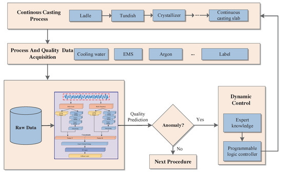
Figure 5.
The framework of quality prediction system based on MCRNN.
With production process parameters and slab labels, a quality prediction model based on the proposed MCRNN is built. In the real-time production process, the original time series data are entered into the model and transformed with different time scales and frequencies. The output of the model is the quality label of CCS. Once the slab in producing is judged to be abnormal by the prediction model, the knowledge of domain experts will be employed to dynamically adjust the production process. The dynamic control module adjusts the process and equipment parameters in time through the programmable logic controller to avoid affecting the next rolling process and causing waste. Abnormal CCS produced will be sorted into the cleaning process of the machine to eliminate defects. The workflow improves efficiency, reduces costs, and enhances yield greatly.
4. Experiments and Results
In this section, we first describe the dataset and the evaluation metrics. Then, the effects of the RUS method and multiscale transformations are discussed in our studies. Finally, the proposed MCRNN model compares with different baseline models.
4.1. Dataset
Based on the installed data collector, the mold level fluctuation of the continuous casting production is recorded every 0.5 s in time series. In this way, we obtain a one-year continuous casting real-time process (CCRP) dataset which is not labeled. The continuous casting slab is rolled, and then the label information is generated by the inspection machine. Therefore, we get slightly delayed slab quality information, called the slab label dataset, from another system.
The slab label dataset contains abnormal reasons to be used as anomaly labels. We cannot obtain the quality information of CCS in the production process immediately, and can only get feedback results after hot rolling. The only connection to the CCRP dataset and the slab label dataset is the time of continuous casting. We map the anomaly labels in the slab label dataset to the CCRP dataset through casting time. Each slab corresponds to a large amount of real-time information during the continuous casting period. With the help of the start and end times in the slab label dataset, we match quality labels to the time series data during this period.
After marking the CCRP dataset with the slab label dataset, we obtained 9628 time series of slabs with the label. Among them, 9073 time-series were labeled as normal samples, and 555 time series were labeled as abnormal samples. In all experiments, we used a leave-one-out approach to train and test the classifier, divided the sample into two, 70% of the samples for training and 30% of the samples for testing, and used k-fold cross-validation to ensure the robustness of the model; cross-validation was repeated 5 times. However, normal and abnormal samples were extremely unbalanced. We utilized the RUS method described in Section 3.3 on the training set to ensure sample balance.
4.2. Evaluation Metrics
The confusion matrix is used to evaluate the quality of the algorithm in the classification task. In particular, we focus on three important metrics, the average accuracy of the classifier, the recall value for each class, and score. Our goal is to find a balance between false negatives and false positives, and find as many abnormal slabs as possible for good judgment. Specifically, if our model does not detect a CCS with abnormal quality, the abnormal slab will move on to the next process, and the final result is that the produced steel plate cannot be sold. If a CCS of normal quality is predicted to be abnormal by the model, it will undergo further processing attempts to change the quality status, which will increase costs. The most important point is that the cost of sending defective products to customers can be much higher than that of inspecting the products. Therefore, we want to maximize recall rates of exception class and sacrifice as few normal samples as possible.
where i refers to class index and represents the proportion of samples of class i, with being the number of samples of the ith class and N being the total number of samples.
4.3. Effect of Random Undersampling
The training errors of different sampling rates (1:1, 1:2, 1:3) shows in the form of loss curves in Figure 6. When the sampling rate is 1:2, the curve drops more smoothly, so the sampling effect is better.
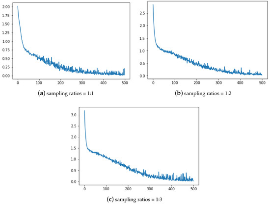
Figure 6.
The MCRNN training loss curve with different sampling ratios.
Table 3, Table 4 and Table 5 show the results of k-fold cross-validation of the proposed MCRNN method at different sampling rates, k = 5. The result of the proposed MCRNN method at different sampling ratios is shown in Table 6. From the results, we can see the effect of sampling on the predictive performance of the model, and our model has a certain degree of robustness. Without sampling, recall for abnormal class and normal class is 0 and 1, respectively. Obviously, the trained models predicted all the slabs as normal to acquire the highest accuracy, without any ability to detect abnormal slabs. As the proportion of abnormal samples in the training sample increases, the recall of abnormal class increases. The SMOTE sampling algorithm has a certain effect on solving the problem of imbalanced data [41]. We also compared the SMOTE sampling algorithm with RUS in Table 6, and it was obvious that the RUS algorithm we proposed has a better effect on our data set. However, when the sampling ratio is 1:1, although more than 50% of abnormal slabs can be identified, a large number of normal slabs are misjudged at the same time. It is reflected in the low score and accuracy.
Table 3.
Results for sampling ratios = 1:1 with k = 5.
Table 4.
Results for sampling ratios = 1:2 with k = 5.
Table 5.
Results for sampling ratios = 1:3 with k = 5.
Table 6.
Results for different sampling ratios.
Through the sampling of training samples, the prediction ability of the model for abnormal slab can be improved, but the best proportion is one that is not completely balanced. When the sampling ratio is 1:2 or 1:3, the trained model has a certain ability to detect abnormal slabs without misjudging a large number of normal slabs. In the actual quality prediction of CCS, we adopt the sampling strategy with a sampling ratio of 1:2 because sending defective slabs to customers based on prediction can be more expensive than misjudgment, and we want to detect as many abnormal slabs as possible to avoid inferior products.
4.4. Effect of Multiscale Transformations
In order to validate the effectiveness of multiscale input transformations, we performed experiments with transformed and untransformed inputs. The results are shown in Figure 7. We can see that the score with input transformations is higher than that without input transformations when the sampling ratio is 1:2 and 1:3. When the sampling ratio is 1:1, the score of the two scenarios are almost identical. However, input transformations have a positive effect on the recall for abnormal class. It can be concluded from the right part of the figure that more abnormal slabs can be detected with input transformations. In most cases, performing input transformations will help greatly improve classification performance. The effectiveness of the multiscale transformations is demonstrated in the recall rate of the abnormal class and score.
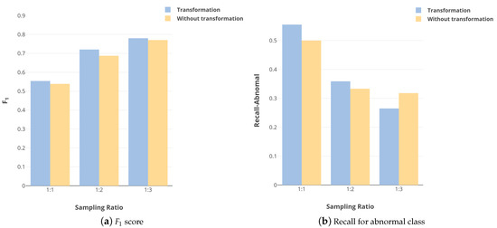
Figure 7.
Effects of multiscale transformation on classification performance.
4.5. Comparison
We conducted experiments on our dataset using two baseline methods from the publication of Wang et al. [34] for comparison to our developed approach: fully convolutional network (FCN) and residual network (ResNet), which have been proved to be useful as standard benchmarks for end-to-end time series classification networks. The FCN basic block is a convolutional layer, followed by a batch of normalization layer and a ReLU activation layer, and the final output comes from the softmax layer. The convolution operation is completed by three 1-D kernels of size 8, 5, 3. The final network is constructed by stacking three convolution blocks. The filter size of each convolution block is 128, 256, 128. ResNet uses the convolution block in FCN to construct each residual block, and finally stacks three residual blocks, followed by a global average pooling layer and a softmax layer. The number of filters for each residual block is 64, 128, 128. Furthermore, long short-term memory (LSTM) is used to compare with our proposed method, which has been proved to apply to periodic time series data. We have optimized the parameters of all networks participating in the comparison experiment to achieve the best results in this problem domain.
Table 4 shows the recall rate for the abnormal class of the proposed model and the other methods of baselines. Table 5 compares the score of our proposed model with other models. The results illustrate that our proposed model achieves the highest recall for abnormal class at different sampling ratios. According to Table 7 and Table 8, the proposed model achieves the highest recall for abnormal class while maintaining a high score. When the sampling ratio is 1:2, the proposed model obtains the recall for an abnormal class of 0.3590 and the of 0.7207. It is best for our task. We hope that the model can detect more abnormal slabs and minimize misjudgment, which is a cost consideration.
Table 7.
Recall-Abnormal comparison between the proposed model and the other baseline methods.
Table 8.
score comparison between the proposed model and the other baseline methods.
By comparison of the three methods, LSTM is bad in comparison to ResNet and FCN for Recall-Abnormal and MCRNN is not superior to ResNet and FCN in the score. However, the MCRNN is superior to LSTM in the Recall-Abnormal score, though the MCRNN shows inferior slightly to LSTM in the score. Considering the engineering scenario of steel production prediction, the Recall-Abnormal is more important than the score to prevent low-level steel slabs from escaping check. FCN and ResNet, though slightly inferior to our model, also achieved good classification performance. However, LSTM performs unsatisfactorily in most cases except for the 1:1 sampling ratio. LSTM can easily deal with periodic time series data, but there are still some challenges with cluttered sensor data. Compared with FCN and ResNet, the MCRNN extracts features at different time scales and frequencies. Inputs of different transformations capture long-term trends and short-term changes, which is essential for classification. It can explain that the traditional methods simply perform a large number of convolutions over the same time scale.
5. Conclusions
We proposed a novel MCRNN architecture for the quality prediction of CCS. The major contributions of the new architecture are the transformations of time series input and feature extraction with LSTM and FCN. The proposed architecture can automatically extract the long-term trend and short-term change of time series, which greatly enhances feature learning ability and abnormal slab detecting performance. Extensive experimental results show that traditional methods are more incapable when dealing with messy and unbalanced data, and multiscale convolution and recurrent neural networks outperform other state-of-the-art baseline methods in quality prediction. Accordingly, a real-time quality prediction system based on MCRNN architecture has also been developed. The mold level fluctuation collected by the data module in the system is fed into the trained model. The continuous casting process will be adjusted in real-time based on expert knowledge if there is a high probability of prediction that it is an abnormal slab. The system greatly enhances steelmaking efficiency, improves slab quality, and reduces costs. Due to class imbalance caused by a few abnormal slabs, we use a random sampling method to generate training sets with three different sampling ratios to help mitigate class imbalance. Experimental results demonstrated that the proposed method can detect more abnormal slabs and reduce the misjudgment of normal slabs when the sampling ratio is 1:2.
For future research, although the established quality system has achieved certain results, it is still insufficient in several aspects such as interpretability of prediction and root cause analysis, the sampling method of dealing with the problem of unbalanced data is still worthy of our continued study. In recent years, the interpretability of deep learning is an important research field. In the future, we will utilize the interpretable method and root cause analysis to find out the cause of the abnormal slab, which will further improve the performance of intelligent steelmaking.
Author Contributions
X.W., H.J., X.Y. and J.W. (Jianjia Wang) are the main authors of this manuscript. All the authors contributed to this manuscript. Conceptualization, X.W.; data curation, J.W. (Jianjia Wang); methodology, X.W.; software, H.J. and X.Y.; validation, X.Y. and J.W. (Jianjia Wang); writing—original draft preparation, H.J. and X.Y.; writing—review and editing, X.W., H.J., X.Y., J.W. (Jianjia Wang), Z.L., Y.L., J.W. (Jie Wang) and Y.G.; supervision, X.W. All authors have read and agreed to the published version of the manuscript.
Funding
This work was supported by the Natural Science Foundation of Shanghai, China (Grant No. 20ZR1420400), the State Key Program of National Natural Sc hasience Foundation of China (Grant No. 61936001).
Institutional Review Board Statement
Not applicable.
Informed Consent Statement
Not applicable.
Data Availability Statement
Data is contained within the article.
Acknowledgments
We appreciate the High Performance Computing Center of Shanghai University, and Shanghai Engineering Research Center of Intelligent Computing System (No. 19DZ2252600) for providing the computing resources.
Conflicts of Interest
The authors declare no conflict of interest.
Abbreviations
The following abbreviations are used in this manuscript:
| CCS | Continuous Casting Slabs |
| MCRNN | Multiscale Convolutional and Recurrent Neural Network |
| RUS | Random Undersampling |
| IoT | Internet of Things |
| CNN | Convolutional Neural Network |
| LSTM | Long Short-Term Memory |
| TSC | Time Series Classification |
| DTW | Dynamic Time Warping |
| WDTW | Weighted Dynamic Time Warping |
| FCN | Fully Convolutional Network |
| MLP | Multilayer Perceptron |
| ESNs | Echo State Networks |
| CCRP | Continuous Casting Real-time Process |
| ResNet | Residual Network |
| SMOTE | Synthetic Minority Oversampling Technique |
References
- Nikiforova, V.A. World steel industry: Current challenges and development trends (analytical overview). Econ. Ind. 2018, 1, 86–114. [Google Scholar] [CrossRef]
- Xiang, F.; Zhi, Z.; Jiang, G. Digital Twins technolgy and its data fusion in iron and steel product life cycle. In Proceedings of the 2018 IEEE 15th International Conference on Networking, Sensing and Control (ICNSC), Zhuhai, China, 27–29 March 2018; pp. 1–5. [Google Scholar]
- Mazumdar, D. Review, Analysis, and Modeling of Continuous Casting Tundish Systems. Steel Res. Int. 2019, 90, 1800279. [Google Scholar] [CrossRef]
- Louhenkilpi, S. Continuous casting of steel. In Treatise on Process Metallurgy; Elsevier: Boston, MA, USA, 2014; pp. 373–434. [Google Scholar]
- Smirnov, A.; Kuberskii, S.; Smirnov, E.; Verzilov, A.; Maksaev, E. Influence of meniscus fluctuations in the mold on crust formation in slab casting. Steel Transl. 2017, 47, 478–482. [Google Scholar] [CrossRef]
- Peters, H. How could industry 4.0 transform the steel industry? In Proceedings of the Future Steel Forum, Warsaw, Poland, 14–15 June 2017. [Google Scholar]
- Kuo, Y.H.; Kusiak, A. From data to big data in production research: The past and future trends. Int. J. Prod. Res. 2019, 57, 4828–4853. [Google Scholar] [CrossRef]
- Ge, Z.; Song, Z.; Ding, S.X.; Huang, B. Data mining and analytics in the process industry: The role of machine learning. IEEE Access 2017, 5, 20590–20616. [Google Scholar] [CrossRef]
- Xing, S.; Ju, J.; Xing, J. Research on hot-rolling steel products quality control based on BP neural network inverse model. Neural Comput. Appl. 2019, 31, 1577–1584. [Google Scholar] [CrossRef]
- Liu, Y.; Geng, J.; Su, Z.; Zhang, W.; Li, J. Real-time classification of steel strip surface defects based on deep CNNs. In Proceedings of 2018 Chinese Intelligent Systems Conference; Springer: Singapore, 2019; pp. 257–266. [Google Scholar]
- He, D.; Xu, K.; Wang, D. Design of multi-scale receptive field convolutional neural network for surface inspection of hot rolled steels. Image Vis. Comput. 2019, 89, 12–20. [Google Scholar] [CrossRef]
- Lei, Z.; Li, B.; Zhou, Y.; Wu, X.; Zhong, Y.; Ren, Z. Two Paradigms on Study Slab Continuous Casting Process with Mold Electromagnetic Stirring. MS&E 2018, 424, 012035. [Google Scholar]
- Mishra, N.; Rane, S.B. Prediction and improvement of iron casting quality through analytics and Six Sigma approach. Int. J. Lean Six Sigma 2019, 10, 189–210. [Google Scholar] [CrossRef]
- Hore, S.; Das, S.K.; Humane, M.M.; Peethala, A.K. Neural Network Modelling to Characterize Steel Continuous Casting Process Parameters and Prediction of Casting Defects. Trans. Indian Inst. Met. 2019, 72, 3015–3025. [Google Scholar] [CrossRef]
- Faizullin, A.; Zymbler, M.; Lieftucht, D.; Fanghänel, F. Use of Deep Learning for Sticker Detection During Continuous Casting. In Proceedings of the 2018 Global Smart Industry Conference (GloSIC), Chelyabinsk, Russia, 13–15 November 2018; pp. 1–6. [Google Scholar]
- Domingos, P. A few useful things to know about machine learning. Commun. ACM 2012, 55, 78–87. [Google Scholar] [CrossRef]
- Murad, A.; Pyun, J.Y. Deep recurrent neural networks for human activity recognition. Sensors 2017, 17, 2556. [Google Scholar] [CrossRef] [PubMed]
- Minar, M.R.; Naher, J. Recent advances in deep learning: An overview. arXiv 2018, arXiv:1807.08169. [Google Scholar]
- Chao, L.; Zhipeng, J.; Yuanjie, Z. A novel reconstructed training-set SVM with roulette cooperative coevolution for financial time series classification. Expert Syst. Appl. 2019, 123, 283–298. [Google Scholar] [CrossRef]
- Whelen, T.; Siqueira, P. Time-series classification of Sentinel-1 agricultural data over North Dakota. Remote Sens. Lett. 2018, 9, 411–420. [Google Scholar] [CrossRef]
- Óskarsdóttir, M.; Van Calster, T.; Baesens, B.; Lemahieu, W.; Vanthienen, J. Time series for early churn detection: Using similarity based classification for dynamic networks. Expert Syst. Appl. 2018, 106, 55–65. [Google Scholar] [CrossRef]
- Lines, J.; Bagnall, A. Time series classification with ensembles of elastic distance measures. Data Min. Knowl. Discov. 2015, 29, 565–592. [Google Scholar] [CrossRef]
- Bagnall, A.; Lines, J.; Bostrom, A.; Large, J.; Keogh, E. The great time series classification bake off: A review and experimental evaluation of recent algorithmic advances. Data Min. Knowl. Discov. 2017, 31, 606–660. [Google Scholar] [CrossRef]
- Deng, H.; Runger, G.; Tuv, E.; Vladimir, M. A time series forest for classification and feature extraction. Inf. Sci. 2013, 239, 142–153. [Google Scholar] [CrossRef]
- Jeong, Y.S.; Jeong, M.K.; Omitaomu, O.A. Weighted dynamic time warping for time series classification. Pattern Recognit. 2011, 44, 2231–2240. [Google Scholar] [CrossRef]
- Hills, J.; Lines, J.; Baranauskas, E.; Mapp, J.; Bagnall, A. Classification of time series by shapelet transformation. Data Min. Knowl. Discov. 2014, 28, 851–881. [Google Scholar] [CrossRef]
- Anantasech, P.; Ratanamahatana, C.A. Enhanced Weighted Dynamic Time Warping for Time Series Classification. In Third International Congress on Information and Communication Technology; Springer: Singapore, 2019; pp. 655–664. [Google Scholar]
- Baldán, F.J.; Benítez, J.M. Distributed FastShapelet Transform: A Big Data time series classification algorithm. Inf. Sci. 2019, 496, 451–463. [Google Scholar] [CrossRef]
- Bagnall, A.; Lines, J.; Hills, J.; Bostrom, A. Time-series classification with COTE: The collective of transformation-based ensembles. IEEE Trans. Knowl. Data Eng. 2015, 27, 2522–2535. [Google Scholar] [CrossRef]
- Pang, L.; Lan, Y.; Guo, J.; Xu, J.; Wan, S.; Cheng, X. Text matching as image recognition. In Proceedings of the Thirtieth AAAI Conference on Artificial Intelligence, Phoenix, AZ, USA, 12–17 February 2016. [Google Scholar]
- Karpathy, A.; Toderici, G.; Shetty, S.; Leung, T.; Sukthankar, R.; Fei-Fei, L. Large-scale video classification with convolutional neural networks. In Proceedings of the IEEE Conference on Computer Vision and Pattern Recognition, Columbus, OH, USA, 23–28 June 2014; pp. 1725–1732. [Google Scholar]
- Gehring, J.; Auli, M.; Grangier, D.; Yarats, D.; Dauphin, Y.N. Convolutional sequence to sequence learning. In Proceedings of the 34th International Conference on Machine Learning, Sydney, Australia, 6–11 August 2017; Volume 70, pp. 1243–1252. [Google Scholar]
- Stanovsky, G.; Michael, J.; Zettlemoyer, L.; Dagan, I. Supervised open information extraction. In Proceedings of the 2018 Conference of the North American Chapter of the Association for Computational Linguistics: Human Language Technologies, New Orleans, Louisiana; Association for Computational Linguistics (ACL): Stroudsburg, PA, USA, 2018; Volume 1, pp. 885–895, long papers. [Google Scholar]
- Wang, Z.; Yan, W.; Oates, T. Time series classification from scratch with deep neural networks: A strong baseline. In Proceedings of the 2017 International Joint Conference on nEural Networks (IJCNN), Anchorage, AK, USA, 14–19 May 2017; pp. 1578–1585. [Google Scholar]
- Le Guennec, A.; Malinowski, S.; Tavenard, R. Data Augmentation for Time Series Classification Using Convolutional Neural Networks. In ECML/PKDD Workshop on Advanced Analytics and Learning on Temporal Data; halshs: Riva Del Garda, Italy, 2016. [Google Scholar]
- Zhao, B.; Lu, H.; Chen, S.; Liu, J.; Wu, D. Convolutional neural networks for time series classification. J. Syst. Eng. Electron. 2017, 28, 162–169. [Google Scholar] [CrossRef]
- Zheng, Y.; Liu, Q.; Chen, E.; Ge, Y.; Zhao, J.L. Exploiting multi-channels deep convolutional neural networks for multivariate time series classification. Front. Comput. Sci. 2016, 10, 96–112. [Google Scholar] [CrossRef]
- Tanisaro, P.; Heidemann, G. Time series classification using time warping invariant echo state networks. In Proceedings of the 2016 15th IEEE International Conference on Machine Learning and Applications (ICMLA), Anaheim, CA, USA, 18–20 December 2016; pp. 831–836. [Google Scholar]
- Serrà, J.; Pascual, S.; Karatzoglou, A. Towards a Universal Neural Network Encoder for Time Series. arXiv 2018, arXiv:1805.03908. [Google Scholar]
- Cui, Z.; Chen, W.; Chen, Y. Multi-scale convolutional neural networks for time series classification. arXiv 2016, arXiv:1603.06995. [Google Scholar]
- Chawla, N.V.; Bowyer, K.W.; Hall, L.O.; Kegelmeyer, W.P. SMOTE: Synthetic minority over-sampling technique. J. Artif. Intell. Res. 2002, 16, 321–357. [Google Scholar] [CrossRef]


Publisher’s Note: MDPI stays neutral with regard to jurisdictional claims in published maps and institutional affiliations. |
© 2020 by the authors. Licensee MDPI, Basel, Switzerland. This article is an open access article distributed under the terms and conditions of the Creative Commons Attribution (CC BY) license (http://creativecommons.org/licenses/by/4.0/).