Abstract
The recycling rates, especially those from plastic packaging waste, have to be increased according to the European Union directive in the next years. Besides many other technologies, the pyrolysis of plastic wastes seems to be an efficient supplementary opportunity to treat mixed and unpurified plastic streams. For this reason, a pyrolysis process was developed for the chemical recycling of hydrocarbons from waste polyolefins. The obtained products can be further processed and upgraded in crude oil refineries, so that also monomers can be recovered, which are used for the plastic polymerization again. However, to achieve a scale up to a demo plant, a kinetic model for predicting the yields of the plastic pyrolysis in a tubular reactor is needed. For this reason, a pilot plant was built, in which different plastics and carrier fluids can be tested. Based on the data generated at the pilot plant, a very practical and suitable model was found to describe the plastic co-pyrolysis of the carrier fluid with polypropylene (PP) and low density and high density polyethylene (HDPE and LDPE), respectively. The physical and chemical mechanisms of the co-pyrolysis in the tubular reactor are successfully investigated.
1. Introduction
25.8 Mio. tons of plastic waste are produced in Europe annually [1] and less than 30% of this are collected for recycling. Therefore, high amounts of plastic wastes are sent to incineration, landfilling or are sent to non-EU regions [2].
To overcome this situation, the European Union compiled a mandatory goal to reach a recycling rate of plastic packaging waste of 55% in 2030 [3]. The strategy in accomplishing this goal is to enhance a circular economy. The ways of increasing recycling rates include introducing deposit return systems, mechanical recycling, and also chemical recycling via depolymerization and anew polymerization.
However, a common challenge of plastic waste is the sorting of different types of plastics and the contamination of waste streams. Therefore, beside other technologies, pyrolysis is an attractive way to treat mixed plastic or even contaminated streams. In pyrolytic processes, valuable resources are generated out of organic matter at elevated temperatures in absence of oxygen, which can be used as feedstock for refineries and petrochemical industries again [4].
Pyrolysis is a cracking process by breaking long-chain hydrocarbons in molecules with lower molecular weight. These products are liquid and gaseous, respectively, and can be further processed in existing infrastructure, like a conventional crude oil refinery. Thermal cracking (pyrolysis) and catalytic cracking are compared in literature, for example the works [5,6,7,8,9] describe the advantages, disadvantages, technologies and properties of various feedstocks, products and processes. A significant advantage of pyrolysis is the resistance against impurities and the ability to process mixtures of plastic types. All kinds of polyolefins are suitable for pyrolysis because they consist of carbon and hydrogen only without heteroatoms, which then produces valuable yields. Polyolefins, such as polypropylene (PP), low density and high density polyethylene (LDPE and HDPE), are the most used plastics in packaging. Polystyrene (PS) has no heteroatoms and can, thus, be used as feedstock as well. The main challenge in pyrolytic processes is the poor thermal conductivity of plastic. In most waste streams the plastics occur as thin foils or in very voluminous shapes, what makes the handling additionally more complicated. These properties make the necessary heat transfer for thermal cracking difficult. Furthermore, when the plastic is molten, the viscosity is high, and the melt often cannot be pumped with conventional pumps used in refineries.
For operating a commercial plant, high processing capacities and a stable, continuous process is needed to guarantee the feedstock for a refinery. For this reason, a continuous co-pyrolysis process in a tubular reactor was developed [10]. The idea is to use a refinery residue as carrier to fluidize the plastic, consequently it can be treated as a liquid. However, the carrier fluid, also a hydrocarbon, has its own crackability, so the carrier fluid also has to be investigated. Valuable products, which are gaseous at process conditions, as well as solid impurities are separated at the end. The cracking conditions in the tubular reactor are at moderate temperatures below 500 °C and elevated pressures below 25 barg. The process is already verified in lab and pilot scale. A demonstration plant will follow in 2022+. Hence, a simulation and optimization tool must be provided for the upscale. To do so, lumped kinetic modeling was chosen to simplify the complex reaction mechanism [11]. The reactions that take place in the thermal degradation of plastics are radical chain reactions, which results in molecules with lower molecular weight and less saturation. A large amount of species and reactions are involved. These degradation of plastics is often described by thermogravimetric data, and hence, models are received, in which the time depending loss of mass can be measured [8,12,13,14,15,16,17]. Consequently, this kind of models just describe the overall degradation kinetics of polymers. Other models go deeper into the fundamental reactions, such as chain fission, radical recombination, end-chain β-scission and hydrogen transfers, just to mention a few. For this kind of modelling, a high experimental and analytic effort as well as high computational capacity is needed [13,14,18,19].
For upscaling and process optimization, a kinetic model which considers the main parameters, temperature, pressure and residence time, is needed. Furthermore, the model should be simple and should be capable of being integrated in a process simulation tool. Therefore, lumped modeling is used to describe the emerging and vanishing species in a thermal cracking of post-consumer plastics. This approach simplifies the reactions scheme drastically, by grouping (=lumping) species with similar properties together. In this study, a four lump kinetic model, based on boiling points of the species, will be introduced whereby the four lumps are connected with six monomolecular, irreversible, first order reactions. Even with just four reacting pseudo components, the product yields of plastic pyrolysis and the degradation of the carrier fluid can be predicted. However, a model needs reasonable data for verification, so a pilot plant was built in previous works, which can be varied in the main process conditions and feeds [20].
2. Materials and Methods
To observe the effects of temperature, pressure, residence time and plastic type on the product yield of the developed process, a pilot plant was build [20], which is also used for a kinetic study. The formed vaporous products with lower molecular weight are discharged of an unpressurized system as soon as the reaction condition exceed the boiling point. If the cracking process is performed continuously in a tubular reactor, as it is the case in the described process here, the produced gaseous species cannot leave the system, thus parameters like flow rate and pressure have a significant impact on the product yields. Since the pilot plant is diminutive (inner diameter of pipes in the tube reactor is 4.3 mm), the risk of blockages is high. Consequently, the pilot plant is used to investigate pure, virgin plastics and not real, waste plastics. Furthermore, the occurrent plastics in various waste streams are highly diverse, thus it will not be possible to examine all types and all potential mixture configurations of plastic. Hence, reference plastics from all main types are used to get an overview, how the different types of plastic behave in the process. The main feedstock for the thermal degradation process is all kind of polypropylene (PP), low density and high density polyethylene (LDPE and HDPE). Common parameters of the examined plastics types are shown in the next table (Table 1).

Table 1.
Examined plastic types with some measured, descriptive parameters (own measurements).
However, the plastic is pretreated for the usage in the plant. Since no extruder is available for feeding the plastic melt into the pilot plant, a fine plastic powder (<500 µm), obtained by cryogenic grinding, is mixed with the carrier fluid in a certain mixing ratio in a stirring tank.
A test campaign combines different test runs with the specific, investigated plastic type commingled with the carrier fluid. The carrier fluid is a high boiling hydrocarbon and is available on site in the refinery. Therefore, an evaluation of the behavior of the pure carrier fluid has to be done in advance. Tests with pure carrier fluid are run at diverse temperature and residence time couples to measure the conversion rates of the carrier fluid itself under different process conditions. Subsequently, the test series with increasing content of plastic mixed with the carrier fluid are performed again at different process conditions. In this way, the share of the carrier fluid on the observed conversion can be identified. The highest ratio of plastic in the mixture reachable is 30 wt.%, at this plastics content pumping becomes impossible due to the mixture’s increasing viscosity.
2.1. Experimental Setup
The scheme of the pilot plant used for the collection of the process data is shown in Figure 1.
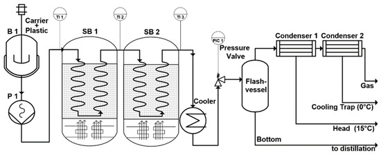
Figure 1.
Scheme of the pilot plant.
In a stirring tank, B1, the plastic powder is mixed with the carrier medium in the specified mixing ratio. Then the mixture is pressed into the reactors by the eccentric screw pump P1. The reactor tubes are immersed in the sand baths SB1 and SB2. Downstream the reactor section, the medium is cooled down in order to instantaneously stop the reaction. The following pressure valve regulates the pressure in the plant. After flashing the products to atmospheric pressure, vaporized products are stripped out and condensed. All products are collected, weighted and analyzed. Density, heating value, paraffinic, aromatic, naphthenic and olefinic content, true boiling point curve are analyzed and a laboratory distillation is performed to calculate the product fraction yields.
The pressure valve can be adjusted from 0–20 barg to adjust the testing condition. This valve is also the bottleneck of the plant because it has the smallest cross section. Therefore, the operating parameters have to be adjusted for achieving a certain range of conversion. A conversion that is too high causes coking and a conversion that is too low results in unconverted plastic or very high molecular waxes. Blocking of the valve occurs in both cases. These limiting factors in the experimental investigations have a big impact on the model, which will be discussed later in the chapter “Lumped model”.
Two sand baths are used for adjustment of the testing temperature. These sand baths have a very homogenous temperature distribution which is achieved by fluidization with air. The coiled reactors are immersed in this sand, whereas reactor tubes wall temperatures are approximately the same as the sand itself. The sand can be heated up to 600 °C to test a wide range of process parameters and resulting achieved conversion rates.
Finally, the residence time can be varied by two different modulations. One is the simple adjustment of the working load of the pump, the second method is to alter the reactor length. Each sand bath can be mounted with reactor coils ranging from 3 to 25 m length, which results in a maximum reactor length of 50 m, if two sand baths are used. The mass flow of the pilot plant can be regulated between 300 and 3000 g/h. Consequently, the maximal production rate of the plant is nearly 1 kg plastic per hour.
2.2. Modelling
The finding and conclusions of the test results of the pilot plant should be used for upscaling a demo plant. To do so, the obtained data should be implemented in a model which can describe engineering relevant phenomena, such as vaporizing, and predict the yield of products. As with other pyrolysis processes, the main influencing parameters of the conversion are temperature, pressure and residence time. The temperature has the major effect, which can be easily explained with the commonly used temperature dependency of reaction rates via the Arrhenius equation. A very minor effect has the pressure on the reaction, often described by Le Chatelier’s principle. Due to the formation of gaseous products, a low pressure is beneficial during pyrolysis. However, since this process takes place in a tubular reactor, the pressure has a greater impact on the residence time due to reduced vaporization at elevated pressures [21]. Finally, the residence time is strongly affected by temperature and pressure. The high vaporization at high temperatures and low-pressure results in high gas phase amounts in the reactor pipes. Consequently, the residence time is reduced, but also the flow regime can change. Hence, the gas to liquid ratio in the system is also an additional physical parameter affecting the reaction by changing the residence time [22].
Since the residence time is the most uncertain parameter, the model is built on a calculation based on the reactor length instead of time. Additionally, the properties of the occurrent media have to be considered to calculate the gas phase share and the resulting volume stream. The analytics of the products and educts are used here to generate pseudo-components, which reflect the educts and products very well. For refinery simulation tools like PetroSim the density and true boiling point curve of a fluid is sufficient to describe this stream and to evaluate its physical properties.
As the temperature, pressure, reactor length and the properties of the mediums are known, the chemical reaction itself has to be described. Since the pilot plant has no continuous measurement, and the plastic pyrolysis produces a multitude of different species because of its radical complexion [22], and additionally, the plant runs at non-idealistic conditions (isothermal reactors cannot be assumed), it is obvious that fundamental reaction mechanisms cannot be determined. However, the object of this study is to find a model which describes this process sufficiently and practicably for the integration in a process simulation. Hence, Lumped Kinetic Modelling is introduced, in which the complexity of the reaction system can be reduced significantly without losing sufficient predictability.
2.2.1. Lumped Model
Lumping is a commonly used method in refinery calculations because in this applications it is impossible to measure each single molecule [23,24,25,26]. The concrete lumping approach just combines a pool of species with similar properties together, defining a single pseudo component, called lump, which has the properties of this mixed pool of species. Often just one main parameter is used to classify the lumps, commonly used properties are for example the molecular weight, densities, or true boiling points. In this work the true boiling point of the oily mixture is deciding the affiliation of species into lumps.
In a first approach a six-lump system of standard boiling cuts in refineries has been created: “Gas”(boiling range: incondensable at 0 °C), “Naphtha” (boiling range: initial boiling point to 175 °C), “Kerosene” (boiling range: 175–225 °C), “Gasoil” (boiling range: 225–350 °C), “Spindle oil” (boiling range: 350–410 °C) and “Residue” (boiling range: 410+ °C). First results show that the three light lumps “Naphtha”, “Kerosene” and “Gasoil” nearly react the same way, so they are merged further together to the lump “Light Liquids” [27]. The classification of the received four-lump system is shown in Figure 2.
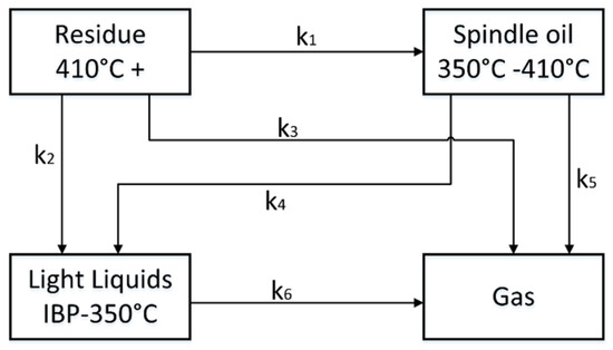
Figure 2.
Four-lump system with six monomolecular, irreversible reactions. IBP means initial boiling point higher than 0 °C and Gas is specified by incondensable at 0 °C.
For a reaction scheme of pyrolysis containing four lumps, four mass balances have to be computed. Additionally, the assumption of irreversible reactions is made to reduce the complexity further. This decreases the reaction pathways to six possibilities as shown in Figure 2. The radical character of the reaction system is neglected, and no recombination reactions are considered in the model. The six reactions (k1–k6) are described by the Arrhenius law to consider the temperature dependency,
in Equation (1) k is the reaction rate, A the Arrhenius constant, EA the activation energy, R the ideal gas constant, T the temperature and i the indices of the reactions 1 to 6. As mentioned before, the residence time cannot be determined directly, so there is no possibility to draw an Arrhenius plot. Hence the two parameters activation energy EA,i and the Arrhenuis constant Ai are unknown for each specified reaction i. Consequently, in this four-lump system 2 × 6 = 12 unknown parameters have to be obtained. For a further simplification of the model, a reaction order of 1 is assumed. Otherwise the unknown parameters would increase computational effort drastically. Finally, the model consists of a four-lump system with six monomolecular, irreversible, first order reactions with twelve unknown parameters.
Solving a problem like this requires a nonlinear regression solver. Such solvers are implemented for instance in Matlab and enable to find local and global minima for fitting the model to the measured data of the pilot plant.
As a precondition for the modeling of the plastic pyrolysis, the cracking behavior of the carrier fluid has to be investigated more in detail. For that, the composition of the carrier medium is required, which is obtained with the same analytic and distillation method as for the products. Based on the obtained boiling curve, the carrier fluid can be integrated in the four-lump system. So, most of the carrier medium is classified as “Residue”, but it also partly contains the boiling cuts of “Spindle oil” and “Light Liquids”. This composition is used for the starting conditions of the model. As already mentioned, test campaigns with the pure carrier fluid are performed and the reaction model like shown in Figure 2 is determined.
Subsequently, test runs with a certain plastic type are used to evaluate the thermal degradation of this plastic. The basic approach is the same as for the carrier fluid, but the plastic model needs an adaptation to insert the plastic into the four-lump model. So, an additional lump “Plastic” is linked to the heavy lump. The heavy lump is now called “Wax” (but has the same definition as “Residue”), the other lumps are named the same, “Spindle oil “(SO), “Light Liquids” (LL) and “Gas”, but are indexed with p for plastic. The lumped model for the plastic pyrolysis is shown in Figure 3.
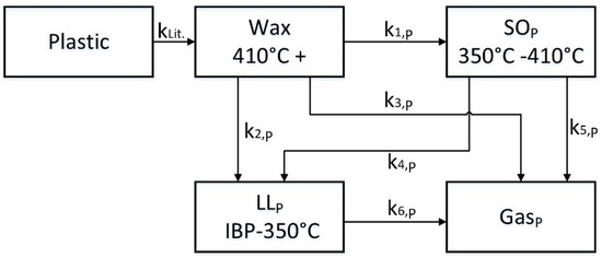
Figure 3.
5-lump model for the plastic pyrolysis with six monomolecular, irreversible, first order reactions and one starting reaction of the plastic degradation.
The six reaction rates ki,P of the five-lump model for plastic can be determined the same way as described before, just with the difference that the fraction of carrier fluid in the mixture is being calculated with the already determined four-lump model of the carrier fluid. The initial reaction kLit. cannot be evaluated in this pilot plant, because the conversion of the plastic needs to be very high (estimated 90–100%), in order to avoid blockage of the small pipes. Therefore, the already determined kinetics for different plastic types from literature are used to describe this first degradation step. Thermogravimetric analytics are suited well to predict the pyrolysis to gaseous components, so overall first order, degradation reactions are used like that described in [15,16,17]. In the Lumped Kinetic Model, the plastic is cracked down to a liquid wax phase described by the kinetics derived from TGA experiments (kLit.). Based on the given six pseudo reactions ki,P, the lumps react in a way which meet the measured mass fractions of the lumps.
2.2.2. Reactor Model
Based on the lumped kinetic model which represents the chemistry and kinetics of the cracking in the reactor, an overall reactor model is also developed. This model is based on the assumption of a plug flow reactor, whereas the mass balances can be constituted with deployed reaction rates as shown in Equations (2)–(6) for the lump system shown in Figure 3,
in the mass balances c describes the mass fraction of the respective lump, z is the reactor length, w is the local flow velocity of the whole stream (gas and liquid) and nLit. is the order of reaction for the used TGA degradation reaction of the plastic. It is assumed that all lumps (gas and liquid) move in the same velocity w, so there is no slip.
Additionally, a heat balance is integrated to evaluate the temperature profile over the reactor length (Equation (7)) because there is just six temperature measurements at the reactor wall,
whereas T is the local temperature, ρ is the density of the local mixture, cp is the heat capacity of the local mixture, kthermal is the local heat transfer coefficient, TW is the local wall temperature measured in the sand bath, d is the inner diameter of the reactor pipe and H is defined by Equation (8),
in Equation (8), Hr is the standard reaction enthalpy per mole change, MM is the mean molecular mass of the respective lump, Hmelt is the melting energy of the plastic by passing by the melting temperature and HV is calculated of the vaporizing fraction (vf) of the species respectively multiplied with the respective heat of evaporation (HVap) (Equation (9)),
Hr has been calculated out of the average paraffinic, olefinic and naphthenic composition of the cracking production. If a big paraffinic molecule split into two molecules, there are two possibilities:
- High Paraffin → Paraffin + Olefin
- High Paraffin → Paraffin + Naphthene
For each reaction, the enthalpies calculated of the heat of formations do not differ very much, independently how big the broken parts are as long the C and H balance is respected. The reaction enthalpies to paraffins and olefins is averaged to 76,232 kJ/mol and these to paraffins and naphthene is averaged to 57,101 kJ/mol. The mean distribution of olefins and naphthenes is 17:3, accordingly Hr is determined by 73,289 kJ/mol.
The last unknown factor of the heat balance is kthermal. To evaluate the heat transfer coefficient equations of the “VDI Wärmeatlas” [28] are used. Due to the complex construction of the plant, the reactors have different sections:
- Horizontal pipes
- ○
- One-phase flow [28] (Ga)
- ○
- Two-phase flow [28] (Hbb)
- Vertical up streamed pipes [28] (Hbb)
- Vertical down streamed pipes [28] (Hbb)
- Up streamed coils [28] (GC)
- Down streamed coils [28] (GC)
The length of all these sections is measured for all different reactor setup used. Moreover, in all sections one phase flow (only liquid) or two-phase flow may occur. For all these cases, suitable equations are available in [28] to calculate the heat transfer coefficient.
The coupled differential equation system has to be solved simultaneously, which is performed with Matlab. The solver calculates the reactor with the finite-element method discretely, whereas the minimal step size is one centimeter (Figure 4). Each discrete element is computed at constant conditions and the input is the starting values of the educt or the results of the previous element.

Figure 4.
Sketch of the discrete calculation of the tubular reactor with a finite-element method.
Finally, the kinetic data fitted to this model are determined with the nonlinear fitting tool. In this study, Matlab is used, which can calculate the model with the data By using reasonable starting points from previous models or from the literature [15,15,20,21,22,23], the model is calculated with random or algorithmic specified values until a local or global minimum is found by the method of least squares.
3. Results
This section reports the results for the pure carrier fluid, polypropylene, low density and high-density polyethylene, and compares the experimental results with the model. An overview of main test runs is given in Table 2. The main input parameters, such as mass fraction of plastic and carrier fluid, the mean reactor temperature, the pressure and the flow are shown. Additionally, the calculated residence time of the reaction medium above 400 °C and the conversion referring to the lump “Residue” are inserted in Table 2.
Table 2.
Exemplary test runs performed in the pilot plant. The total number of test runs was 67.
The pressure, reactor length, temperature of the sand baths and the flow rate are the main input data for the model. Additionally, the starting conditions have to be defined at the reactor inlet: The starting temperature, the composition of the carrier fluid and the mass fractions of plastic and carrier fluid. Then, the model calculates each discrete element of the reactor with starting kinetic values. After the calculation, the Optimization Toolbox of Matlab compares the calculated yields and the measured ones and changes the kinetic data for a new calculation. This is done until a minimum mean squared error between measured and modeled yields is found. An overview of the obtained values for the kinetic parameters is shown in Table 3. For the carrier fluid all six reactions take place and need to be formulated. This is due to the fact that the starting composition of the carrier fluid already contains the lumps, “Residue”, “Spindle oil” and “Light Liquids” (Figure 2). In order to obtain a reasonable fit, all lumps of the carrier fluid have to react. Contrary, kinetics of the plastics behaves differently. In a first attempt, also six reactions have been assumed, as shown in Figure 3. However, just three reactions are sufficient to describe the system, and to find a global minimum to fit all measured yields. All other reaction rates can be neglected (ki set to zero). In case of LDPE the conversion to products is very low and just the reaction k2 producing small amounts of “Light Liquids” is sufficient to model the measured yields. HDPE behaves like LDPE just with an additional reaction k6 to produce some “Gas” (Table 3).
Table 3.
Determined Arrhenius constants “A” and Activation Energies” EA” of the plastic pyrolysis in the pilot plant.
Additionally, parameters like the calculated flow velocity, temperature and vapor phase in any element can be exported from the model. With these data, the residence time of each test run can be obtained and the calculated temperature and concentration trends over length or time can be drawn. The corresponding legend is shown in Figure 5 and the trends are shown in Figure 6 and Figure 7.
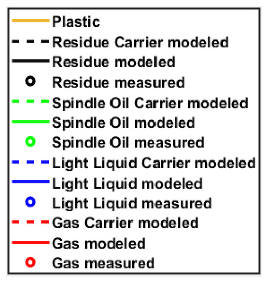
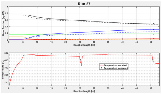
Figure 6.
Trends of mass fraction of the lumps and the temperatures over the reactor length for test run 27 with 10% PP.
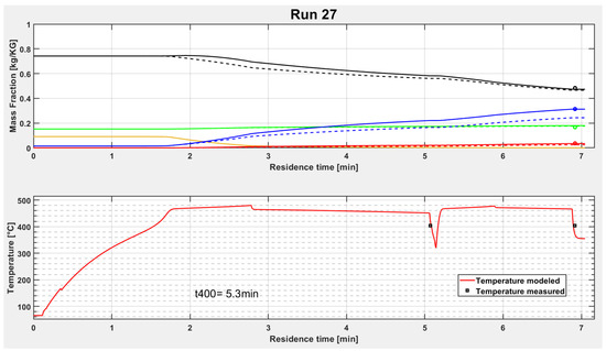
Figure 7.
Trends of mass fraction of the lumps and the temperatures over the time for test run 27 with 10% PP. The residence time with temperatures higher than 400 °C is 5.3 min for this test run.
It can be seen in Figure 6 and Figure 7 that PP cracks very fast at a certain temperature and completely converts to “Wax”. Then the light product fractions are increasing during the reactor while the “Residue” and the “Wax” are decreasing. The second plot in Figure 6 is the temperature trend. It increases also very fast after entering in the reactor. The medium temperature reaches the temperature of the sand bath nearly after five meter reactor length. After about 25 m, the first sand bath is passed and a short pipe section outside of the sand bath with a temperature measurement follows. A sharp temperature decrease can be seen clearly in the diagram. Then, the second sand bath begins and the temperature reaches again the hot equilibrium temperature.
Both tubular reactors in the sand baths have the same length of about 25 m in test run 27. However, the residence time in both sand baths are different, which can be derived from the temperature trend in Figure 7. The second sand bath has a residence time shorter than two minutes, whereas the first sand bath has more than three minutes residence time. This is due to the decrease of density of the medium, caused by produced gases and other light products, which results in higher flow velocities.
Furthermore, it can be seen that the modelled curves fit the measurement points quite well in test run 27. To determine the accuracy of the model, the next subchapters show deviation plots obtained for the different feedstocks investigated.
3.1. Carrier Fluid
At first the test runs with pure carrier fluids are evaluated. The carrier fluid contains nearly 10% of “Light Liquids” and after the pyrolysis more than 65% of “Light Liquids” can be measured. The deviations of the modeled and measured values are shown in Figure 8. The simple four lump model works very well for the carrier fluid pyrolysis, which can be derived from the low deviations to the diagonal line and also from the uniform distribution around the diagonal. There is just one outlier, which is also the only test run with a very high conversion. Hence, there is the indication that the model predicts well under mild pyrolysis conditions with a “Light Liquid” yield between 10 to 45%.
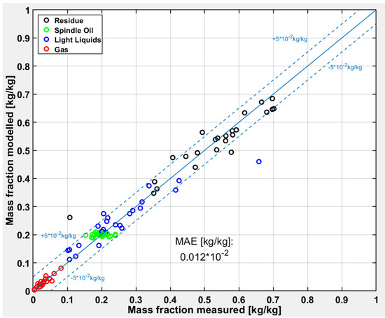
Figure 8.
Deviation of the modeled and measured values of the test runs with pure carrier fluid. “MAE” is the mean absolute error of the optimization of 0.01 × 10⁻² kg/kg. The dashed lines show the 10% deviation.
3.2. Polypropylene (PP)
Figure 9 shows the deviations between measured and modeled results for the test runs with PP. PP cracks at lower temperatures than the other plastic types studied in this work [8], which is confirmed by yields lower than 50% for the “Residue” fraction, except for one test run. Furthermore, the share of the “Residue” fraction is overpredicted from the model, contrariwise the share of the “Light Liquids” fraction is underpredicted.
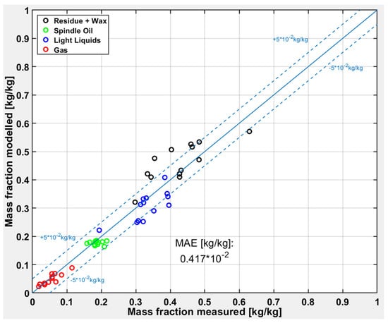
Figure 9.
Deviation of the modeled and measured values of the test runs with carrier fluid and PP. “MAE” is the mean absolute error of the optimization of 0.42 × 10⁻² kg/kg. The dashed lines show the 10% deviation.
3.3. Low Density Polyethylene (LDPE)
Figure 10 compares the test runs with LDPE with the model. The “Light Liquids” fraction is uniformly distributed which indicates a good fit, However, the “Spindle oil” fraction is overpredicted, even there is no reaction to produce “Spindle oil” (compare with Table 3). Consequently, the “Spindle Oil” fraction originates from the carrier fluid which indicates that there is a strong interaction between carrier fluid and LDPE. Additionally, the “Gas” lump has a uniform, but a high relative variance.
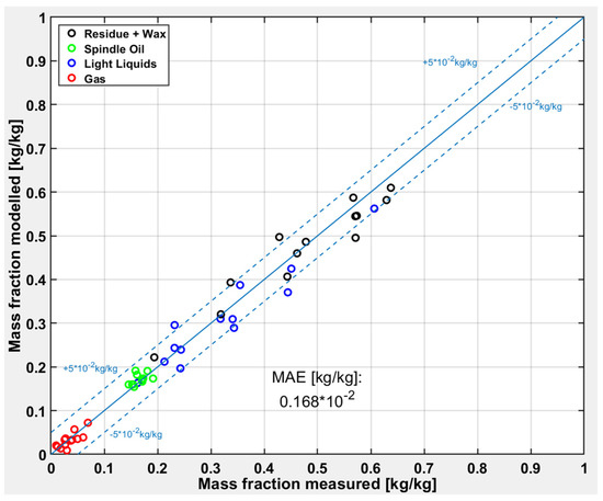
Figure 10.
Deviation of the modeled and measured values of the test runs with carrier fluid and LDPE. “MAE” is the mean absolute error of the optimization of 0.17 × 10⁻² kg/kg. The dashed lines show the 10% deviation.
3.4. High Density Polyethylene (HDPE)
The determined kinetic data for HDPE shows irregularities. At low conversions, the “Residue” lump is underpredicted, whereas the “Light Liquid” lump is overpredicted as shown in Figure 11. As well as in the LDPE kinetic the “Spindle oil” lump is overpredicted without having a “Spindle oil” producing reaction pathway in the plastic decomposition, and the “Gas” lump is slightly underpredicted.
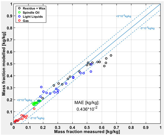
Figure 11.
Deviation of the modeled and measured values of the test runs with carrier fluid and HDPE. “MAE” is the mean absolute error of the optimization of 0.44 × 10⁻² kg/kg. The dashed lines show the 10% deviation.
4. Discussion
As shown in the previous chapter, the simple lump models provide a good agreement with the measured data from the pilot plant, especially the carrier fluid can be predicted with sufficient accuracy. The carrier fluid has a significant impact on the pyrolysis, although the reaction rates are lower than those of plastics, as shown in Table 4. Furthermore, the expected trends can be well modeled, whereas following order: PP > LDPE > HDPE for the reaction rates are expected from literature [22]. This is confirmed by the reactions rates for a given temperature producing “Light Liquids” via reactions path k2.
Table 4.
Reaction rates at 460 °C of all determined reactions and the used plastic decomposition reactions “kLit.” from [15].
The kinetic values for the plastic degradation reaction kLit. (Table 3) are taken from [15]. Also, the kinetic values of the carrier fluid, obtained by the model calculation are in a similar order of magnitude, which is also confirmed by the activation energy of around 200 kJ/mol. The calculated activation energies of the reaction paths involved in the PP pyrolysis fit well to literature, the lowest activation energy is 80 kJ/mol for the reaction from “Wax” to “Spindle oil” [5,8,16,17]. However, the calculated activation energy of 700 kJ/mol for reaction path k2 for LDPE and HDPE exceed the range of literature, even to those in comparison to oils [24]. Activation energies of oil cracking are in a frame of 50 to 500 kJ/mol [23]. The reason for this deviation can be assigned to the comparatively low product yields of “Light Liquids”, which can only be confirmed in test runs with higher temperatures. Further, test runs with increased temperatures and higher conversions need to be performed to receive more detailed data.
However, some differences can be seen between the kinetic data of PP and HDPE in Figure 9 and Figure 11, respectively. In the case of PP, the “Light Liquids” lump is underpredicted, although the total plastic feed is depolymerized, and its resulting “Wax” is also converted with the other product lumps completely. This indicates that there is an interaction between the carrier fluid and the plastic pyrolysis, which is not yet considered in the model. Hence, PP increases the outcome of products of the co-pyrolysis.
Contrariwise, the kinetic data of HDPE underpredicts the “Residue” lump at low conversions. Again, the HDPE is fully decomposed, and the produced “Light Liquids” lump is not originating 2 “Residue” lump is underpredicted, what indicates an interaction of the co-pyrolysis, in which the degradation of the carrier fluid is inhibited, or the carrier fluid produces a high boiling (410+ °C) product instead of a “Light Liquids” lump together with HDPE.
Additionally, the lump “Spindle oil” remains on the same level in the model, resulting in a horizontal trend in Figure 8 and Figure 9. “Spindle Oil” is also not produced from LDPE and HDPE, but is nevertheless overpredicted. Consequently, the reaction mechanism of producing “Spindle Oil” is not sufficiently considered in the model, but this has just a low effect on the variance.
5. Conclusions
The provided lumping approach reduces the complexity of the chemical reaction system significantly by reducing the interacting components, this drastically lowers the analytical and computational effort for the model calculation. In contrast, in order to the common practice operating mostly with TGA measurements, this model can investigate the decomposition processes in a tubular reactor by adding consecutive reactions. The reactor calculation can describe the effect of evaporation and the resulting flow regimes inside the reactor pipe. Also, the complexity of the reaction model is still low (just four lumps), the kinetic data for a satisfying description of the pyrolysis of PP, LDPE and HDPE are found. Simultaneously to the chemical reactions, the heat transfer is described analogously to flow boiling which results in reasonable temperature trends. Due to the temperatures, evaporation, condensation and chemical reactions the density of the reaction medium changes over the whole reactor length, but the model considers all these mechanisms, and thus, provides a reasonable residence time of reaction mixtures in the reactor. Furthermore, the often-used Arrhenius approach obviously describes the temperature dependency sufficiently.
Under the used mild cracking conditions, polyethylene has imperfect conversion towards the products lumps “Spindle oil”, “Light Liquids” and “Gas”. In particular, the “Spindle oil” lump seems to have different chemical mechanisms, interacting with the carrier fluid. Also PP shows interactions with the carrier fluid, in which the conversion to “Light Liquids” is enhanced.
To generate a more precise prediction, these interactions of the carrier fluid and the plastics should be introduced. Moreover, the formation of coke should be included, which could be inserted with a C/H balance to the system.
However, this lumped kinetic model achieve a sufficient description of the process and hence it is already used in a plant simulation to provide data for an upscale.
Author Contributions
Conceptualization, A.E.L. and T.S.; methodology, A.E.L.; software, A.E.L.; validation, A.E.L. and T.S.; formal analysis, A.E.L.; investigation, A.E.L.; resources, A.E.L. and W.H.; data curation, A.E.L. and T.S.; writing—original draft preparation, A.E.L.; writing—review and editing, A.E.L.; visualization, A.E.L. and T.S.; supervision, M.L. project administration, W.H. All authors have read and agreed to the published version of the manuscript.
Funding
This research received no external funding.
Data Availability Statement
Restrictions apply to the availability of these data. Data was obtained from OMV Downstream GmbH and are available from the authors with the permission of OMV Downstream GmbH.
Conflicts of Interest
The authors declare no conflict of interest.
References
- Plasticseurope. Available online: https://www.plasticseurope.org/ (accessed on 20 October 2020).
- European Commission. Eine Europäische Strategie für Kunststoffe in der Kreislaufwirtschaft. 2018. Available online: https://eur-lex.europa.eu/resource.html?uri=cellar:2df5d1d2-fac7-11e7-b8f5-01aa75ed71a1.0002.02/DOC_3&format=PDF (accessed on 8 August 2018).
- Europäische Union. Richtlinie (EU) 2018/ des Europäischen Parlaments und des Rates vom 30 Mai 2018 zur Änderung der Richtlinie 2008/98/EG über Abfälle. 2018. Available online: https://eur-lex.europa.eu/legal-content/DE/TXT/?uri=CELEX:32018L0852 (accessed on 8 August 2018).
- Quicker, P. Evaluation of Recent Developments Regarding Alternative Thermal Waste Treatment with a Focus on Depolymerisation Processes. 2019. Available online: https://www.vivis.de/wp-content/uploads/WM9/2019_WM_359-370_Quicker.pdf (accessed on 25 November 2020).
- Aguado, J.; Serrano, D.P. Feedstock Recycling of Plastic Wastes; Royal Society of Chemistry: Cambridge, UK, 1999. [Google Scholar]
- Al-Salem, S.M.; Antelava, A.; Constantinou, A.; Manos, G.; Dutta, A. A review on thermal and catalytic pyrolysis of plastic solid waste (PSW). J. Environ. Manag. 2017, 197, 177–198. [Google Scholar] [CrossRef] [PubMed]
- Anuar Sharuddin, S.D.; Abnisa, F.; Wan Daud, W.M.; Aroua, M.K. A review on pyrolysis of plastic wastes. Energy Convers. Manag. 2016, 115, 308–326. [Google Scholar] [CrossRef]
- Scheirs, J.; Kaminsky, W. (Eds.) Feedstock recycling and Pyrolysis of Waste Plastics: Converting Waste Plastics into Diesel and Other Fuels; John Wiley & Sons Ltd.: Chichester, UK, 2006. [Google Scholar]
- Vogel, J.; Krüger, F.; Fabian, M. Chemisches Recycling. Hintergrund July 2020. Available online: https://www.umweltbundesamt.de/sites/default/files/medien/1410/publikationen/2020-07-17_hgp_chemisches-recycling_online.pdf (accessed on 24 August 2020).
- Lederer, C.; Lehner, M. Development of an upscalable process for polyolefins and other post-consumer plastic fractions via solvent-based depolymerization. In Proceedings of the 7th International Symposium on Feedstock Recycling of Polymeric Materials (7th ISFR 2013), New Delhi, India, 23–26 October 2013. [Google Scholar]
- Schubert, T.; Lechleitner, A.; Lehner, M.; Hofer, W. 4-Lump kinetic model of the co-pyrolysis of LDPE and a heavy petroleum fraction. Fuel 2020, 262, 116597. [Google Scholar] [CrossRef]
- Brown, M.E. Introduction to Thermal Analysis: Techniques and Applications; Springer: Dordrecht, The Netherlands, 2001. [Google Scholar]
- Kiang, J.K.Y.; Uden, P.C.; Chien, J.C.W. Polymer Reactions—Part VII: Thermal Pyrolysis of Polypropylene. Polym. Degrad. Stab. 1980, 2, 113–127. [Google Scholar] [CrossRef]
- Bockhorn, H.; Hornung, A.; Hornung, U. Mechanisms and kinetics of thermal decomposition of plastics from isothermal and dynamic measurements. J. Anal. Appl. Pyrolysis 1999, 50, 77–101. [Google Scholar] [CrossRef]
- Westerhout, R.W.; Waanders, J.; Kuipers, J.A.; Swaaij, W.P. Kinetics of the Low Temperature Pyrolysis of Polyethene, Polypropene, and Polystyrene, Modeling, Experimental Determination, and Comparison with Literature Models and Data. Industiral Eng. Chem. Res. 1997, 36, 1955–1964. [Google Scholar] [CrossRef]
- Bockhorn, H.; Hornung, A.; Hornung, U.; Schawaller, D. Kinetic study on the thermal degradation of polypropylene and polyethylene. J. Anal. Appl. Pyrolysis 1999, 48, 93–109. [Google Scholar] [CrossRef]
- Aboulkas, A.; El harfi, K.; El Bouadili, A. Thermal degradation behaviors of polyethylene and polypropylene. Part I: Pyrolysis kinetics and mechanisms. Energy Convers. Manag. 2010, 51, 1363–1369. [Google Scholar] [CrossRef]
- Tsuchiya, Y.; Sumi, K. Thermal decomposition products of polypropylene. J. Polym. Sci. Part. A-1 1969, 7, 1599–1607. [Google Scholar] [CrossRef]
- Buxbaum, L.H. The Degradation of Poly(ethylene terephthalate). Angew. Chem. Int. Ed. Engl. 1968, 7, 182–190. [Google Scholar] [CrossRef]
- Schubert, T.; Lehner, M.; Hofer, W. Experimental and modeling approach of LDPE thermal cracking for feedstock recycling. In Proceedings of the 9th International Symposium on Feedstock Recycling of Polymeric Materials (9th ISFR 2017), Ostrava, Czech Republic, 10–13 July 2017. [Google Scholar]
- Schubert, T.; Lehner, M.; Karner, T.; Hofer, W.; Lechleitner, A. Influence of reaction pressure on co-pyrolysis of LDPE and a heavy petroleum fraction. Fuel Process. Technol. 2019, 193, 204–211. [Google Scholar] [CrossRef]
- Singh, J. (Ed.) Feedstock Recycling and Pyrolysis of Waste Plastics: Converting Waste Plastics into Diesel and Other Fuels; Wiley & Sons: Chichester, UK, 2006. [Google Scholar]
- Singh, J.; Kumar, M.M.; Saxena, A.K.; Kumar, S. Reaction pathways and product yields in mild thermal cracking of vacuum residues: A multi-lump kinetic model. Chem. Eng. J. 2005, 108, 239–248. [Google Scholar] [CrossRef]
- Del Bianco, A.; Panariti, N.; Anelli, M.; Beltrame, P.L.; Carniti, P. Thermal cracking of petroleum residues. Fuel 1993, 72, 75–80. [Google Scholar] [CrossRef]
- Kuo, J.C.; Wei, J. Lumping Analysis in Monomolecular Reaction Systems. Analysis of Approximately Lumpable System. Ind. Eng. Chem. Fund. 1969, 8, 124–133. [Google Scholar] [CrossRef]
- Wei, J.; Kuo, J.C. Lumping Analysis in Monomolecular Reaction Systems. Analysis of the Exactly Lumpable System. Ind. Eng. Chem. Fund. 1969, 8, 114–123. [Google Scholar] [CrossRef]
- Schubert, T. Experimental Investigation and Modeling of a Polyolefin Pyrolysis Process; Montanuniversitaet: Leoben, Austria, 2018. [Google Scholar]
- Kabelac, S. (Ed.) VDI-Wärmeatlas: [Berechnungsunterlagen für Druckverlust, Wärme- und Stoffübergang]; Springer: Berlin/Heidelberg, Germany, 2006. [Google Scholar]


Publisher’s Note: MDPI stays neutral with regard to jurisdictional claims in published maps and institutional affiliations. |
© 2020 by the authors. Licensee MDPI, Basel, Switzerland. This article is an open access article distributed under the terms and conditions of the Creative Commons Attribution (CC BY) license (http://creativecommons.org/licenses/by/4.0/).