Abstract
Energy flexibility in regulated users is examined as a structural property of demand, assessed through variability and disorder metrics derived from smart metering data. Using the coefficient of variation and normalized entropy, the analysis reveals stable routines during weekdays and greater heterogeneity in transitional periods such as evenings and weekends. Non-negative matrix factorization (NMF) is applied to extract latent user pro-files, which are subsequently clustered to uncover representative trajectories of consumption. Groups with bimodal or extended load distributions emerge as the most adaptable, highlighting the role of latent profiling in identifying flexibility potential. Simulations of partial load redistribution demonstrate that, while individual savings remain modest, aggregated benefits and improvements in reliability indicators (SAIDI, SAIFI, ENS) are significant. These findings confirm that flexibility is unevenly distributed across users and time, and that its quantification provides a strategic foundation for differentiated demand response schemes and the design of resilient, user-oriented energy systems.
1. Introduction
The sustained growth of energy demand and the transition towards renewable sources have intensified the need to improve efficiency and enable smart management of electricity consumption. Understanding consumption patterns is essential to optimize resource use, reduce emissions, and ensure the stability of the power system [1,2,3]. The digitalization of the sector has facilitated the adoption of advanced metering infrastructures (AMI), which provide high-resolution temporal data and enable more precise demand control [4,5,6,7]. However, the effective use of this information remains a challenge due to the complexity of consumption profiles and the variability introduced by renewable sources. One of the main challenges in smart grids is user characterization, since understanding consumption habits allows the design of personalized energy management strategies. Techniques such as K-means, SOM, and hierarchical clustering have been applied to segment consumers according to their demand profiles [8,9,10], although their integration with demand response schemes remains limited.
In this context, the quantitative characterization of consumption patterns plays a key role in identifying profiles with high variability and greater potential for energy flexibility. Metrics such as Shannon entropy, which evaluates complexity and uncertainty in time series, and the coefficient of variation (CV), which quantifies the relative dispersion of the signal, have proven useful for this type of analysis [11,12,13,14,15,16]. This study proposes an approach based on these metrics to evaluate variability, stability, and complexity in electricity consumption. Identifying users with high flexibility potential is crucial to improve system stability and facilitate the integration of intermittent renewable energies [17,18,19]. The analysis is complemented with visualizations that reveal significant temporal dynamics and provide inputs for energy planning. Although multiple clustering techniques exist to characterize consumption profiles, many require strong assumptions about group shape and separation, which may limit their applicability in contexts with high dispersion and overlap among users [20,21].
In this study, an alternative approach based on non-negative matrix factorization (NMF) is adopted, which identifies latent components from weighted combinations of metrics such as entropy and coefficient of variation [11,22,23]. This approach does not aim to directly segment users, but rather to reveal thematic profiles that synthesize recur-rent patterns in the dataset. By working with latent representations, NMF facilitates the functional interpretation of profiles and allows their temporal stability to be evaluated using measures such as cosine similarity [20,24]. This strategy is particularly useful for characterizing energy flexibility potential, by identifying users with structured or dispersed behaviors according to their metric composition [1,25].
The main contribution of this study is oriented towards utilities and aggregators, providing methodological tools to identify flexibility potential at the user level and integrate it into system-level planning. By linking consumption variability and entropy metrics with latent profiling, the approach highlights how demand-side flexibility can improve reliability indicators (SAIDI, SAIFI, ENS) and support the design of resilient, user-oriented energy systems.
2. Materials and Methods
This section describes the methodological framework applied to characterize variability and disorder in regulated electricity consumption, as well as the procedures for clustering and simulation of economic and reliability impacts. All steps were implemented in Python 3.13.2 to ensure reproducibility.
2.1. Data Collection and Preprocessing
The dataset was provided from Colombia and comprises regulated residential, commercial, industrial, and official users. The socioeconomic composition is represented by strata E1–E6, consistent with the Colombian classification system. Geographically, the data span 25 municipalities across Bogotá D.C., Cundinamarca, and Tolima, including major urban centers. This scope ensures representation of diverse urban and peri-urban consumption patterns within the central region of Colombia.
Hourly electricity consumption records were obtained from these users and organized by year, month, day type, and user identifier. Each dataset was structured into 24 h series per user, enabling the construction of hourly distributions for subsequent statistical analysis [26]. The general organization of the data is summarized in Table 1. To ensure statistical validity, a preprocessing workflow was implemented as shown in Figure 1. The main steps were:

Table 1.
Summary of the structure of the energy data used.
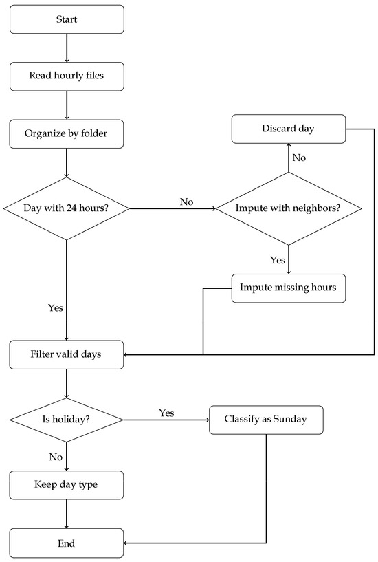
Figure 1.
Flow diagram of hourly data preprocessing per user.
- Structured folder loading: Files were organized by month and day of the week, allowing segmentation of the analysis with a clear temporal basis.
- Neighbor interpolation: Neighbor interpolation was applied under the assumption of temporal smoothness in electricity demand. This assumption is particularly appropriate for residential users, where household consumption typically evolves gradually throughout the day. For other regulated user categories, the same criterion was adopted to ensure consistency in preprocessing and preserve realistic load dynamics at the hourly resolution. Sudden discontinuities are rare at the hourly resolution considered, so imputing missing values from adjacent hours preserves the realistic dynamics of residential load profiles [4,6]. If a user presented fewer than 24 h in a day, missing values were imputed using the average of neighboring hours (previous and next). If imputation was not possible, the day was discarded [4,6].
- Filtering of valid days: Only days in which the 24 h series could be reliably recon-structed, either complete or imputed, were processed.
- Automatic holiday detection: The holidays library was used to identify Colombian holidays. If a day was a holiday, it was classified as equivalent to Sunday, ensuring accurate grouping by day type [20,21].
After filtering valid daily profiles, the data were aggregated by day type within each month. For example, all Mondays of February were grouped together for each user, and hourly consumption values across those days were used to construct distributions at each hour (0–23). These distributions served as the basis for computing the coefficient of variation (CV) and normalized entropy per hour and day type. This procedure ensured that the metrics reflected consistent intra-day variability across comparable temporal segments, resulting in 336 variables per user (24 h × 7 day types × 2 metrics).
It is important to note that the preprocessing workflow involved two levels of filtering. The first stage operated at the daily level, removing incomplete or non-imputable records before the computation of variability and entropy metrics (Figure 1). Once metrics were computed, a second stage was applied at the user level, requiring complete hourly profiles across all day types within a month (336 variables). Any missing value led to exclusion, producing a more substantial reduction in the sample size (Figure 2). This consolidated dataset served as the input for subsequent clustering and latent profile extraction.
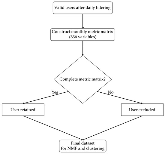
Figure 2.
Second filtering stage within preprocessing: construction of monthly metric matrices and exclusion of users with incomplete profiles after metric computation.
2.2. User Retention Across Preprocessing Stages
To ensure transparency in the preprocessing workflow, the number of users retained was reported explicitly by month and by filtering stage.
Table 2 summarizes the evolution of the dataset across the three stages: (i) initial users, (ii) users remaining after the first filter (removal of incomplete or non-imputable daily records), (iii) users retained after the second filter (requirement of complete hourly profiles across all day types within a month), and additionally reports the number of discarded daily records per month.
Table 2.
Monthly user counts and discarded daily records at each preprocessing stage (2017–2020).
This integrated view provides transparency on both user retention and the temporal distribution of missing or invalid daily profiles.
2.3. Metrics for Variability and Complexity
Variability and complexity in electricity consumption were characterized using two statistical measures: the coefficient of variation (CV) and normalized Shannon entropy. For each user, hourly consumption distributions were constructed by aggregating all days of the same type within a month (e.g., all Mondays in February). At each hour (0–23), the set of values across those days was used to compute variability and disorder. This procedure ensured that the metrics captured intra-day variability consistently across comparable temporal segments, resulting in 336 variables per user (24 h × 7 day types × 2 metrics). While both direct and bin-based formulations of normalized entropy were evaluated, the direct approach yielded values consistently above 0.98 with minimal variation, limiting interpretability (Figure 3). In contrast, bin-based rules (Freedman–Diaconis, Sturges, Scott) provided smoother and more informative distributions, aligning with the discrete nature of hourly consumption records. Although the overall patterns remained consistent across methods, Freedman–Diaconis produced slightly broader ranges and revealed distinctive behavior at one specific hour. Sturges and Scott yielded smoother curves, confirming that the observed trends are not artifacts of a single discretization scheme. The convergence of results across all binning rules demonstrates methodological robustness, ensuring that entropy-based measures capture genuine consumption dynamics rather than being driven by arbitrary parameter choices. Therefore, the bin-based normalized entropy was adopted as the main measure of disorder, offering clearer insights into users’ flexibility potential [11,13,14,15,16,27,28].
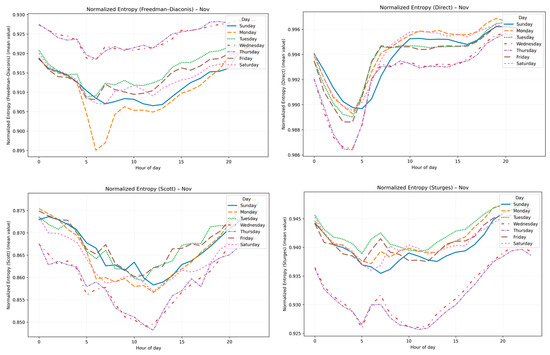
Figure 3.
Comparison of normalized entropy estimates: direct vs. bin-based rules (Freedman–Diaconis, Sturges, Scott).
- Coefficient of Variation (CV): Relative dispersion of hourly consumption, defined as:where σ is the standard deviation and µ the mean. High CV indicates greater variability in user demand [11,13,14].
- Normalized Shannon Entropy: To quantify disorder in consumption distributions, values were discretized into bins using the Freedman–Diaconis rule [15,16], which adapts bin width to the interquartile range and sample size:This avoids artificial inflation of entropy due to minor consumption variations. Entropy was then computed as:where k is the number of bins defined by the Freedman–Diaconis rule, and pj is the probability of consumption values falling into bin j, with and normalized by its maximum value:ensuring comparability across users and periods [11,12,28].
This normalization is justified because the maximum entropy for a discrete distribution with k bins occurs when all categories are equally probable, i.e., pj = 1/k for every j. Substituting into Equation (3) yields:
Thus, log2(k) represents the theoretical maximum entropy attainable under uniform distributions. Dividing by this value ensures that the normalized entropy Hnorm lies within the interval [0, 1], where 0 indicates complete order (all probability concentrated in one bin) and 1 indicates maximum disorder (uniform distribution across bins). This scaling guarantees comparability across users and periods, preventing artificial inflation of entropy values due to differences in discretization granularity. Continuous entropy estimators (e.g., kernel density or k-nearest neighbor approaches) were considered; however, these methods typically assume smooth underlying probability densities and require large sample sizes to mitigate estimation bias [15,16]. Given the limited number of daily observations available per hour and the inherently discrete nature of residential electricity consumption profiles, such assumptions are difficult to satisfy in practice. Consequently, bin-based Shannon entropy was adopted as a more robust and interpretable measure of disorder, as it provides stable estimates under small-sample conditions and facilitates consistent comparisons across users and time periods [11,12,20,21].
Together, CV and normalized entropy provided a robust characterization of variability and complexity, serving as the basis for subsequent clustering and latent profile extraction.
2.4. Clustering and Latent Profile Extraction
User-metric matrices were constructed with 336 variables per user (24 h × 7 days for both CV and normalized entropy). This high-dimensional representation was initially clustered using K-Means directly on the original matrix. However, the results were unsatisfactory according to clustering quality indices, showing redundancy among variables and dispersion in the representation space [8,20].
To address these limitations, Non-Negative Matrix Factorization (NMF) was applied to obtain latent profiles. Given a non-negative matrix X ∈ Rm×n, NMF seeks two non-negative matrices W and H such that:
where W ∈ Rm×r contains the latent representation of users, with each row describing the contribution of a user to the r profiles, and H ∈ Rr×n defines the latent profiles them-selves, with each row indicating the weight of the original variables in the corresponding profile [11,22,23].
Latent profiles (H): The thematic composition of each profile was analyzed to identify dominance of variability (CV) or dispersion (entropy). Temporal stability of these profiles was evaluated through cosine similarity:
which quantified the alignment between latent vectors across consecutive months [24]. Stable similarity values indicated that the latent structures preserved their internal composition over time.
User clusters (W): Subsequent clustering was performed on W using K-Means, with the optimal number of clusters determined by the elbow method. This step grouped users according to their contributions to the latent profiles, yielding interpretable segments. Cluster stability was assessed by tracking user assignments across months, confirming that the segmentation remained coherent and robust.
This combined approach—dimensionality reduction with NMF followed by clustering—yielded more coherent and stable groupings than direct segmentation on the original matrix, while also enabling the interpretation of both latent profiles and user clusters in terms of variability and complexity [8].
2.5. Simulation of Economic and Reliability Impacts
In order to evaluate the implications of user flexibility, simulation scenarios were defined combining economic and reliability perspectives [17,18,19,25].
Economic simulation: Although the dataset covers multiple municipalities across Bogotá D.C., Cundinamarca, and Tolima, the economic simulations adopted official tariff values for Bogotá in 2017, used as a representative benchmark due to their availability and regulatory relevance. Redistribution of 5%, 10% and 20% of peak-hour consumption was applied to latent functions B and D. Peak hours were defined as those exceeding 90% of the daily maximum, while valley hours were those below 70%. A simulated hourly tariff was constructed based on official values for Bogotá [29], with an average of 374.71 COP/kWh, penalization in peak hours (487.12 COP/kWh) and bonus in valley hours (299.77 COP/kWh) [29]. For international comparability, these values were also expressed in USD using the official exchange rate (TRM) published by the Banco de la República de Colombia. The TRM used corresponds to 20 January 2026, with 1 USD = 3700.05 COP [30]. Accordingly, the tariffs are equivalent to:
- Average tariff: 374.71 COP/kWh ≈ 0.101 USD/kWh
- Peak tariff: 487.12 COP/kWh ≈ 0.132 USD/kWh
- Valley tariff: 299.77 COP/kWh ≈ 0.081 USD/kWh
Monthly and annual savings were estimated by aggregating daily results, maintaining constant total daily consumption. The simulations were performed using consumption data from the year 2017, which served as the reference period for latent function characterization. Aggregated savings were calculated considering the number of users associated with each function in that year (7805 for Function B and 2369 for Function D, totaling 10,174 users).
2.6. Reliability Simulation
System reliability was assessed using indicators SAIDI, SAIFI and unsupplied energy (ENS) [1,7,19,31].
The simulation was parameterized to represent a sector equivalent to 1000 users. These users were distributed across the four trajectories (A, B, C, D) in proportion to the monthly average number of users observed in each trajectory, ensuring that the sector composition reflected the empirical structure of the dataset. Minor rounding adjustments were applied to guarantee that the total number of users summed exactly to 1000.
As an illustrative example, Table 3 shows the distribution of users across trajectories A–D for March 2017, extrapolated to a sector of 1000 users. This composition was used to construct the base sector curve and apply the redistribution scenarios presented in the graphical analysis.
Table 3.
Example of monthly user distribution (March 2017).
For each function, 30% of users were assumed to be affected during interruptions, consistent with the operational assumptions of the framework.
A nominal capacity limit of 0.36 MW was adopted, and critical hours were defined as those exceeding this limit, while safe hours corresponded to demand below 85% of capacity, representing a conservative operational margin.
Redistribution scenarios of 5%, 10%, and 20% of peak-hour load were applied exclusively to flexible functions (B and D), while rigid functions (A and C) remained unchanged. These percentages were selected to represent realistic ranges of demand-side participation, ensuring that the simulation captured both modest and ambitious flexibility contributions.
This parameterization provided the basis for the results presented in Section 3, where economic savings and reliability improvements are reported.
3. Results
The results are presented in four parts, reflecting the methodological stages described in Section 2. First, preliminary analyses of variability and complexity are reported, based on hourly series of the coefficient of variation (CV) and normalized Shannon entropy. Second, clustering outcomes are discussed, including direct application of K-Means on the original user–metric matrices and the improved segmentation obtained through Non-Negative Matrix Factorization (NMF). Third, the economic impacts of load redistribution are quantified under simulated hourly tariffs, highlighting the savings potential of flexible functions. Finally, reliability improvements are evaluated through indicators such as SAIDI, SAIFI, and unsupplied energy (ENS), demonstrating the operational benefits of user flexibility. This structure enables a progressive interpretation: from statistical characterization, to functional segmentation, and ultimately to the quantification of economic and reliability impacts.
3.1. Preliminary Analysis of Variability and Complexity
Hourly series of the coefficient of variation (CV) and normalized Shannon entropy were computed for each user, month, and day type. The aggregated curves reveal consistent patterns: weekdays from Tuesday to Friday exhibit high similarity, with correlations above 0.95, while Mondays, Saturdays, and Sundays show greater dispersion and amplitude. Entropy values peak between 21 h and 23 h, indicating heterogeneous evening behaviors, and reach minima between 5 h and 7 h, reflecting structured morning routines. The interpretation of these findings is that consumption stability is concentrated in mid-week days, whereas transitional days (Monday, Saturday, Sunday) present higher variability. This distinction suggests that flexibility potential is not uniformly distributed across the week: it is greater in days with dispersed or unpredictable behaviors, which can be targeted for demand response strategies. The experimental conclusion is that CV and entropy jointly provide a robust basis for identifying critical time windows and user groups with higher adaptability, thereby supporting the design of differentiated flexibility programs.
3.1.1. Patterns by Day of the Week (2017)
The aggregated hourly curves are shown in Figure 4 and Figure 5, which present the evolution of entropy and CV by day type and month. These plots confirm the compact clustering of mid-week days (Tuesday–Friday), while transitional days (Monday, Saturday, Sunday) exhibit dispersed and irregular structures.
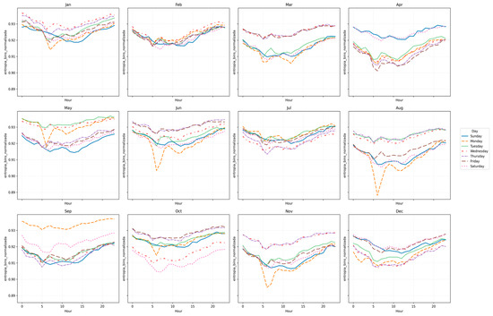
Figure 4.
FacetGrid of hourly curves for each day—Normalized Entropy Bins (2017).
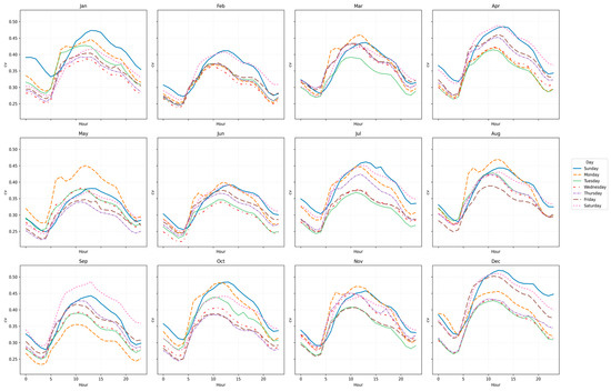
Figure 5.
FacetGrid of hourly curves for each day—CV (2017).
Complementary quantitative results are summarized in Table 4, which reports representative Pearson correlations and error metrics (MAE) between day types. These values confirm the high similarity between mid-week days, while transitional days show lower correlations.
Table 4.
Representative intra-month correlations (Entropy).
In addition, Table 5 lists representative maximum and minimum amplitudes per day and month. These values illustrate the general pattern observed across all months: high similarity between mid-week days, and greater variability in transitional days.
Table 5.
Representative hourly amplitudes of CV and entropy.
3.1.2. Temporal Evolution in 3D Surfaces (2017–2020)
Beyond the intra-annual analysis, three-dimensional surfaces were generated to capture the evolution of CV and entropy between 2017 and 2020. Figure 6 and Figure 7 show that CV exhibits a growing trend toward the last quarter of 2017 and a sustained increase across multiple hourly ranges in the full period. This behavior may be linked to demographic growth in Bogotá (reported by DANE) and the incorporation of new appliances and emerging technologies (e.g., solar panels, batteries, electric vehicles), which increase heterogeneity in consumption profiles.
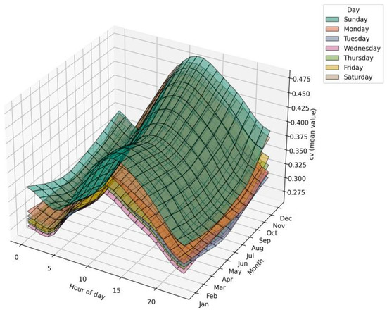
Figure 6.
Hourly surfaces of CV by day and month (2017).
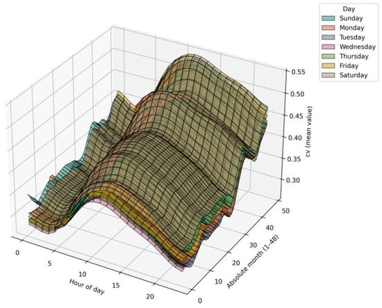
Figure 7.
Hourly surfaces of CV by day and month (2017–2020).
In contrast, entropy surfaces (Figure 8 and Figure 9) remain relatively stable across years, showing well-defined hourly patterns without significant increases in dispersion. This stability reflects the structural nature of entropy, which captures distributional complexity rather than magnitude, and is reinforced by the Freedman–Diaconis rule that adapts bin widths to data ranges without artificially inflating variability.
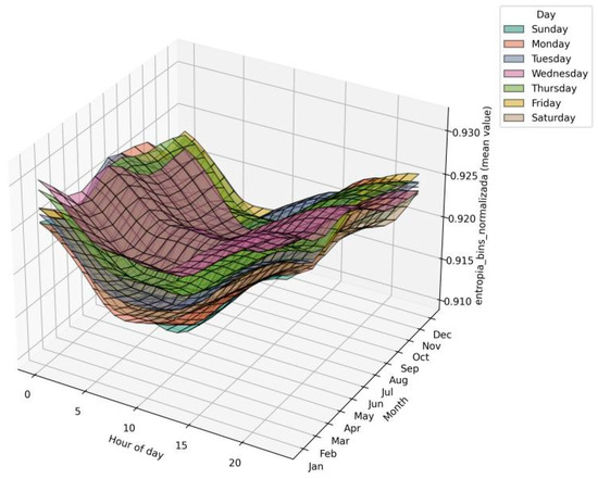
Figure 8.
Hourly surfaces of Normalized Entropy by Bins, by day and month (2017).
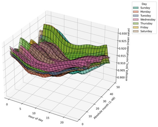
Figure 9.
Hourly surfaces of Normalized Entropy by Bins, by day and month (2017–2020).
Joint interpretation: The divergence between CV and entropy suggests that while CV reflects the intensification and variability of energy use, entropy remains robust against demographic or technological scaling. This reinforces its utility as a structural descriptor of consumption behavior, especially in contexts of urban expansion or residential transformation. Together, these results demonstrate that even relatively simple statistical metrics can reveal collective flexibility, supporting the need to advance toward user clustering techniques to identify differentiated consumption profiles and design targeted demand response strategies.
The stability of entropy across years indicates that, despite demographic growth or technological adoption, the relative distribution of consumption within the day remains consistent. Entropy is insensitive to absolute demand levels, focusing instead on how load is spread across hours. This makes it a structural descriptor: it captures the underlying organization of routines (morning peaks, evening peaks) rather than their intensity. In contrast, CV amplifies changes in magnitude, reflecting external drivers such as appliance penetration. Therefore, entropy stability justifies its interpretation as structural behavior, since it reveals persistent temporal organization in consumption patterns even under scaling effects.
3.2. Clustering Outcomes
To segment users according to their energy consumption patterns, clustering strategies were applied to monthly matrices constructed from hourly variables. Each matrix contains one row per user and 336 columns (24 h × 7 days × 2 metrics: CV and entropy). This structure captures temporal variability but introduces high dimensionality, which complicates direct segmentation. Table 6 illustrates the organization of this matrix.
Table 6.
Simplified structure of the user matrix (CV and entropy by hour and day).
3.2.1. Direct Clustering on the Original Matrix
As a first approach, K-Means was applied directly to the original matrix. The elbow method suggested k = 4 clusters (Figure 10), but the quality metrics were poor, with low separation and high internal dispersion. Table 7 summarizes the results for February 2017, representative of other months.
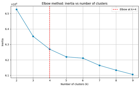
Figure 10.
Elbow method applied to the original matrix (February 2017).
Table 7.
Clustering quality metrics on the original matrix (February 2017).
These results show that direct clustering failed to capture consistent patterns, due to redundancy and noise in the high-dimensional space.
To further quantify redundancy in the original 336-variable matrix, a correlation analysis was conducted.
Across all months between 2017 and 2020, approximately 30–33% of variable pairs exhibited correlation coefficients above 0.8.
This confirms the presence of substantial redundancy among hourly and day-type features, supporting the conclusion that direct clustering failed due to the high-dimensional noise.
3.2.2. Dimensionality Reduction with NMF
To overcome these limitations, Non-Negative Matrix Factorization (NMF) was applied, decomposing the original matrix X into W (user compositions) and H (latent profiles). This representation is more compact and interpretable, allowing latent structures in consumption to be revealed. Subsequently, K-Means clustering was applied to W, yielding improved segmentation quality.
Daily, monthly and annual savings were then estimated by comparing base and flexible scenarios, maintaining constant total daily consumption. more compact and interpretable. K-Means was then applied to W, yielding improved clustering quality. Table 8 shows the evaluation for February 2017.
Table 8.
Evaluation of NMF + K-Means.
The dimensionality reduction rank r was selected based on quantitative clustering quality indices.
Specifically, the Silhouette index (measuring cohesion and separation), the Calinski-Harabasz index (compactness and separation), and the Davies-Bouldin index (cluster similarity and dispersion) were computed for different values of r.
For r = 2, the Silhouette index reached its maximum (0.49), the Calinski-Harabasz index was highest (38,468), and the Davies-Bouldin index was lowest (0.61), indicating compact and well-separated clusters.
Higher values of r (3 or 4) yielded poorer clustering quality (Silhouette = 0.33–0.32, Calinski-Harabasz decreased, Davies-Bouldin increased to 0.89–0.95), despite marginal improvements in reconstruction loss.
Therefore, r = 2 was adopted as the most parsimonious choice, balancing reconstruction accuracy with clustering quality and interpretability.
3.2.3. Latent Profile Characterization
Two latent profiles were identified:
- Profile 0: dominated by CV variables, representing users with high hourly variability.
- Profile 1: dominated by entropy variables, representing users with more distributed and stable consumption.
Figure 11 and Figure 12 illustrate the distribution of CV and entropy across latent profiles. To complement these visualizations, Table 9 summarizes representative values.
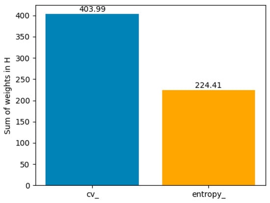
Figure 11.
Profile 0—distribution of weights (CV vs. entropy).
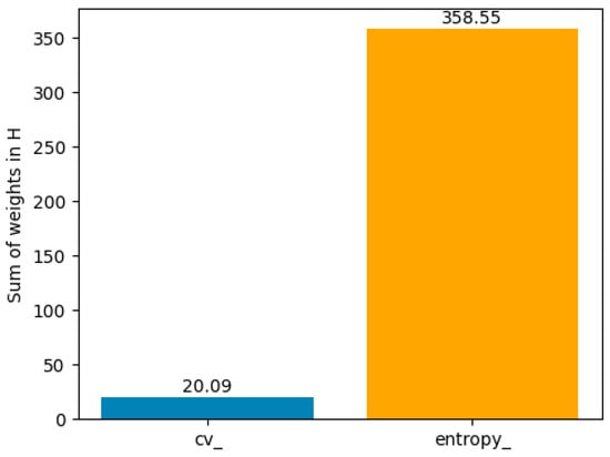
Figure 12.
Profile 1—distribution of weights (CV vs. entropy).
Profile 1 is characterized by high variability (CV = 403.99) and lower entropy (224.41), while Profile 2 shows low variability (CV = 20.09) and higher entropy (358.55).
These numerical summaries reinforce the contrast between profiles and provide a clearer quantitative interpretation.
Table 10 presents the functional characterization for February 2017.
Table 10.
Functional characterization of latent profiles (February 2017).
In terms of CV, the profiles are sharply separated: Profile 0 shows a high average CV (0.74, SD = 0.13, IQR = 0.12), while Profile 1 shows a low average CV (0.34, SD = 0.11, IQR = 0.15). Even when considering dispersion, the ranges do not overlap, confirming that variability in consumption is a strong differentiating factor. This reflects heterogeneity in Profile 0 and relative homogeneity in Profile 1, with no ambiguity between them.
Entropy, however, reveals a subtler picture. Profile 0 exhibits lower average entropy (0.84, SD = 0.06, IQR = 0.05), indicating heterogeneous and less structured behaviors. Profile 1 shows higher average entropy (0.92, SD = 0.02, IQR = 0.02), reflecting homogeneous and highly structured behaviors. Although the averages distinguish the profiles, dispersion measures reveal partial overlap: adding one SD to Profile 0 yields 0.91, while subtracting one SD from Profile 1 gives 0.90.
This overlap suggests that a subset of flexible users can display structural behaviors comparable to stable users.
Thus, CV separates the profiles sharply, while entropy highlights heterogeneity and a diffuse boundary between flexibility and stability.
Profile 0, though minoritarian, represents highly flexible users, while Profile 1 corresponds to stable, less adaptable users.
3.2.4. Clustering on Latent Profiles
K-Means applied to the latent representation (W) produced four functional clusters (A, B, C, D). Cosine similarity analysis confirmed that these clusters remain structurally stable across months. To illustrate their internal characterization, Table 11 presents the results for January 2017, showing average activation of latent profiles, coefficient of variation (CV), and entropy (H) for each cluster.
Table 11.
Structural characterization of latent functions (January 2017).
Cluster A exhibits low variability and high entropy, reflecting stable and distributed consumption patterns. Cluster B shows moderate variability and intermediate entropy, associated with heterogeneous behaviors. Cluster C represents an intermediate group balancing stability and variability. Cluster D concentrates the most variable users, with high CV and lower entropy, indicating greater flexibility potential.
These results demonstrate that the combination of NMF and K-Means yields a robust segmentation of users, distinguishing groups with different degrees of stability and flexibility. This differentiation provides a technical basis for designing demand response strategies: highly variable clusters (B and D) can be prioritized for dynamic programs, while stable clusters (A and C) are more suitable for efficiency measures or indirect control schemes.
3.3. Hourly Characterization and Economic Potential of Energy Flexibility
Beyond the identification of latent profiles and functional clusters, it is necessary to evaluate how flexibility manifests in the temporal distribution of electricity consumption. This section characterizes the average hourly load curves for each latent function (A–D) and estimates the economic and reliability impacts associated with their flexibility. The objective is not to redefine the structural metrics already presented (CV and entropy), but to complement them with operational evidence that highlights the potential benefits of load redistribution.
3.3.1. Hourly Consumption Patterns
Figure 13, Figure 14, Figure 15 and Figure 16 show the average hourly curves by day of the week for each latent function. Function A concentrates demand in the evening (19 h–22 h), reflecting rigid routines and low flexibility. Function B exhibits a bimodal structure (morning and evening), suggesting moderate flexibility. Function C shows a dominant evening peak with minor morning activity, representing an intermediate group. Function D displays dispersed peaks across the day, indicating the highest flexibility potential. These patterns confirm the structural interpretation derived from CV and entropy, while providing a clearer operational view of consumption behaviors.
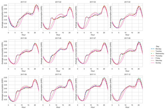
Figure 13.
Average hourly curve—Function A.
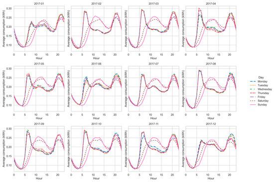
Figure 14.
Average hourly curve—Function B.
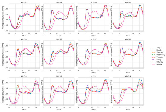
Figure 15.
Average hourly curve—Function C.
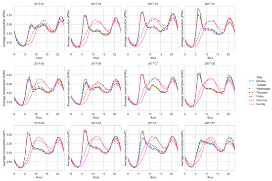
Figure 16.
Average hourly curve—Function D.
Figure 17 illustrates representative hourly consumption curves with variance bands for November 2017. Each latent function is shown with its average profile and the corresponding dispersion across users. This visualization complements the structural interpretation by highlighting the variability within each group, offering a clearer operational view of flexibility potential.
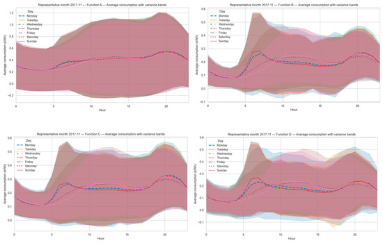
Figure 17.
Representative hourly consumption curves with variance bands for November 2017. Each subplot corresponds to one latent function (A–D).
3.3.2. Economic Estimation of Flexibility
Applying the simulation framework described in Section 2 was applied to Functions B and D, identified as the most flexible groups. Redistribution scenarios of 5%, 10% and 20% of peak-hour load were evaluated.
Figure 18, Figure 19, Figure 20, Figure 21, Figure 22 and Figure 23 illustrate the redistribution effect on hourly load curves. In all cases, energy is shifted from peak hours (≥90% of daily maximum) to valley hours (≤70% of daily maximum), maintaining constant total daily consumption. The difference between base and flexible scenarios is especially evident on weekends, where a larger share of load can be shifted.
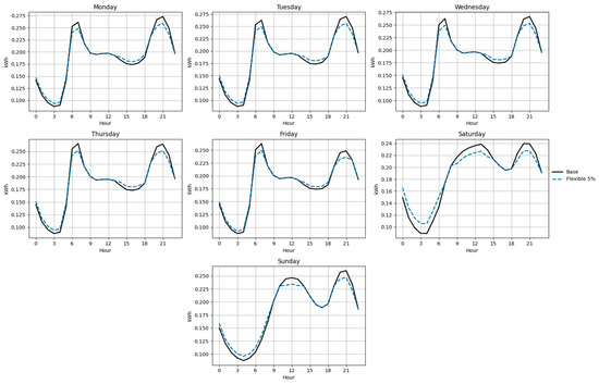
Figure 18.
Base and flexible curves for Function B (5%).
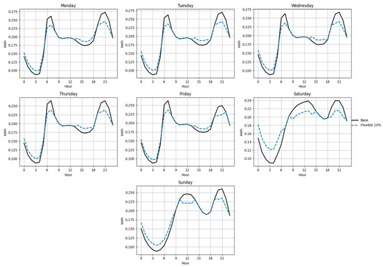
Figure 19.
Base and flexible curves for Function B (10%).
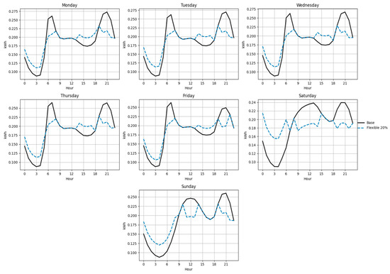
Figure 20.
Base and flexible curves for Function B (20%).
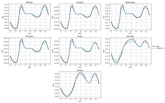
Figure 21.
Base and flexible curves for Function D (5%).
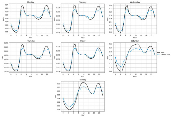
Figure 22.
Base and flexible curves for Function D (10%).
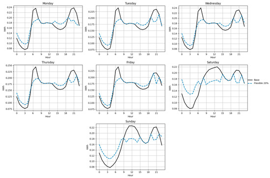
Figure 23.
Base and flexible curves for Function D (20%).
Table 12 summarizes the annual savings obtained under each redistribution scenario. The results show that, although individual savings remain modest compared to a typical monthly bill of approximately 100,000 COP (≈27 USD), the aggregated impact across the user population is significant. Function B consistently exhibits higher savings than Function D, reflecting its structural flexibility and greater potential for economic optimization.
Table 12.
Annual economic savings under simulated tariff (2017, expressed in USD).
3.4. Reliability Estimation of Flexibility
Beyond the individual economic benefits, flexibility also contributes to system reliability. Applying the methodological framework described in Section 2.6, redistribution scenarios of 5%, 10% and 20% of peak-hour load were simulated for flexible functions (B and D), while rigid functions (A and C) remained unchanged. The equivalent sector of 1000 users and the system capacity limit of 0.36 MW provided the basis for quantifying improvements in reliability indices.
Table 13 summarizes the annual reliability indicators (SAIDI, SAIFI and ENS) under each redistribution scenario. Even moderate flexibility (5%) yields significant improvements, while 10% further reduces interruptions and 20% eliminates overloads completely. In addition to improved service continuity, the reduction in ENS translates into additional revenues for the operator, complementing the individual savings of users.
Table 13.
Annual reliability results (SAIDI, SAIFI, and ENS) under adaptive redistribution scenarios.
Figure 24, Figure 25 and Figure 26 illustrate the sectoral curves for March 2017, showing how redistribution reduces critical peaks and shifts load into safe hours. In each case, SAIDI and SAIFI values are annotated before and after redistribution, evidencing the improvement in reliability.
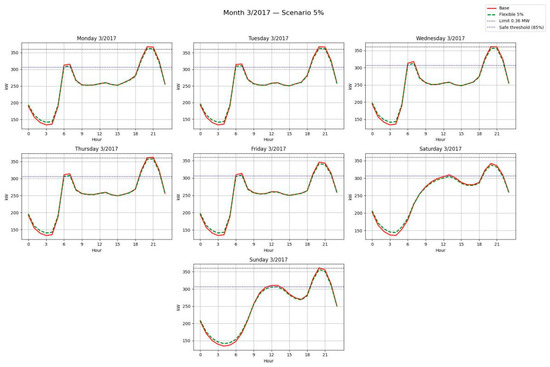
Figure 24.
Average sectoral curves by day of the week—Base vs. Flexible scenario (5%).
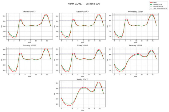
Figure 25.
Average sectoral curves by day of the week—Base vs. Flexible scenario (10%).
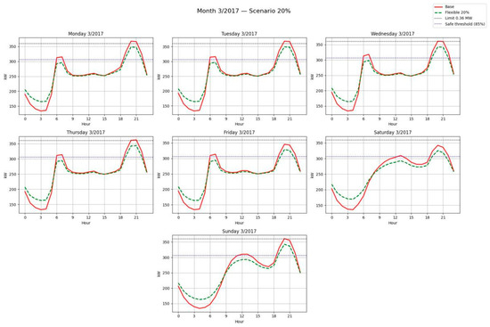
Figure 26.
Average sectoral curves by day of the week—Base vs. Flexible scenario (20%).
Overall, these results confirm that energy flexibility not only generates economic benefits (Section 3.3), but also contributes significantly to service quality by reducing both the duration and frequency of interruptions. This dual impact reinforces the strategic value of flexibility as a demand-side resource, simultaneously improving system reliability and optimizing economic efficiency.
4. Discussion
The results obtained in Section 3 provide a comprehensive view of how demand-side flexibility manifests in residential electricity consumption. From preliminary statistical analyses (CV and entropy), through clustering and latent profile identification, to the quantification of economic and reliability impacts, the findings consistently support the working hypothesis that flexibility is a valuable operational resource.
In relation to previous studies, the observed heterogeneity across day types and user groups aligns with evidence that variability in routines is a key determinant of flexibility potential. The clustering outcomes confirm that segmentation based on structural metrics can distinguish groups with different adaptability levels, a result consistent with literature on demand response targeting. Moreover, the economic simulations demonstrate that while individual savings are modest, aggregated impacts are significant, reinforcing the notion that collective participation is essential for program viability. This echoes findings from international experiences where household-level incentives are small but system-level benefits are substantial.
The reliability improvements quantified through SAIDI, SAIFI, and ENS further high-light the operational value of flexibility. Even moderate redistribution (5–10%) yields notable reductions in interruptions, while 20% eliminates overloads entirely. These results are consistent with prior work emphasizing the role of demand response in enhancing continuity of supply and mitigating stress on distribution networks. Importantly, the dual impact, economic and reliability, underscores that flexibility should be considered not only as a market mechanism but also as a tool for improving equity in service provision.
An additional consideration relates to the assumption of a fixed tariff structure. Al-though the dataset covers multiple municipalities across Bogotá D.C., Cundinamarca, and Tolima, the simulations adopted official values for Bogotá in 2017, used as a representative benchmark due to their availability and regulatory relevance. Tariff levels are subject to regulatory changes, fuel price dynamics, and exchange rate fluctuations. Sensitivity analyses indicate that moderate variations (±10% in peak and valley tariffs) do not alter the qualitative conclusions: Function B consistently yields higher savings than Function D, and aggregated impacts remain significant. However, the magnitude of individual savings scales proportionally with tariff differentials, suggesting that stronger peak penalties or valley incentives could enhance the economic attractiveness of flexibility programs. This reinforces the robustness of the findings while highlighting the importance of regulatory design in shaping demand response outcomes.
A methodological limitation relates to data granularity. The analyses were conducted using hourly records, which provide a robust basis for identifying structural patterns and long-term flexibility potential. However, sub-hourly data (e.g., 15 min or minute-level intervals) could capture short-term fluctuations, appliance-level dynamics, and rapid load-shifting opportunities that are not visible in hourly aggregates. Consequently, the results may underestimate the operational flexibility available at finer temporal resolutions. Future work should incorporate sub-hourly datasets to validate the robustness of the findings and to explore the additional value of high-frequency demand response actions.
A further limitation concerns the location-specific nature of the results. The analyses were conducted using consumption data from Bogotá, under Colombian tariff structures and regulatory conditions. While the methodological framework is transferable, the quantitative outcomes reflect local cultural routines, appliance penetration, and institutional arrangements. Generalization to other regions therefore requires caution, as differences in tariff design, climatic conditions, and user behavior may alter both the magnitude and distribution of flexibility potential. Future studies should replicate the approach in diverse contexts to validate its applicability and to identify region-specific drivers of demand-side flexibility.
In the broader context, these findings contribute to ongoing discussions on the modernization of distribution systems and the energy transition. Flexibility emerges as a demand-side resource that complements supply-side investments, enabling more efficient use of existing infrastructure. Future research should explore scalability under different penetration levels of flexible technologies, integration with distributed energy resources (DERs), and behavioral aspects of user adoption. Such directions will help assess the long-term sustainability of flexibility programs and their role in achieving decarbonization goals.
Overall, the study confirms that demand-side flexibility is a viable pathway to simultaneously improve economic efficiency and system reliability. By situating these results within the broader literature, the contribution extends beyond local case studies, offering insights relevant to international debates on energy transition and demand response strategies.
5. Conclusions
This study demonstrates that energy flexibility is a structural property of residential consumption, defined not by absolute demand levels but by the capacity to redistribute load over time without compromising user functionality. Statistical metrics such as the coefficient of variation and normalized entropy revealed critical behavioral windows: rigid stability in early mornings (5–7 h) and high heterogeneity in evening hours (21–23 h). Weekly and seasonal analyses confirmed that flexibility is not uniformly distributed, but concentrated in transitional days and months, reflecting social and cultural dynamics embedded in energy data.
Dimensionality reduction through Non-Negative Matrix Factorization (NMF) proved essential to uncover coherent latent structures in consumption. Direct clustering on high-dimensional matrices failed to differentiate users consistently, whereas NMF extracted robust and temporally stable profiles. Subsequent clustering identified four functional trajectories (A–D), with B and D exhibiting the highest flexibility potential. These groups, characterized by dispersed or bimodal load patterns, are capable of shifting demand from critical to safe hours, thereby reducing system stress and enhancing operational stability.
Economic simulations showed that individual savings remain modest, yet aggregated impacts are significant. Flexible trajectories achieved annual savings between 0.39 and 2.15 USD per user, translating into 4270–17,030 USD when scaled to the population. Reliability simulations confirmed that redistributing 5–20% of peak load reduces SAIDI and SAIFI substantially and recovers up to 114 kWh of unsupplied energy. This dual impact—economic and reliability—consolidates flexibility as a strategic demand-side resource.
Finally, the comparative evaluation of predictive models (ARIMA vs. ARX) high-lighted that no single approach guarantees superior performance across all trajectories. Model selection must adapt to the structural nature of each profile. Overall, the methodology applied provides a reproducible framework for identifying flexibility potential, quantifying its economic and operational value, and supporting adaptive demand management strategies in the context of energy transition.
Author Contributions
Conceptualization, J.R.-G.; methodology, J.R.-G.; software, J.O.-L.; validation, J.O.-L. and J.R.-G.; formal analysis, J.O.-L.; investigation, J.O.-L.; resources, J.R.-G.; data curation, J.O.-L.; writing—original draft preparation, J.O.-L.; writing—review and editing, J.O.-L. and J.R.-G.; visualization, J.O.-L.; supervision, J.R.-G.; project administration, J.R.-G. All authors have read and agreed to the published version of the manuscript.
Funding
This research was supported by Electrical Machines and Drives (EM&D) from Universidad Nacional de Colombia, Energy Solutions Cooperation Network for Communities, code: 59384.
Data Availability Statement
The data presented in this study are not publicly available due to confidentiality agreements with the industrial facility where the measurements were obtained.
Conflicts of Interest
The authors declare no conflicts of interest.
Abbreviations
The following abbreviations are used in this manuscript:
| AMI | Advanced Metering Infrastructure |
| CV | Coefficient of Variation |
| ENS | Energy Not Supplied (Unsupplied Energy) |
| NMF | Non-Negative Matrix Factorization |
| SAIDI | System Average Interruption Duration Index |
| SAIFI | System Average Interruption Frequency Index |
| TRM | Tasa Representativa del Mercado (Exchange Rate) |
| USD | United States Dollar |
| σ | Standard deviation |
| µ | Mean (average) |
| IQR | Interquartile Range (Q75 − Q25) |
| n | Sample size (number of observations) |
| pi/pj | Probability of event i or j |
| H | Shannon entropy |
| Hnorm | Normalized entropy |
| k | Number of bins/events |
| V | Original non-negative data matrix |
| W | User latent representation matrix |
| H(profiles) | Latent profile matrix (weights of variables) |
| cos(A, B) | Cosine similarity between vectors A and B |
References
- Bustos-Brinez, O.A.; Zambrano-Pinto, A.; Rosero Garcia, J. Application of data analysis techniques for characterization and estimation in electrical substations. Front. Energy Res. 2024, 12, 1372347. [Google Scholar] [CrossRef]
- Wang, Y.; Chen, Q.; Hong, T.; Kang, C. Review of Smart Meter Data Analytics: Applications, Methodologies, and Challenges. IEEE Trans. Smart Grid 2019, 10, 3125–3148. [Google Scholar] [CrossRef]
- Ahmad, T.; Zhang, D.; Huang, C.; Zhang, H.; Dai, N.; Song, Y.; Chen, H. Artificial intelligence in sustainable energy industry: Status Quo, challenges and opportunities. J. Clean. Prod. 2021, 289, 125834. [Google Scholar] [CrossRef]
- Hossain, E.; Khan, I.; Un-Noor, F.; Sikander, S.S.; Sunny, M.S.H. Application of Big Data and Machine Learning in Smart Grid, and Associated Security Concerns: A Review. IEEE Access 2019, 7, 13960–13988. [Google Scholar] [CrossRef]
- Ullah, Z.; Al-Turjman, F.; Mostarda, L.; Gagliardi, R. Applications of Artificial Intelligence and Machine learning in smart cities. Comput. Commun. 2020, 154, 313–323. [Google Scholar] [CrossRef]
- Grolinger, K.; L’Heureux, A.; Capretz, M.A.; Seewald, L. Energy Forecasting for Event Venues: Big Data and Prediction Accuracy. Energy Build. 2016, 112, 222–233. [Google Scholar] [CrossRef]
- Hu, J.; Vasilakos, A.V. Energy Big Data Analytics and Security: Challenges and Opportunities. IEEE Trans. Smart Grid 2016, 7, 2423–2436. [Google Scholar] [CrossRef]
- Toledo-Cortés, S.; Lara, J.S.; Zambrano, A.; Osorio, F.A.G.; Garcia, J.R. Characterization of electricity demand based on energy consumption data from Colombia. Int. J. Electr. Comput. Eng. 2023, 13, 4798–4809. [Google Scholar] [CrossRef]
- Kwac, J.; Flora, J.; Rajagopal, R. Household Energy Consumption Segmentation Using Hourly Data. IEEE Trans. Smart Grid 2014, 5, 420–430. [Google Scholar] [CrossRef]
- Maamar, A.; Benahmed, K. A Hybrid Model for Anomalies Detection in AMI System Combining K-means Clustering and Deep Neural Network. Comput. Mater. Continua 2019, 60, 15–39. [Google Scholar] [CrossRef]
- Estrada, J.H.; Cano-Plata, E.A.; Younes-Velosa, C.; Cortés, C.L. Entropy and coefficient of variation (CV) as tools for assessing power quality. Ing. Investig. 2011, 31, 45–50. [Google Scholar] [CrossRef]
- Wang, Y.; Chen, Q.; Kang, C.; Xia, Q. Clustering of Electricity Consumption Behavior Dynamics Toward Big Data Applications. IEEE Trans. Smart Grid 2016, 7, 2437–2447. [Google Scholar] [CrossRef]
- Zapata Flórez, P.A.; Castro Zuluaga, C.A. CARACTERIZACIÓN DE DEMANDA PARA AJUSTAR LA CONFIGURACIÓN DE UN MÉTODO DE PRONÓSTICOS EN LA CADENA DE SUMINISTROS. Master’s Thesis, Universidad EAFIT, Medellín, Colombia, 2020. Available online: https://repository.eafit.edu.co/server/api/core/bitstreams/803d2fe0-9ba6-469b-9375-536cb00fdb4d/content (accessed on 20 September 2025).
- Everitt, B. The Cambridge Dictionary of Statistics; Cambridge University Press: Cambridge, UK, 2010. [Google Scholar]
- Freedman, D.; Diaconis, P. On the histogram as a density estimator: L2 theory. Z. Wahrscheinlichkeitstheorie Verwandte Geb. 1981, 57, 453–476. [Google Scholar] [CrossRef]
- Scott, D.W. Scott’s rule. WIREs Comput. Stat. 2010, 2, 497–502. [Google Scholar] [CrossRef]
- Siano, P. Demand response and smart grids—A survey. Renew. Sustain. Energy Rev. 2014, 30, 461–478. [Google Scholar] [CrossRef]
- Palensky, P.; Dietrich, D. Demand Side Management: Demand Response, Intelligent Energy Systems, and Smart Loads. IEEE Trans. Ind. Inform. 2011, 7, 381–388. [Google Scholar] [CrossRef]
- Afzalan, M.; Jazizadeh, F. Residential loads flexibility potential for demand response using energy consumption patterns and user segments. Appl. Energy 2019, 254, 113693. [Google Scholar] [CrossRef]
- Si, C.; Xu, S.; Wan, C.; Chen, D.; Cui, W.; Zhao, J. Electric Load Clustering in Smart Grid: Methodologies, Applications, and Future Trends. J. Modern Power Syst. Clean Energy 2021, 9, 237–252. [Google Scholar] [CrossRef]
- McLoughlin, F.; Duffy, A.; Conlon, M. A clustering approach to domestic electricity load profile characterisation using smart metering data. Appl. Energy 2015, 141, 190–199. [Google Scholar] [CrossRef]
- Xu, W.; Liu, X.; Gong, Y. Document clustering based on non-negative matrix factorization. In Proceedings of the 26th Annual International ACM SIGIR Conference on Research and Development in Information Retrieval, Toronto, Canada, 28 July–1 August 2003; ACM: New York, NY, USA, 2003; pp. 267–273. [Google Scholar] [CrossRef]
- Paatero, P.; Tapper, U. Positive matrix factorization: A non-negative factor model with optimal utilization of error estimates of data values. Environmetrics 1994, 5, 111–126. [Google Scholar] [CrossRef]
- Iglesias, F.; Kastner, W. Analysis of Similarity Measures in Times Series Clustering for the Discovery of Building Energy Patterns. Energies 2013, 6, 579–597. [Google Scholar] [CrossRef]
- Hafeez, G.; Alimgeer, K.S.; Wadud, Z.; Khan, I.; Usman, M.; Qazi, A.B.; Khan, F.A. An Innovative Optimization Strategy for Efficient Energy Management with Day-Ahead Demand Response Signal and Energy Consumption Forecasting in Smart Grid Using Artificial Neural Network. IEEE Access 2020, 8, 84415–84433. [Google Scholar] [CrossRef]
- Bustos-Brinez, O.A.; Duarte, J.E.; Zambrano-Pinto, A.; González, F.A.; Rosero-Garcia, J. A Method for the Characterization of the Energy Demand Aggregate Based on Electricity Data Provided by AMI Systems and Metering in Substations. Energies 2024, 17, 87. [Google Scholar] [CrossRef]
- Wang, Y.; Chen, Q.; Kang, C.; Zhang, M.; Wang, K.; Zhao, Y. Load profiling and its application to demand response: A review. Tsinghua Sci. Technol. 2015, 20, 117–129. [Google Scholar] [CrossRef]
- Shannon, C.E. A mathematical theory of communication. Bell Syst. Tech. J. 1948, 27, 379–423. [Google Scholar] [CrossRef]
- Superintendence of Public Utilities. Electricity Tariff Bulletin-First Quarter 2017. 2017. Available online: https://www.superservicios.gov.co/sites/default/files/inline-files/20170507_boletin_tarifario_i_trimestre_2017_08052017_final_1.pdf (accessed on 15 November 2025).
- Banco de la República de Colombia. Tasa de Cambio-TRM. Exchange Rate: 1 USD = 3,700.05 COP. 2026. Available online: https://www.banrep.gov.co/es/glosario/tasa-cambio-trm (accessed on 20 January 2026).
- Haben, S.; Singleton, C.; Grindrod, P. Analysis and Clustering of Residential Customers Energy Behavioral Demand Using Smart Meter Data. IEEE Trans. Smart Grid 2016, 7, 136–144. [Google Scholar] [CrossRef]


Disclaimer/Publisher’s Note: The statements, opinions and data contained in all publications are solely those of the individual author(s) and contributor(s) and not of MDPI and/or the editor(s). MDPI and/or the editor(s) disclaim responsibility for any injury to people or property resulting from any ideas, methods, instructions or products referred to in the content. |
© 2026 by the authors. Licensee MDPI, Basel, Switzerland. This article is an open access article distributed under the terms and conditions of the Creative Commons Attribution (CC BY) license.