Fracture Conductivity and Its Effects on Production Estimation in Shale

Abstract

This study investigates the impact of fracture conductivity on hydraulically fractured wells in the Eagle Ford Shale using commercial simulation software. Motivated by recent findings on conductivity degradation and the proven reliability of sensitivity analyses in shale reservoirs, a 17-stage horizontal well was modeled to evaluate productivity optimization. The methodology involved holding fracture fluid volume constant while analyzing conductivity variations across both single-fracture and full-well models. Production simulations were validated against real-time field data. Results indicate that the simulation models accurately represent the reservoir, with single-fracture scenarios yielding similar cumulative production and full-well models showing only minor deviations. Ultimately, the observed differences do not justify a significant deviation from current completion techniques under the modeling assumptions considered, as infinite-acting flow remains the dominant regime due to the reservoir’s low permeability.

1. Introduction

1.1. Background

Conventional resources have historically played a major role in the United States oil and gas industry. However, the gradual decline of these conventional plays has driven the development of alternative production strategies. This shift led to the exploitation of unconventional reservoirs and the widespread adoption of horizontal drilling and hydraulic fracturing technologies. Optimizing the economic efficiency of horizontal well drilling has therefore become a central focus in unconventional reservoir development. As these technologies matured, drilling and completion operations became increasingly standardized, enabling rapid well deployment. Nevertheless, determining the optimal hydraulic fracture geometry remains a complex challenge and continues to require robust numerical simulation approaches to improve operational efficiency [1].

In addition, production-stage processes such as pressure depletion, fluid–rock interactions, and near-wellbore impairment mechanisms can significantly influence effective flow capacity within the reservoir. These processes highlight the need for comprehensive numerical simulation frameworks capable of capturing both fracture behavior and reservoir performance evolution over time [2,3].

The primary objective of this study is to improve the understanding of hydraulic fracturing performance through numerical simulation. Specifically, the impact of fractured conductivity on production behavior in the Eagle Ford Shale is investigated. A reservoir simulation model is developed to evaluate the effects of fracture conductivity during production using a horizontal well with 17 fracture stages. Fracture conductivity is varied by adjusting fracture width and height, and the resulting production response is analyzed under depletion conditions. The outcomes of this study provide improved insight into fracture conductivity and its implications for well productivity and economic performance.

1.2. Geomechanics

There are three principal stresses: the maximum horizontal stress, minimum horizontal stress, and vertical stress. These three stresses play a large role in determining the effectiveness of horizontal well hydraulic fracturing. Fractures are drilled perpendicular to the maximum horizontal stress and propped open with pressure and sand. Usually, the fracture opens to both sides of the wellbore and creates a bi-wing fracture. In depleted reservoirs, this is not always the case; therefore, wells are spaced out properly when a field is initially being developed.

One of the most noticeable changes during depletion is the decrease in pore pressure from production, and because of that, the minimum horizontal stress decreases as well. Depletion can also cause porosity loss, which in turn affects permeability, and it can sometimes rotate the principal stresses. It is established that rock deformation occurs simultaneously with gas flow during production, impacting reservoir flow behaviors [4]. As the fluid leaves the reservoir, the sand will begin to compact, and this will reduce the porosity. Research indicates that as effective stress increases during drawdown, fracture permeability decreases significantly due to stress sensitivity, directly impacting the Estimated Ultimate Recovery (EUR) [5]. Furthermore, dynamic conductivity models show that fractures gradually close as hydrocarbons are extracted, creating distinct flow regimes that must be accounted for in simulation [6]. If the reservoir is weakly cemented, then compaction can greatly affect the fluid flow.

1.3. Fracture Geometry

The geometry of a well’s fractures can significantly affect the production performance of a horizontal well. Fracture simulations must operate on simplifying assumptions to develop a manageable model. Unlike the complexities of reality, these models often rely on a few key assumptions: that only one linear crack exists in the reservoir, that the entire length of this fracture actively contributes to fluid flow, and that the fracture behaves as if it were infinite-acting. While these assumptions introduce some error, they still enable the development of a sound and effective production model.

The primary objective of hydraulic fracturing is to increase the total surface area through which the well can contact the reservoir rock. Increasing the fracture length is widely considered one of the most effective ways to achieve optimal contact in a horizontal well configuration. Generally, lower reservoir permeability requires longer fracture lengths to optimize project economics. The overall fracture geometry is also critically influenced by both fracture width and the spacing between individual fracture stages.

1.4. Fracture Conductivity

Understanding how fracture conductivity is measured in the field versus in the laboratory can help engineers create more effective fractures and elucidate the mechanisms that govern fracture conductivity.

Field-measured fracture conductivity is often significantly lower than the conductivity measured in a controlled laboratory setting. Several key factors contribute to this discrepancy:

(1)

Non-Darcy Flow and Multiphase Flow effects: These complex fluid dynamics are often oversimplified or absent in lab tests but present significant resistance in the field.

(2)

Proppant Loading: Real-world distribution and concentration of proppant (the material used to keep fractures open) often differ from ideal lab conditions.

(3)

Embedment and Spalling: The crushing of formation rock (embedment) or the failure of the rock surface (spalling) under closure stress can reduce the effective flow path width in situ [7].

(4)

Temperature Effects: The high downhole temperatures and pressures encountered in actual reservoirs affect fluid viscosity and rock/proppant mechanics differently than ambient lab conditions.

1.5. Theory

Engineers utilize reservoir simulation to model reservoir behavior and forecast future performance. This process requires inputting specific reservoir properties, including permeability, porosity, net pay thickness, water saturation, and various fluid characteristics, into a modeling program. This study employs the Eclipse simulator to construct an artificial reservoir model, using accurate input data to ensure reliable outcomes when evaluating different production strategies. While various simulation types exist, they are typically executed using either analytical or explicit numerical methods.

1.6. Comparison of Analytical and Numerical Modeling

Sadrpanah et al. [8] conducted a comparative analysis of analytical and numerical modeling techniques. The study demonstrated that analytical simulation often fails to account for well geometry or the heterogeneous geology of the different sands a well might connect. Instead, it relies on an equivalent wellbore radius to represent the created fracture and computes the productivity index (PI) to account for this larger radius.

In contrast, numerical simulation employs the transmissibility of connecting grid blocks to model conductivity. Transmissibility is obtained as a harmonic average by defining a single permeability and porosity for each grid block. This approach allows for detailed rock properties and multiple layers to be incorporated into the simulation.

1.7. Advantages of Numerical Simulation

Numerical simulations are superior to analytical models for several critical parameters, particularly when addressing complex geomechanical and fluid-dynamics problems.

(1)

Multiphase Flow: Numerical models can accurately predict the well’s productivity index by accounting for multiphase flow after history matching.

(2)

Geomechanical and Contact Analysis: Numerical methods, such as the finite element code in ANSYS Mechanical APDL 19.2 (2018 R2), can simulate complex behaviors like the formation/proppant contact-impact behavior in fracture surfaces [9]. These codes can introduce material properties of proppants and formation characteristics to calculate deformation and total penetration depth [9].

(3)

Fluid Flowback and Injection: Numerical simulation is also effective for evaluating flowback efficiency under varying conditions. For example, simulations can model proppant transport in complex fracture geometries and evaluate the impact of different injection rates or fluid types (e.g., CO₂ versus water-based) on recovery efficiency [10].

(4)

Water or Gas Coning: Because analytical simulation does not account for the geology surrounding the well, numerical simulation is more effective for modeling coning effects, which can significantly impact production. This is equally true for vertical fractures intersecting multiple formations.

(5)

Non-Darcy Flow and Geometry: Numerical modeling accounts for non-Darcy flow effects and precise reservoir geometry and well location, facilitating better economic decisions regarding the well’s future.

1.8. Local Grid Refinement (LGR)

One of the most important techniques used in reservoir simulation is Local Grid Refinement (LGR). LGR is a simulation method that creates a coarse grid around the near-wellbore area to model early transient pressure for a single well. While this technique is not necessary for a full-field model, it is valuable for localized analysis. When the LGR method is utilized, block sizes are decreased, and the oil production plateau is often shortened due to the modeling of higher, more realistic flow rates near the wellbore.

Recent studies have increasingly applied data-driven and machine learning (ML) approaches to estimate fracture conductivity in shale reservoirs based on geological properties, proppant characteristics, and completion parameters. For example, Meyer [11] developed a machine-learning-based framework to predict fracture conductivity under varying reservoir and treatment conditions, demonstrating the potential of data-driven methods for conductivity estimation. While these approaches focus on predicting fracture conductivity values, fewer studies have examined how different spatial distributions of fracture conductivity influence production behavior once conductivity is specified. In this context, numerical reservoir simulation provides a complementary framework by linking fracture conductivity distributions to well productivity and cumulative production response.

2. Methodology

2.1. Reservoir and Simulation Model Setup

In this study, a previously generated model was used from “Fracture Geometry Modeling and Its Effects on Production Estimation in Shale”, Luong. The base numerical model was originally developed to represent a hydraulically fractured horizontal well in the Eagle Ford Shale and was validated by matching productivity index and cumulative production trends reported for comparable field-scale wells. Key assumptions carried forward into the present study include homogeneous reservoir properties within each grid block, single planar bi-wing fractures per stage, constant fracture height, and isothermal flow conditions. These assumptions are consistent with established shale reservoir simulation practices and are appropriate for evaluating relative fracture conductivity effects rather than absolute production forecasting.

The grid of the blocks was exactly the same, with a total grid size of 1600 ft × 5000 ft × 300 ft in the X, Y, and Z directions. This design of grid blocks gives a shape of a rectangular prism. In the data file, all the properties such as oil PVT, lithology are similar to the Eagle Ford Shale formation.

Actual completion data are used in the simulations. This gives an accurate representation of a real-world well. The horizontal well is drilled through the middle of the reservoir at 10,892 feet. There are 17 fracture stages in the well. The total amount of fracture fluid used is 2,736,820 gallons containing Linear Gel and X-Link Gel. Ideally, this would give each fracture stage 160,989 gallons of fluid for the frac. This information can now act as guidelines for the simulations, and different scenarios can be created.

Several different fracture conductivity models were set up using Eclipse 100. The models tested different fracture conductivity placements in a fracture. The simulations were then run for 30 days to compare to the actual production. The results were then considered to see how different fracture conductivities affect the simulation results. Then, the simulations were run again at 1440 days for all the models. The results were observed.

2.2. Reservoir Properties and Grid Parameters

Data was collected and analyzed to select the optimum properties for the Eagle Ford Shale reservoir. The geometry of the well is designed to be similar to a typical well that can be found in the Eagle Ford Shale. The data seen below represents the data that were selected for the upcoming simulation models.

The data (as shown in Table 1) creates a grid that is 40 × 100 × 20. It also gives the conditions for some of the basic reservoir qualities such as permeability, formation thickness, porosity, API gravity, and the initial reservoir pressure.

Table 1. Reservoir data for simulation.

Variable	Value	Unit
Thickness	300	Feet
Permeability, X	8.5 × 106	mD
Permeability, Y	8.5 × 106	mD
Permeability, Z	5 × 109	mD
Porosity	8	%
Length, X	1600	Feet
Length, Y	5000	Feet
Length, Z	300	Feet
Number of Blocks, X	40
Number of Blocks, Y	100
Number of Blocks, Z	20
Initial Water Saturation	20	%
Initial Gas Saturation	0	%
Wellbore Diameter	0.25	%
Tops	10,742	Feet
API Gravity	42
Initial Pressure	6263	psi

2.3. Completion Design and Fracture Properties

Table 2 shows the actual completion data for a well in the Eagle Ford Shale. Fracture properties are based on this information for the simulations.

Table 2. Actual completion data.

Variable	Value	Unit
State	Texas
County	Atascosa
True Vertical Depth	10,742	Feet
Completion Length	4280	Feet
Number of Frac Stages	17
Acid	74,710	Gallons
Slick Water	0	Gallons
Linear Gel	56,040	Gallons
X-Link Gel	2,099,070	Gallons
Fracture Width	0.02	Feet
Average Conductivity	1529	mD·ft

When modeling a hydraulic fracture, it is important to remember that fracture qualities are different than reservoir qualities, especially in shale formations. The largest difference can be seen in the difference in permeability. The reservoir permeability is 8.5 × 10⁻⁶ mD (8.5 nano-darcies), while the fracture permeability and the fracture permeability re calculated from the completion data are 76,450 milli-darcies. This is a large difference that plays a huge role in modeling hydraulic fractures.

2.4. Fracture Modeling Approach

In the simulation, the wellbore diameter is assumed to be 0.25 feet. This is an appropriate assumption, but it creates a problem for modeling purposes. Eclipse will not perform a simulation if the grid block is smaller than the wellbore. If a true fracture were to be modeled, it would be 0.01 feet to 0.1 feet in width, so it is impossible to actually create a grid block small enough for a realistic fracture. Therefore, it is necessary to devise a way to model an appropriate fracture. The technique for adjusting the grid can be seen below in Equations (1) and (2).

$$F_{CD}={\displaystyle \frac{K_f\times W_f}{{K\times X}_f}}$$

(1)

$$k_{fe}={\displaystyle \frac{K_f{W}_f}{W_e}}={\displaystyle \frac{F_{CD}}{W_e}}$$

(2)

where $K_f$ is the fracture permeability, $W_f$ is the fracture width, and $X_f$ is the fracture length; K is the reservoir permeability; $K_{fe}$ is the equivalent fracture permeability; $W_e$ is the equivalent fracture width; and $F_{CD}$ is the fracture conductivity.

Using these two formulas, the fracture width can now be enlarged to 2 ft. A two-foot fracture is not realistic in a real formation, so the equivalent fracture permeability is then adjusted. Now, in the model, there is a much wider fracture, but it has a lower permeability. This is a key assumption in the model and should give close-to-accurate results.

The average conductivity of 1529 mD is taken into account in the scenarios so that a comparison can be viewed. The average conductivity acts as another restraint that is very similar to the fracture width. If the average conductivity is not honored, the model results could be skewed to show an unrealistic result in the simulation models.

Fracture conductivity in this study is represented using an equivalent fracture modeling approach, in which fracture width is increased while fracture permeability is adjusted to preserve the target conductivity. This approach is widely adopted in numerical reservoir simulation due to its numerical stability and compatibility with finite-difference grid formulations. In Eclipse, fracture flow is modeled through enhanced transmissibility between fracture grid cells and adjacent reservoir cells, enabling representation of fracture-dominated flow within the standard grid framework.

It is acknowledged that this equivalent fracture representation does not explicitly capture near-wellbore pressure gradients, non-Darcy flow effects at high velocities, or detailed proppant transport and embedment mechanisms. In addition, fracture conductivity degradation with time was not explicitly modeled in this study. Instead, fracture conductivity was assumed to be constant to isolate the impact of spatial conductivity distribution on production behavior. These limitations are acceptable within the scope of this work, which focuses on comparative analysis of conductivity distribution effects rather than detailed fracture-scale physics.

2.5. Fracture Conductivity Model Scenarios

The model for the horizontal well resembles Figure 1. This is a top view of the model to give the reader an understanding of what to think of for the upcoming scenarios.

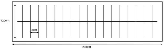
Figure 1. Schematic of the horizontal well and fracture stage configuration used in the numerical simulation.

The figure shows a top view of the model domain with dimensions of 2000 ft × 4200 ft and a fracture stage spacing of 80 ft. The horizontal wellbore is centered within the domain, and fracture stages are uniformly distributed along the well.

Each model that is studied has this configuration with the same well length, height, width, fracture length, and spacing. The different models are shown next.

The first model is the base case or the controlled model with no changes to it. It has a constant fracture permeability that does not change along the fracture length. The second model is supposed to represent a typical fracture model that uses the forward settling proppant method. The forward settling method creates higher fracture conductivity in the near-wellbore region. This is usually how Eagle Ford wells are fracked. The third is opposite the second and uses the reverse settling method, which places more proppant at the end of the fracture.

The rest of the models alter the average conductivity in the well and assume that some type of ceramic proppant is being used. This increases the conductivity in certain locations of the fracture. The fourth and fifth models are designed to test which fracture location would contribute more to the flow of the well. The fourth tests the two ends of the well with fracture stages 1, 2, 16, and 17. The fifth tests the middle of the well with fracture stages 7, 8, 10, and 11. The sixth and seventh models test the different ends of the half fracture lengths with increased conductivity. The sixth model focuses on increasing the conductivity at the tip of the fracture. The seventh model focuses on increasing the conductivity of the near-wellbore area.

2.6. Simulation Procedure and Field Benchmarking

The selection of 30-day and 1440-day simulation horizons reflects distinct reservoir flow regimes commonly observed in shale reservoirs. The 30-day period captures early-time transient and fracture-dominated flow behavior, which is frequently used in field practice to evaluate initial well productivity and completion effectiveness. The 1440-day simulation horizon represents longer-term reservoir drainage behavior, during which fracture interference and boundary effects become increasingly influential. Evaluating both time scales enables the assessment of fracture conductivity distribution effects on both short-term productivity and long-term cumulative production.

The data that was provided from the previous study measures a well based on its productivity index and does not specify the exact cumulative oil for the first 30 days.

However, from the cumulative production range of the production from 55 wells shown in Figure 2, the cumulative oil production is estimated around 16,500 barrels for the first 30 days [12].

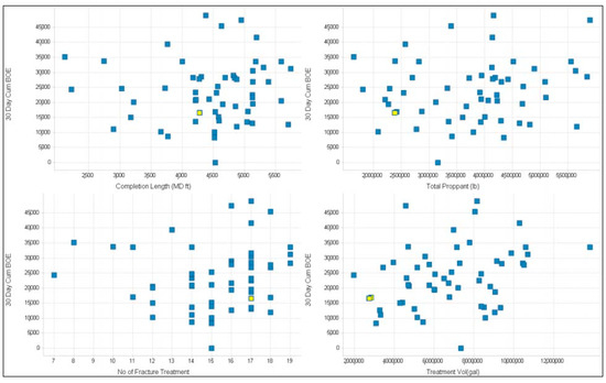
Figure 2. Cross-plots of 30-day cumulative oil production versus completion length, total proppant, number of fracture treatments, and treatment volume for Eagle Ford Shale wells.

After the data is created, all 6 models were run to collect the production data. Production data were then considered to see how accurate the simulation is when compared to the actual production.

In this study, the entire well length was run in the simulation for each model at 30 days and at 1440 days under the same conditions. This gave a good overall observation of what is happening specifically with fracture conductivity and how it affects the horizontal well. After the simulations were run, the daily flow rates, cumulative production, and productivity data were analyzed.

3. Results

3.1. Model Comparison with Field Data

The original field data yields an initial production rate of 16,500 barrels and a productivity index of 4.9 stb·day⁻¹·psi⁻¹. This is shown from the data collected from Robert Shelley in 2012 on the Eagle Ford Shale. This study helped greatly with setting up the simulation, but unfortunately, not all of the reservoir data was given. In the instance where data was not given, a typical Eagle Ford Shale value was assumed. This disconnect in some of the key pieces of data, such as the porosity and permeability of the reservoir, accounts for the difference in the cumulative rate and productivity index.

From the previous study, Luong determined that a single fracture was the optimum number of fractures for each stage. The model was compared to the field data mentioned earlier, and the productivity index of 6.3 stb·day⁻¹·psi⁻¹ from the single fracture per stage model was determined to be accurate for the well. In this study, the same single-fracture model with 17 stages is used. The productivity indexes are all with the range of six to eight stb·day⁻¹·psi⁻¹. This shows that the model used for simulation is in line with previously gathered field data.

The difference between the simulated and reported field productivity indexes reflects uncertainties associated with incomplete reservoir characterization and the use of representative parameter values. In this study, certain reservoir properties, such as porosity and permeability, were adopted as typical Eagle Ford Shale values due to limited availability of site-specific data. As a result, the model is not intended to reproduce exact field productivity values but to capture the overall production behavior and relative trends.

Despite the offset in absolute productivity index, the simulation reproduces the general production response and decline behavior observed in the field data. Moreover, the productivity indices obtained across different fracture conductivity scenarios fall within a relatively narrow range, indicating that the comparative conclusions of this study are not sensitive to moderate uncertainty in absolute parameter values.

3.2. Initial Production Data Analysis

The seven different models were run at a time step of one day for one month. This gives the 30-day initial production. This allows for the early time production to analyzed. The best metric to achieve this is the productivity index of the well, which shows how many barrels per day are produced per psi that the reservoir depletes. The highest productivity index for each model can be seen in Table 3.

Table 3. Highest productivity index in the first 30 days.

Model Number	1	2	3	4	5	6	7
Highest P. I in 30 Days (day−1·psi−1)	6.83	6.95	6.63	6.92	6.92	6.87	7.21

Before making conclusions about the P.I.s of the models, it is important to remember the physical differences between the models. Model 1 has constant conductivity with no change in the fracture. This model should be the baseline for all the models.

3.3. Model 2 and 3 Comparison of Forward vs. Backward Proppant Settling

Models 2 and 3 are the opposite versions of each other. Model 2 uses forward settling and is designed to show a higher conductivity near the wellbore and shrink towards the tip of the fracture. Model 3 uses backward settling for proppant and this performs the reverse of Model 2. The average for the total length of the fracture is 1529 mD for each of the first three models.

When comparing the P.I.’s of Models 2 and 3 to the base case of Model 1, the differences are +0.12 for Model 2 and −0.2 for Model 3. Before simulation, it was thought that the differences would be equal. This is not the case at all. Picture the fluid flow through the tip of the fracture; as it moves towards the wellbore, it encounters the different conductivities in the fracture. In Model 2, the fluid entering the fracture can flow much easier as it approaches the wellbore. This allows the well to produce more, thus giving the higher productivity index. In Model 3, as the fluid approaches the wellbore, the fluid is essentially chocked back or restricted. This causes the drop in productivity index.

The observed differences in productivity among the fracture conductivity scenarios can be explained by basic flow resistance considerations within the fracture. Higher fracture conductivity near the wellbore reduces pressure losses along the flow path, allowing hydrocarbons to enter the wellbore more efficiently and resulting in higher early-time production rates. In contrast, when fracture conductivity decreases toward the wellbore, flow encounters increased resistance as it approaches the well, effectively limiting the production rate.

These effects are evident in the comparison between Models 2 and 3, where enhanced near-wellbore conductivity leads to a higher productivity index than conductivity concentrated toward the fracture tip. This behavior highlights the importance of fracture conductivity distribution in controlling near-wellbore flow efficiency and early-time production performance.

3.4. Fracture Tip vs. Near-Wellbore Conductivity Enhancement (Models 6 and 7)

These two models are designed to test the productivity if a well has ceramic proppant, or an increased proppant conductivity, and where the best place to place that in a fracture would be. Model 6 places the ceramic proppant from the middle of the fracture to the tip. Model 7 places the proppant from the wellbore to the middle of the fracture. When observing the productivity indexes of the two models, it can be seen that both are more productive than the base case by +0.04 and +0.38, respectively. This increase in productivity can be attributed to the increase in average conductivity along the wellbore. Clearly, the better option of the two models is Model 7 with the improved fracture conductivity around the wellbore. Also, Model 6 shows that improving the tip of the fracture conductivity is not a lost cause. Model 7 is more economical than Model 6. The effects seen in Models 2 and 3 can also be seen here concerning the flow of oil.

3.5. Initial 30-Day Production Performance

The initial production behavior of the seven models is compared in Figure 3, where the wells with a higher fracture conductivity exhibit higher early-time oil rates. However, their decline is sharper during the first several days.

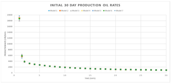
Figure 3. Initial 30-day oil production rates for all fracture conductivity distribution models.

The cumulative effect of these rate differences is shown in Figure 4, which illustrates the 30-day cumulative oil production for each model. Model 7 demonstrates the highest cumulative production, exceeding the base case by approximately 320 STB.

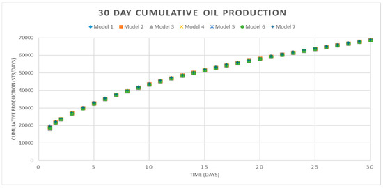
Figure 4. Thirty-day cumulative oil production for all fracture conductivity distribution models.

From the graphs it can be seen that initial production is crucial for these wells. Initially, the wells that have a higher average permeability will have a higher initial flow rate. The rates for the higher-conductivity wells dip below the base case after the first days of production. This happens because when the well begins to flow, the higher conductivity creates a larger pressure drop in the fracture, thus causing the following flow rates to be less than the lower-P.I. models. The cumulative production is ranked by which well has a higher P.I. The initial flow rate affects the P.I. much more than the following days and ensures that a larger P.I. will create a larger cumulative effect within the first thirty days of production. There is a difference between the models at the end of the 30 days. The largest is Model 7, with a difference of roughly 320 barrels.

3.6. Cumulative Production and Analysis

The cumulative oil production for all simulated models converges to approximately 320,000 bbl over the production life. While the overall cumulative production trends appear similar, additional insights are obtained by examining productivity index (P.I.) variations among the different fracture conductivity scenarios. Model 1 was selected as the reference case, and the difference in productivity index between each model and Model 1 was calculated and analyzed over time. The resulting comparisons are presented in Figure 5 and Figure 6.

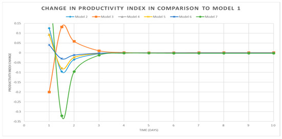
Figure 5. Change in productivity index relative to Model 1 during the first ten days of production, highlighting early-time fracture-dominated flow behavior.

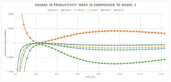
Figure 6. Change in productivity index relative to Model 1 from 10 to 1440 days of production, showing the convergence of long-term productivity trends.

Figure 5 illustrates the change in productivity index during the first ten days of production, highlighting early-time performance differences. Figure 6 presents productivity index variations from ten to 1440 days, with the y-axis centered at zero to emphasize relative changes with respect to Model 1. The absolute magnitude of the difference is not the focus; rather, attention is directed toward changes in curve direction and the occurrence of local maxima and minima, which reflect evolving reservoir drainage behavior.

Two notable transition points are observed in the productivity index trends. The first occurs approximately four days into production and corresponds to rapid depletion of hydrocarbons immediately surrounding the fracture, during which flow initially occurs in a near-radial manner. Following this period, production transitions to a slower decline as the drainage pattern shifts from three-dimensional flow to predominantly two-dimensional flow. The second transition occurs at approximately 215 days, when the drainage regions between adjacent fractures begin to overlap. Beyond this point, changes in productivity index become more gradual as the drainage area extends further into the surrounding reservoir.

At approximately 900 days of production, fracture drainage reaches the reservoir boundaries, after which cumulative production trends begin to converge across all conductivity scenarios. Although fracture conductivity distribution significantly influences production rates, particularly at early times, final cumulative production values remain similar across all models. These results illustrate the role of reservoir depletion and drainage evolution in governing long-term production behavior.

The reduced sensitivity of long-term cumulative production to fracture conductivity distribution can be attributed to the ultra-low-permeability nature of shale reservoirs. While fracture conductivity strongly controls early-time production by governing near-wellbore pressure drawdown and fracture-dominated flow, its influence diminishes over time as reservoir drainage expands beyond the immediate fracture vicinity. At later production stages, flow behavior is increasingly governed by matrix permeability and reservoir-scale pressure depletion rather than localized fracture conductivity variations.

The convergence of cumulative production trends observed across the different conductivity scenarios is therefore consistent with prolonged transient linear flow behavior commonly reported in shale reservoirs. Within the simulated time frame, the reservoir effectively behaves as infinite-acting, as boundary effects do not yet dominate production performance. This behavior is primarily attributed to the ultra-low matrix permeability and the relatively high fracture conductivity assumed in the model, under which pressure drop along the fracture is small during early production, making the infinite-acting flow assumption reasonable within the simulated time frame. This interpretation is consistent with published shale production studies and supports the observed long-term production behavior in the present analysis.

4. Conclusions

The objective of this study was to improve the understanding of fracture conductivity distribution and its influence on shale well production performance using numerical simulation. Based on the results obtained, the following conclusions can be drawn:

(1)

All simulation models produced production trends that are consistent with reported field-scale behavior, supporting the validity of the modeling approach.

(2)

Among the evaluated scenarios, Model 7 demonstrated the highest overall production performance, primarily due to its higher effective fracture conductivity distribution.

(3)

Fracture conductivity exhibits a limited influence on long-term cumulative production; however, modest changes in proppant placement and conductivity distribution can result in noticeable improvements in early-time production rates.

(4)

Within the scope of this study, fracture location along the horizontal well exhibits a limited influence on fracture conductivity performance and long-term cumulative production.

(5)

Higher-conductivity proppant placement in the near-wellbore region was observed to be more effective in enhancing early-time productivity under the simulated conditions.

(6)

Within the simulation time frame and modeling assumptions considered in this study, infinite-acting flow behavior dominates production due to the ultra-low permeability of the reservoir.

(7)

While proppant type was not explicitly modeled, the results suggest that higher-conductivity materials (e.g., ceramic proppants) may improve production performance when strategically placed near the wellbore or fracture tips.

(8)

Although fractures with different conductivity distributions reach similar drainage extents over time, the rate at which reservoir depletion occurs is influenced by fracture conductivity, particularly during early production stages.

5. Recommendations

To improve the model’s fidelity, future work should address several key areas. Generating a grid with sufficient resolution to capture micro-fractures accurately remains a significant challenge. While assuming a 0.25 ft wellbore radius was effective, future models should incorporate realistic fracture widths. Additionally, further study is needed to characterize better the overall geometry and shape of the fracture network.

References

- Chen, J.; Wang, L.; Wang, C.; Yao, B.; Tian, Y.; Wu, Y.-S. Automatic fracture optimization for shale gas reservoirs based on gradient descent method and reservoir simulation. Adv. Geo-Energy Res. 2021, 5, 191–201. [Google Scholar] [CrossRef]
- Hussain, M.; Boukadi, F. CO2-WAG Injection and Hysteresis Effects: Insights for Improved Oil Recovery and Carbon Sequestration Applications. Pet. Petrochem. Eng. J. 2025, 9, 000405. [Google Scholar] [CrossRef]
- Irogbele, A.B.; Ibrahim, B.A.; Adjei, D.; Amponsah, V.N.B.; Trabelsi, R.; Trabelsi, H.; Boukadi, F. Scale Deposition during Water Flooding and the Effect on Reservoir Performance. Processes 2025, 13, 2645. [Google Scholar] [CrossRef]
- Xu, C.; Li, P.; Lu, Z.; Liu, J.; Lu, D. Discrete fracture modeling of shale gas flow considering rock deformation. J. Nat. Gas Sci. Eng. 2018, 52, 507–514. [Google Scholar] [CrossRef]
- Zhang, H.; Zhao, H.; Jiang, M.; Pu, J.; Luo, Y.; Chen, W.; Luo, T.; Li, Z.; Yu, X. Estimated Ultimate Recovery and Productivity of Deep Shale Gas Horizontal Wells. Fluid Dyn. Mater. Process. 2025, 21, 221–232. [Google Scholar] [CrossRef]
- Luo, W.; Liu, P.; Tian, Q.; Tang, C.; Zhou, Y. Effects of discrete dynamic-conductivity fractures on the transient pressure of a vertical well in a closed rectangular reservoir. Sci. Rep. 2017, 7, 15537. [Google Scholar] [CrossRef] [PubMed]
- Sang, Y.; Guo, Y.; Huang, H.; Xia, D.; Chen, L.; Zhang, Z.; Gui, J. Experimental study on the long-term conductivity of self-support fracture in deep shale reservoirs. J. Pet. Explor. Prod. Technol. 2025, 15, 102. [Google Scholar] [CrossRef]
- Sadrpanah, H.; Dean, R.H.; Narr, W.; Settari, A. Explicit Simulation of Multiple Hydraulic Fractures in Horizontal Wells. In Proceedings of the SPE 99575, SPE Europec/EAGE Annual Conference and Exhibition, Vienna, Austria, 12–15 June 2006. [Google Scholar] [CrossRef]
- Khan, J.A.; Padmanabhan, E.; Haq, I.U. Hydraulic fracture conductivity in shale reservoirs. In Hydraulic Fracturing; Intech Open: London, UK, 2021. [Google Scholar] [CrossRef]
- Kong, C.; Sun, Y.; Zheng, D.; Li, Q.; Su, X.; Jia, Q.; Zhang, T.; Hou, J.; Dong, L.; Zhang, X.; et al. Analysis of the impact of CO2 injection on fracturing fluid flowback in shale gas wells. Sci. Rep. 2025, 15, 34223. [Google Scholar] [CrossRef] [PubMed]
- Meyer, E. Fracture conductivity prediction based on machine learning in shale—Part I. EarthArXiv 2024. [Google Scholar] [CrossRef]
- Shelley, R.; Saugier, L.; Al-Taiji, W.; Guliyev, N. Understanding Hydraulic Fracture Stimulated Horizontal Eagle Ford Completions. In Proceedings of the SPE 152533, SPE Conference and Exhibition, Vienna, Austria, 20–22 March 2012. [Google Scholar] [CrossRef]
Disclaimer/Publisher’s Note: The statements, opinions and data contained in all publications are solely those of the individual author(s) and contributor(s) and not of MDPI and/or the editor(s). MDPI and/or the editor(s) disclaim responsibility for any injury to people or property resulting from any ideas, methods, instructions or products referred to in the content. |
© 2026 by the authors. Licensee MDPI, Basel, Switzerland. This article is an open access article distributed under the terms and conditions of the Creative Commons Attribution (CC BY) license.