Abstract
Pipeline leakage is a common issue in many pressurized pipeline systems, with significant hazards, making it a current research hotspot. To reveal the fundamental characteristics of leakage in straight pipelines and 90° elbows transporting different media and thereby predict leakage locations, this paper conducts numerical calculations of the internal flow, while also predicting the pipeline leakage location monitoring model. The study finds that under air medium conditions, the nonlinear function model demonstrates excellent prediction accuracy, with R2 > 0.99 for the water3 condition. Under water medium conditions, the model’s fitting performance gradually weakens with increasing inlet pressure, with R2 dropping to 0.77. For a bent pipe, when air is used as the medium, the pressure peak at the large bend angle increases significantly under high inlet pressure. In contrast, when water is the medium, the local pressure reconstruction effect in the bent pipe exhibits a linear strengthening trend as the inlet pressure increases.
1. Introduction
Pipeline leakage detection technology has undergone an evolutionary process from single physical quantity monitoring to multimodal fusion. Early studies mainly relied on acoustic emission technology, locating leaks by capturing the pressure wave characteristics generated by leakage [1]. Although this method achieved certain results, its fault identification accuracy in practical applications is relatively low due to significant environmental noise interference. To address this issue, numerous scholars have conducted extensive research on the application of acoustic emission technology in pipeline leakage. Yao et al. proposed a spatiotemporal data-driven framework (STDDF) for natural gas pipeline leakage detection based on acoustic signals, which can effectively capture the temporal dynamic characteristics of leakage signals with a maximum fault identification accuracy of 99% [2]. Nguyen et al. used sensors deployed at both ends of the pipeline to estimate the time difference of arrival (TDOA) of acoustic emission (AE) events caused by leakage; the difference in propagation distance of each AE event was then calculated using the known wave propagation speed to determine the leakage position [3]. This method achieves high positioning accuracy with an error range of 0% to 1%. Saleem et al. converted AE signals from the time domain to scalogram images through continuous wavelet transform (CWT) to enhance leakage-related features [4], which significantly improved the detection and maintenance capabilities of urban pipelines. For pipeline leakage under multiple operating conditions, Yuan et al. adopted pixel-level image fusion technology and an evolutionary convolutional neural network (ECNN) improved by the whale optimization algorithm (WOA), converting traditional one-dimensional leakage time series into two-dimensional acoustic images containing richer information [5]. The optimized WOA-ECNN model exhibits significantly higher diagnostic accuracy than traditional CNN models.
With interdisciplinary integration becoming a mainstream trend, pipeline leakage monitoring technology has achieved multi-faceted development. To resolve the discrepancy between numerical simulation results and experimental measurement data under environmental influences, Duan studied the impact of different system uncertainties on the modeling and analysis of transient pipeline leakage flow, considering various factors of pipeline and fluid properties as well as system operations and complexity in the uncertainty analysis [6]. To address the challenge of multiphase flow, Adegboye et al. proposed a numerical method to investigate the influence of gas-liquid two-phase leakage flow behavior in subsea natural gas pipelines [7]. Their results indicate that flow field parameters provide relevant indicators for pipeline leakage detection: even for small leak sizes, upstream pipeline pressure can serve as a key indicator for leakage detection, while downstream flow rate is the main leakage indicator when flow monitoring is selected. Compared with traditional methods, machine learning has significantly improved the ability to detect small leaks. Roy applied a neural network method for leakage detection [8], introducing a weighted average localization algorithm to obtain the precise position of leakage points. The proposed hybrid neural network method remarkably enhances the accuracy of the pipeline leakage detection process, as evidenced by computational results, and minimizes the dilemma of complex decision-making. With the development of artificial intelligence technology, Rajasekaran et al. proposed a standalone leakage detection and localization architecture based on a single sensor, using a one-dimensional convolutional neural network (1DCNN) for feature extraction to realize leakage position detection and localization [9]. Behari et al. conducted key technical analysis and evaluation for chronic leakage detection under subsea and Arctic conditions, pointing out that dynamic pressure wave monitoring can identify medium and large leaks of 3–10 mm; sequential probability ratio test combined with real-time transient monitoring is suitable for multiphase flow leakage detection. Although distributed temperature and acoustic sensing using optical fiber cables is effective, it has high installation costs and operational risks [10]. Pipeline leakage detection technology has evolved from early acoustic emission to multimodal fusion, gradually overcoming noise interference and system uncertainties. By optimizing mechanism models, utilizing upstream and downstream pressure and flow rate changes, and integrating machine learning and artificial intelligence technologies, the ability of pipeline leakage detection and localization has been improved; dynamic monitoring and comprehensive models have also been introduced to enhance accuracy. Despite challenges such as high costs and the risks associated with existing technologies, the overall trend is moving toward higher efficiency and intelligence.
With the integration of interdisciplinary technologies, pipeline leakage detection has embarked on new directions. For example, Al-Ammari et al. achieved a breakthrough by constructing a digital twin (DT) framework for natural gas pipelines [11]. They developed a DT-based pipeline leakage detection model combined with machine learning technology, successfully realizing zero false alarm identification of leaks and accurate judgment of leakage position and size (error < 3.21%), providing a new method for pipeline safety monitoring. Xie et al. used nonlinearly coupled first-order hyperbolic partial differential equations to simulate actual pipelines [12]. Based on the linearization of water hammer equations, the Cayley–Tustin time discretization scheme was used to realize an infinite-dimensional hyperbolic PDE system without spatial approximation. A discrete Luenberger observer based on the algebraic Riccati equation was designed to reconstruct pressure and mass flow rate, and a support vector machine model was trained to detect leakage position and size. Simulations verified the effectiveness of the method, achieving precise leakage detection and localization. Asada et al. proposed a pipeline leakage detection method based on inverse transient analysis and comprehensive learning particle swarm optimization [13], which was successfully applied in an 18 km long irrigation pipeline system with an average leakage localization error of less than 1%, effectively reducing engineering inspection costs. Delgado-Aguiñaga et al. proposed a two-step method to identify pipeline network leakage parameters [14]: first, the leakage area is located through flow residual analysis, and then the extended Kalman filter is used to identify leakage parameters. This method simplifies observer design without traversing all possible leakage positions, making it suitable for complex pipeline network structures. Ahmad et al. proposed a pipeline leakage detection method based on acoustic emission signals and deep learning [15], generating acoustic images through wavelet transform, extracting global and local features by combining convolutional autoencoders and convolutional neural networks, and finally achieving high-precision leakage identification through a shallow neural network. For the special case of marine pipelines, Cui et al. proposed an improved leakage identification method by combining improved complete ensemble empirical mode decomposition with adaptive noise (ICEEMDAN) and probabilistic neural network (PNN) [16]. Compared with traditional analysis technologies, it exhibits outstanding performance in stability, anti-interference ability, and detection accuracy for marine pipeline detection. Regarding the complex gas–liquid two-phase flow mechanism in marine pipelines, Kam first proposed a mechanism modeling for leakage in long-distance horizontal subsea pipelines through pressure distribution calculation [17], presenting results in the form of contour maps. The results show that the outlet flow rate monitored at the receiving end can serve as a reliable indicator for leakage detection. On the basis of traditional pipeline leakage detection methods, Li et al. introduced an improved negative pressure wave method for optimization, combining the mass flow balance method and pressure change inflection point to realize pipeline leakage determination [18], effectively solving the problems of high false alarm rate, low positioning accuracy, and poor stability of traditional methods. Han et al. established an acoustic simulation model based on aeroacoustics principles and leakage flow field characteristics, starting from the generation mechanism of gas pipeline leakage sound sources [19], providing a theoretical basis for acoustic detection methods. Feng et al. studied the formation mechanism of disaster chains based on the chain characteristics of urban natural gas pipeline leakage processes using Markov chain theory [20], established an operational state evaluation system and quantified failure probability, thereby determining leakage causes and disaster-causing paths. The methods proposed by many scholars have significantly improved the accuracy and reliability of leakage detection, achieving comprehensive progress from leakage identification to precise localization. Meanwhile, integrating physical models, data-driven approaches, and optimization algorithms has further enhanced the understanding and prediction capabilities of leakage characteristics under complex operating conditions. Despite a series of advancements, the field still faces challenges such as data dependence on simulation, unsatisfactory computational efficiency, and the need for unified standardization.
Regarding future development directions and unresolved issues, current pipeline leakage detection research still confronts multiple challenges. To address the core problem of interaction between multiple leakage points, Rui et al. proposed a new mathematical model capable of detecting multiple leakage points in pipelines [21], realizing real-time identification of leakage positions and sizes through multi-flow tests, solving the misjudgment problem of traditional single-leakage assumption models in multi-leakage scenarios with advantages such as low computational cost and fast response. For transient start-up interference, Gao et al. proposed a time delay estimation algorithm based on differential process for pipeline leakage localization [22], enhancing high-frequency information and suppressing low-frequency interference by changing system characteristics. Compared with traditional cross-correlation and pre-whitening methods, it can obtain more reliable peaks and higher positioning accuracy. In response to the challenges of complex underwater transmission, Reda et al. reviewed the application status and challenges of subsea pipeline leakage detection technologies [23], emphasizing the need to distinguish between normal operating conditions and abnormal leakage events by integrating environmental, safety, and regulatory requirements, providing technical options and implementation guidance for pipeline integrity management. Vandrangi et al. systematically reviewed pipeline leakage detection, diagnosis, and prediction methods suitable for multiphase flow and transient operating conditions [24], comparing the advantages and disadvantages of model-driven and data-driven technologies, proposing the integration of multiple methods to improve detection accuracy, and providing practical guidance for diagnostic system design and research.
With the development of computational fluid dynamics (CFD), numerical calculation has become a highly effective method for studying pipeline leakage problems. Based on this, this study conducts numerical prediction on leakage scenarios in a straight pipeline and a 90° elbow transporting gas and liquid, respectively. The research not only obtains internal flow field characteristics but also focuses on achieving an accurate prediction of leakage positions.
2. Computational Model and Methodology
2.1. Computational Model
The first computational model is a straight pipe model with a geometric configuration of a standard cylindrical pipeline. The total length is set at 1000 mm, and the inner diameter is 100 mm. This parameter combination is designed to simulate typical long straight pipe flow scenarios, facilitating the analysis of velocity distribution, pressure drop characteristics, and flow stability of the fluid in the fully developed region.
The second model is a bent-pipe model. Its configuration consists of two straight pipe sections, each with a length of 900 mm and an inner diameter of 100 mm, connected by a standard 90° elbow. The elbow has a bend radius of 50 mm and the same inner diameter of 100 mm, forming a continuous flow channel. The elbow section smoothly connects the ends of the two straight pipes through a geometric transition, with a bend radius-to-pipe diameter ratio of 0.5.
2.2. Governing Equations
The SST k–ω (shear stress transport k–ω) model combines the excellent ability of the k–ω model to describe free shear flow and the performance of the k–ε model in the near-wall region, making it highly suitable for simulating the evolution of turbulent kinetic energy in complex flows. By introducing a blending function, the SST model integrates the high precision of the k–ω model in the near-wall region with the stability of the k–ε model in the free-stream region. Thus, it exhibits stronger adaptability and robustness in complex flow scenarios such as boundary layer separation, adverse pressure gradient flow, and rotational flow. Its core idea is to use the k–ω equations to capture the rapid changes in turbulent viscosity and shear stress in the near-wall region, while switching to the form of the k–ε equations in the region far from the wall. This reduces the dependence on free-stream conditions and avoids potential numerical instability issues of the k–ω model in the far field [25,26]. Therefore, the SST k–ω model is selected to effectively perform numerical simulation of the pipeline flow field.
Turbulent kinetic energy characterizes the kinetic energy of turbulent fluctuations, and its governing equation is as follows [27,28]:
where k is the turbulent kinetic energy (m2/s2), which characterizes the kinetic energy of turbulent fluctuations; μt is the turbulent viscosity (Pa·s), calculated by μt = ρk/ω; σk is the turbulent Prandtl number (a model constant, taken as 0.85); Pk is the turbulent kinetic energy production term (Pa/s), defined as Pk = μt (∇ U + (∇ U)T):∇ U; β* is a model constant (0.09).
The specific dissipation rate characterizes the intensity of the kinetic energy dissipation process in turbulence. Its physical meaning refers to the energy dissipation rate per unit turbulent kinetic energy. The governing equation for this parameter is as follows:
where ω is the specific dissipation rate (1/s), which characterizes the ratio of turbulent dissipation rate to k; σω is the turbulent Prandtl number (a model constant, taken as 0.5 in the near-wall region and 0.856 in the far-field region); γ is the model coefficient (dynamically adjusted by the blending function F1); β is a model constant (taken as 0.075); and F1 is the blending function that controls the switching between the near-wall and free-stream models.
2.3. Mesh Generation
The mesh model diagram is shown in Figure 1a. For a straight pipeline, the results of mesh convergence verification are shown in Figure 1b. When the number of mesh elements reaches 2.5 × 10⁶, the fluctuation amplitude of the monitored velocity with mesh density has significantly attenuated to an acceptable range, meeting the mesh independence criterion. This phenomenon indicates that further increasing mesh density leads to saturated improvements in calculation results, and the proportion of discretization error has decreased to the threshold allowed by numerical simulation.
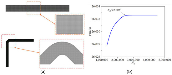
Figure 1.
Mesh model and grid independence verification: (a) mesh model; (b) grid independence verification.
For the bent-pipe model, since its total length is approximately twice that of the straight pipe model and the flow characteristic scale is more refined, increasing mesh density is necessary to adequately resolve the flow details in the elbow section and ensure controllable discretization errors in curvature-dominated regions. Therefore, the mesh count for the bent-pipe model is chosen to be above 5 × 10⁶. This setting effectively balances computational accuracy with resource consumption, enabling key monitoring parameters to achieve numerical stability in curved regions at a convergence level consistent with that of the straight pipe model.
The mesh configuration of the straight pipe adopts a layered composite mesh strategy. Its core feature is the use of polyhedral meshes in the near-wall region to enhance the resolving capability of boundary layer flow characteristics, while hexahedral meshes are employed inside the flow channel to improve computational efficiency and numerical stability. The boundary layer region achieves high-resolution capture of near-wall velocity gradients through polyhedral meshes. The number of mesh layers and thickness distribution are adaptively adjusted according to Reynolds number characteristics and wall shear stress distribution to ensure that the y+ value falls within the applicable range of the turbulence model. For the internal hexahedral meshes, uniform mesh spacing is maintained along the flow direction to reduce the accumulation of discretization errors, while a periodic encryption strategy is adopted in the transverse direction to match the resolution transition of the boundary layer meshes. Mesh orthogonality, as a core indicator of mesh quality, has its global minimum strictly controlled above 0.5.
2.4. Boundary Conditions
The boundary condition settings for the experimental conditions using air and water as test fluids follow the fundamental principle of pressure-driven flow. When air is used as the test medium, the inlet boundary is set as a pressure inlet, with initial pressure gradients of 1.0145 × 10⁵ Pa (Air1), 1.0150 × 10⁵ Pa (Air2), and 1.0155 × 10⁵ Pa (Air3). The outlet boundary is configured as a pressure outlet with an initial pressure of 1.0140 × 10⁵ Pa, while the leakage hole boundary pressure is set to the standard atmospheric pressure of 1.01325 × 10⁵ Pa. When water is used as the test medium, the inlet pressure gradients are adjusted to 1.0200 × 10⁵ Pa (Water1), 1.0400 × 10⁵ Pa (Water2), and 1.0600 × 10⁵ Pa (Water3), while the outlet boundary conditions remain consistent with those of the air test cases. This pressure gradient design aims to drive fluid motion by controlling the pressure difference between the inlet and outlet, while ensuring comparability in the Reynolds number range across different test conditions.
For the test conditions distinguishing between straight pipe and bent-pipe models, the bent pipe is tested only under air flow with an inlet pressure of 1.0150 × 10⁵ Pa (Air2). All other boundary conditions remain identical to those of the straight pipe case to eliminate interference from boundary condition differences in flow structure resolution. The arrangement of test holes is designed based on the spatial distribution characteristics of the flow feature scale and pressure gradient field. For the straight-pipe section, the test holes are symmetrically distributed along the axial direction, with the centerline distance from the inlet face increasing in 100 mm increments from 100 mm to 900 mm, forming a total of nine equally spaced measurement points. This layout effectively captures the transition region from developing flow to fully developed flow. For the bent-pipe section, the arrangement of test holes takes into account both the curvature-induced secondary flow structure and the non-uniformity of the pressure gradient field. Axially, the test points include 16 equally spaced locations: from 100 mm to 800 mm (at 100 mm intervals) on the inlet side and from 100 mm to 800 mm (at 100 mm intervals) on the outlet side. Additional characteristic test holes are added at symmetric center positions on the geometric centerline of the curved section and at the tangent points of the inner/outer arcs, resulting in a total of 18 test points. The diameter of all test holes is uniformly set to 5 mm to minimize flow disturbance, while reference tests under non-leakage conditions are retained to validate the influence mechanism of leakage effects on flow characteristics.
The spatial distribution number diagram of test holes is shown in Figure 2, and this layout design can systematically obtain the spatial evolution law of the pressure gradient field in the straight pipe. This figure illustrates all potential leakage hole locations to be simulated. Each simulation case involves only one leakage hole.
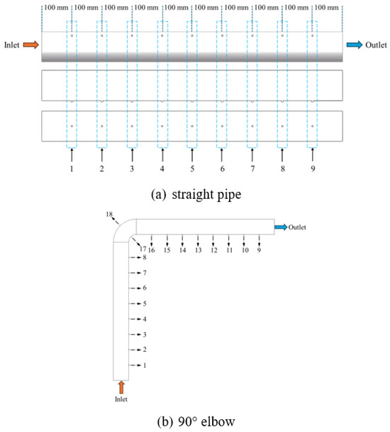
Figure 2.
Schematic diagram of leakage hole position. The numbers represent the locations of the monitoring points.
2.5. Vortex Identification
There are three definition methods for vortices: Q, Δ, and Ω criteria. Among them, Jinhee et al. proposed defining the region with Q > 0 as a vortex, where rotation dominates over strain rate in the vortex region, which is referred to as the Q criterion [29].
When Q > 0, rotation dominates the flow. It is decomposed based on the velocity gradient tensor , which can be split into a symmetric tensor A and an antisymmetric tensor B, representing the deformation and rotation at a point in the flow field, respectively. The expression is as follows:
The Q criterion is based on the second invariant of the velocity gradient tensor, and its expression is as follows:
where denotes the Frobenius norm of the matrix [30].
3. Straight Pipe
3.1. Internal Flow Field
To systematically observe the spatial distribution characteristics of the velocity field at the outlet surface in the presence of a leakage hole, a layout of representative monitoring points was set on the outlet cross-section, as shown in Figure 3. This layout takes the outlet center as the coordinate origin, selects the intersection points of the circumferential contour line with the coordinate axes along the vertical and horizontal directions, and arranges monitoring points 1 mm near the origin. This position selection balances the attenuation law of the wall effect and the velocity gradient characteristics of the central main flow region.
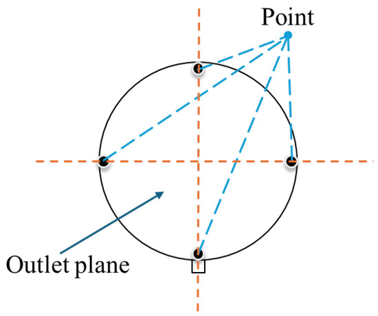
Figure 3.
Schematic diagram of monitoring point positions at the outlet.
The operating condition with the leakage hole 900 mm away from the outlet was selected for characteristic analysis. This distance corresponds to the fully developed flow region of the straight pipe section. If significant velocity distribution characteristics can still be observed at this far-field position, it can be inferred that the outlet surface under all leakage hole positions exhibits the same velocity field evolution law. The velocity states of the outlet cross-section under various operating conditions are shown in Figure 4, where Figure 4a–c correspond to the velocity distributions of air medium under inlet pressures of Air1 (1.0145 × 10⁵ Pa), Air2 (1.0150 × 10⁵ Pa), and Air3 (1.0155 × 10⁵ Pa), respectively; Figure 4d–f correspond to the velocity distributions of water medium under inlet pressures of Water1 (1.0200 × 10⁵ Pa), Water2 (1.0400 × 10⁵ Pa), and Water3 (1.0600 × 10⁵ Pa), respectively.
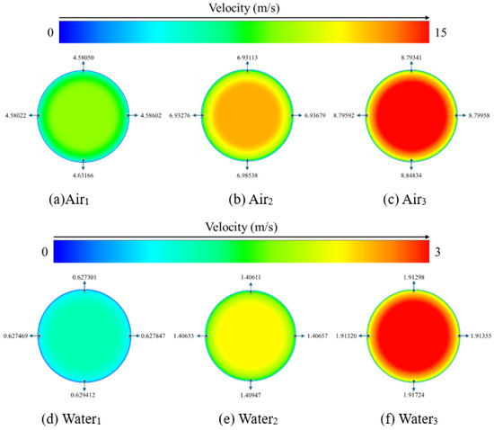
Figure 4.
Velocity values at the outlet position.
The results indicate that when the test fluid is air, the outlet velocity fields under the three inlets’ pressure gradients all exhibit significant inhomogeneous distribution characteristics: the velocity in the central region of the outlet cross-section is consistently higher than that in the edge region, and the velocity in the lower part of the edge region is significantly different from that in the upper part. Specifically, the velocities in the central region under Air1 to Air3 operating conditions are 4.63 m/s, 6.99 m/s, and 8.85 m/s, respectively, while the velocity in the lower part of the edge region is higher than that of other parts by 0.05 m/s (from 4.58 to 4.63), 0.06 m/s (from 6.93 to 6.99), and 0.05 m/s (from 8.80 to 8.85), respectively. For the water medium operating conditions, the outlet velocity field also shows similar asymmetric distribution characteristics: the velocities in the central region under Water1 to Water3 operating conditions are 0.627 m/s, 1.406 m/s, and 1.913 m/s, respectively, while the velocity in the lower part of the edge region is higher than that of other parts by 0.002 m/s (from 0.625 to 0.627), 0.003 m/s (from 1.403 to 1.406), and 0.004 m/s (from 1.909 to 1.913), respectively. Notably, the velocity in the lower part is always higher than that in other directions of the axis of symmetry, and this direction is exactly consistent with the geometric position of the leakage hole. This phenomenon indicates that the presence of the leakage hole induces the asymmetric reconstruction of the velocity field at the outlet cross-section, whose root cause can be attributed to the local pressure gradient disturbance and mass flux redistribution caused by the leakage hole. The above velocity distribution characteristics are highly consistent in both air and water medium operating conditions, verifying the universality of the regulatory effect of the leakage hole on the outlet flow field and providing a key theoretical basis for the subsequent development of leakage detection methods based on velocity field characteristics.
To systematically analyze the spatial evolution characteristics of the flow field in the presence of a leakage hole, a three-dimensional monitoring system was established on the axisymmetric plane of the pipeline (see Figure 5). The monitoring surface is defined as the longitudinal section passing through the pipeline axis, the monitoring line is a horizontal equidistant line 1 mm away from the leakage hole wall, and the monitoring points are selected in the characteristic region of the monitoring line near the outlet. The velocity values are calculated as the average of the velocities of the nearest 5 nodes along the flow direction in this region to eliminate the interference of local discretization errors on flow field characteristic identification.
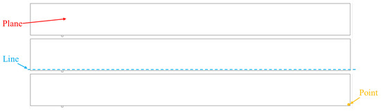
Figure 5.
Schematic diagram of monitoring surface, monitoring line, and monitoring points on the axisymmetric plane.
For air medium operating conditions, Figure 6 shows the distribution law of velocity contour maps on the monitoring surface under different inlet pressure gradients: Figure 6a–c correspond to velocity contour maps under low, medium, and high inlet pressures (Air1 to Air3), respectively, with the left boundary as the inlet end. The results indicate that regardless of the axial position of the leakage hole, the velocity field in the monitoring surface exhibits typical boundary layer development characteristics—from the inlet to the outlet, the velocity gradient in the central region of the pipeline continues to increase, while the velocity gradient near the wall region gradually decreases. This phenomenon is highly consistent under the three inlets’ pressure operating conditions. Specifically, under low, medium, and high inlet pressures, the maximum velocity in the central region of the outlet reaches 8.0 m/s, 12.0 m/s, and 14.0 m/s, respectively, while the velocity in the edge region at the corresponding position is only about 5.0 m/s, 7.0 m/s, and 9.0 m/s. The velocity gradient distribution shows a significant difference between the central main flow region and the near-wall layer. Further analysis reveals that when the leakage hole moves toward the inlet end, the density of velocity contours in the neighborhood of the leakage hole increases significantly, indicating an inhomogeneous enhancement of local flow velocity. This root cause can be attributed to local pressure gradient disturbance and mass flux redistribution induced by the leakage hole. The evolution law of the velocity field shows scale similarity under the three inlets’ pressure operating conditions, verifying the universality of the regulatory effect of the leakage hole on the flow field structure and providing a key theoretical basis for the subsequent research on leakage location methods based on velocity gradient distribution characteristics.
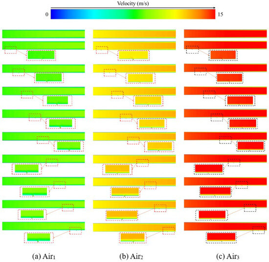
Figure 6.
Velocity contour maps of air fluid.
For the flow field evolution characteristics under water medium operating conditions, further analysis of the velocity field on the monitoring surface was conducted, as shown in Figure 7. Figure 7a–c correspond to velocity contour maps under low, medium, and high inlet pressures (Water1 to Water3), respectively, with the left boundary still as the inlet end. The results indicate that regardless of the axial position of the leakage hole, the velocity field in the monitoring surface exhibits typical boundary layer development characteristics—from the inlet to the outlet, the velocity gradient in the central region of the pipeline continues to increase, while the velocity gradient near the wall region gradually decreases. This phenomenon is highly consistent under the three inlets’ pressure gradients. Specifically, under low, medium, and high inlet pressures, the maximum velocity in the central region of the outlet exceeds 1.0 m/s, 2.0 m/s, and 2.8 m/s, respectively, while the velocity in the edge region at the corresponding position is only about 0.62 m/s, 1.40 m/s, and 1.90 m/s. The velocity gradient distribution also shows a significant difference between the central main flow region and the near-wall layer. Notably, when the leakage hole moves toward the inlet end, the density of velocity contours in the neighborhood of the leakage hole increases significantly, indicating an inhomogeneous enhancement of local flow velocity. This root cause can be attributed to local pressure gradient disturbance and mass flux redistribution induced by the leakage hole. The evolution law of the velocity field shows scale similarity under the three inlets’ pressure operating conditions, verifying the universality of the regulatory effect of the leakage hole on the flow field structure and providing a key theoretical basis for the subsequent research on leakage location methods based on velocity gradient distribution characteristics. It is particularly noteworthy that compared with air medium, the velocity gradient distribution under water medium shows a gentler evolution trend, which is closely related to the physical property that the dynamic viscosity coefficient of water is significantly higher than that of air. However, the overall flow field reconstruction mechanism still follows the same basic principles of fluid mechanics.
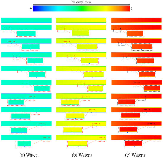
Figure 7.
Velocity contour maps of water fluid.
For the evolution characteristics of the vorticity field in the neighborhood of the leakage hole for air and water media, the significant differences in hydrodynamic behavior were revealed through vorticity contour map analysis. As shown in Figure 8, the vorticity distribution of air fluid on the monitoring surface exhibits highly localized characteristics: all vortex structures are concentrated at the leakage hole position, and no significant vorticity accumulation is observed in other regions. Notably, the vorticity magnitude at the leakage hole under the air medium can reach more than 6 × 10⁵ s−2 in the central region. This order of magnitude indicates that under the condition of air’s low viscosity coefficient (approximately 1.8 × 10⁻⁵ Pa·s), the local pressure gradient disturbance induced by the leakage hole can excite high-vorticity vortex structures. Further observation shows that the vorticity field is axially symmetric around the center of the leakage hole, and its intensity attenuation law follows the free vortex theory model—the vorticity magnitude is inversely proportional to the radius. This contradicts the irrotational characteristic of free vortices, suggesting that the coupling effect of viscous forces and inertial forces dominates the formation mechanism of vortex structures in actual flow.
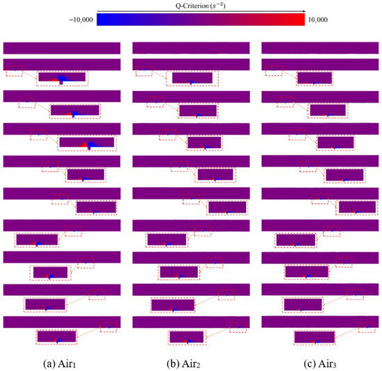
Figure 8.
Vorticity contour maps of air fluid.
In contrast to the water medium operating conditions (see Figure 9), the vorticity distribution shows significant scale differences: the vorticity magnitude in the central region of the leakage hole is only 1 × 10⁵ s−2, and it drops sharply to the order of hundreds of s−1 at the other wall of the pipeline. This phenomenon can be attributed to the fact that the dynamic viscosity coefficient of water (approximately 1.0 × 10⁻³ Pa·s) is two orders of magnitude higher than that of air, leading to the rapid suppression of vortex structures by viscous dissipation during their formation. More notably, the vorticity field under water medium exhibits asymmetric distribution characteristics—the maximum vorticity is located at the center of the leakage hole, but the attenuation rate toward the other side of the pipeline is significantly faster than that of the air medium. This asymmetry may originate from the synergistic effect of mass flux redistribution induced by the leakage hole and wall shear stress. The scale differences and distribution patterns of the vorticity field verify the dominant role of viscous forces in vortex structure evolution, whose physical essence can be traced back to the regulatory mechanism of viscous terms in the Navier–Stokes equations on flow separation and vortex generation. The above vorticity field characteristics provide a key theoretical basis for the mechanism research on flow field reconstruction induced by leakage holes, and simultaneously reveal the scale dependence of fluid physical parameters on vortex dynamic behavior.
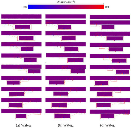
Figure 9.
Vorticity contour maps of water fluid.
Under air medium conditions, the regulatory effect of different leakage hole positions on the velocity field along the monitoring line exhibits significant spatial heterogeneity. Figure 10 shows the evolution law of velocity distribution along the monitoring line under different leakage hole positions, and the velocity field response presents typical inhomogeneous distribution characteristics. The local disturbance effect induced by the leakage hole at the axial position of 100 mm is particularly significant, manifested as an obvious gradient jump of the velocity curve at this position. The amplitude of this velocity fluctuation has a strong coupling relationship with the axial distribution of the leakage hole, and its numerical range shows a phased increasing trend within the intervals of 4.3~7.9 m/s, 6.8~11.3 m/s, and 8.5~13.9 m/s. Notably, a secondary enhancement effect of the velocity field can be observed in the downstream region of the leakage hole (near the outlet direction), with a flow velocity increase of up to 4 m/s. This maximum increase value is stable under different pressure gradients and leakage hole layout conditions. This velocity jump phenomenon can be attributed to the local release of kinetic energy of the main fluid by the leakage hole, and its energy conversion mechanism is consistent with the momentum conservation principle described by Bernoulli’s equation.
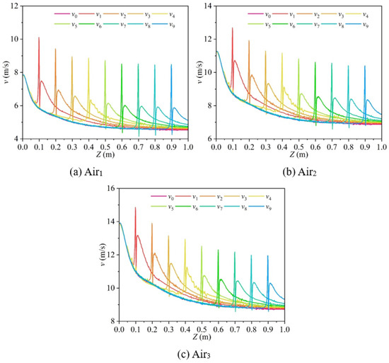
Figure 10.
Velocity variations along the monitoring line (Air).
For the water medium (Figure 11), the evolution law of the velocity field along the monitoring line also exhibits spatial dependence characteristics. Although the amplitude of velocity fluctuation differs by an order of magnitude from that of the air medium (0.62~0.99 m/s, 1.40~2.08 m/s, and 1.90~2.79 m/s), the regulatory effect of the leakage hole on the flow field still shows similar topological characteristics. When the leakage hole is 100 mm away from the inlet, the velocity curve along the monitoring line also exhibits significant fluctuation at this position, and the flow velocity in the downstream region shows a phased increasing trend. However, significantly different from the air medium, the leakage hole in water fluid does not induce a flow velocity increase exceeding the inlet velocity (the maximum increase is only 0.2 m/s). This difference can be attributed to the damping effect of water’s high viscosity on velocity field diffusion and the constraint effect of the incompressibility of the liquid medium on energy dissipation. Data further indicate that the functional relationship between the fluctuation amplitude of the water velocity field and the leakage hole position still follows an increasing law similar to that of the air medium, but the magnitude of the increase is limited by the physical parameters of the liquid medium. This comparative study on cross-medium flow field response characteristics provides an important theoretical basis for the medium adaptability design of leakage detection technologies.
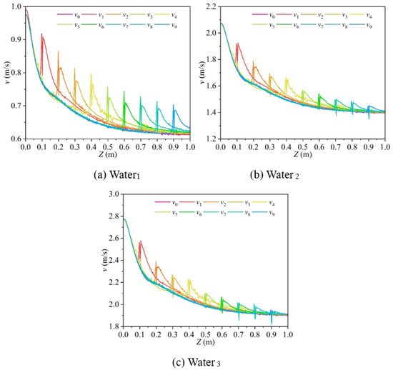
Figure 11.
Velocity variations along the monitoring line (water).
3.2. Prediction Functions
The velocity values near the outlet along the monitoring line show significant nonlinear response characteristics with changes in the leakage hole position. To systematically analyze this spatial dependence, a functional model between velocity and leakage position was established, and the polynomial regression method was adopted for fitting. Based on the simulation data, three sets of functional models were constructed, denoted as f1, f2, and f3.
The f1 equation is as follows:
where A1, A2, and A3 are coefficients to be fitted, and A0 is the constant term to be fitted.
The f2 equation is as follows:
where B1, B2, B3, and B4 are coefficients to be fitted, and B0 is the constant term to be fitted.
The f3 equation is as follows:
where C1, C2, and C3 are coefficients to be fitted, and C0 is the constant term to be fitted.
To evaluate the fitting results, the coefficient of determination (R2) of the fitting curve was calculated. R2 is one of the statistical indicators to measure the goodness of fit of the regression model. It represents the proportion of the variation in the dependent variable that can be explained by the independent variable, and its calculation formula is as follows:
where is the original efficiency data, is the average value of the original efficiency data, and is the fitted data value.
R2 measures the degree of variation in the dependent variable that the model can explain, with a value range between 0 and 1. A higher R2 indicates that the model can fit the data well, while a lower R2 indicates poor fitting performance.
For the Air1 condition, the f1, f2, and f3 equations are as follows:
The point monitoring and fitting results for Air1 are shown in Figure 12. The R2 values of f1, f2, and f3 are 0.99785, 0.99831, and 0.99932, respectively, indicating that the models can highly reproduce the spatial distribution characteristics of the velocity field with minimal deviation between the fitting curves and the simulation data. This phenomenon can be attributed to the low viscosity of air, which endows the evolution law of the velocity field with strong determinism and predictability.
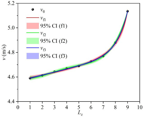
Figure 12.
Point monitoring and fitting results for Air1.
For the Air2 condition, the f1, f2, and f3 equations are as follows:
The R2 values of f1, f2, and f3 are 0.99725, 0.99798, and 0.99882, respectively.
The point monitoring and fitting results for Air2 are shown in Figure 13. The R2 values remain at a high level. Although slightly lower than those for Air1, the values are still close to 1, indicating that the model’s ability to describe the velocity field is not significantly affected.
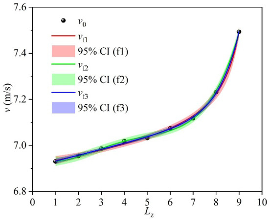
Figure 13.
Point monitoring and fitting results for Air2.
For the Air3 condition, the f1, f2, and f3 equations are as follows:
The point monitoring and fitting results for Air3 are shown in Figure 14. The R2 values of f1, f2, and f3 further increase to 0.99854, 0.99618, and 0.99921, respectively, demonstrating the model’s adaptability to complex flow structures. Notably, the R2 value of f2 is slightly lower than that in the previous two conditions, indicating that the quartic polynomial model may not be the optimal choice under Air3 conditions, while the cubic polynomial models f1 and f3 exhibit more stable fitting performance.
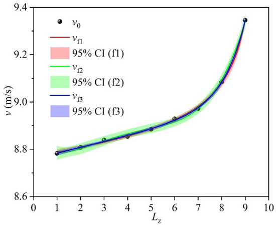
Figure 14.
Point monitoring and fitting results for Air3.
For the Water1 condition, the f1, f2, and f3 equations are as follows:
The point monitoring and fitting results for Water1 are shown in Figure 15. The R2 values of f1, f2, and f3 are 0.99518, 0.99205, and 0.99662, respectively. In comparison, the R2 values of the three models under the water medium are generally lower than those under the air medium. For Water1, although the fitting performance is slightly inferior to that of air medium, it still remains within the high-precision range.
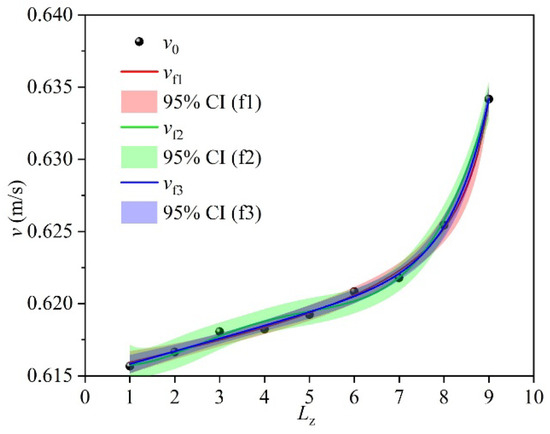
Figure 15.
Point monitoring and fitting results for Water1.
For the Water2 condition, the f1, f2, and f3 equations are as follows:
The point monitoring and fitting results for Water2 are shown in Figure 16. For Water2, the R2 value of f1 decreases significantly to 0.92243, and obvious fitting distortion occurs at leakage position 7. The error is mainly due to the failure of the model to fully capture the nonlinear disturbances of the local velocity field.
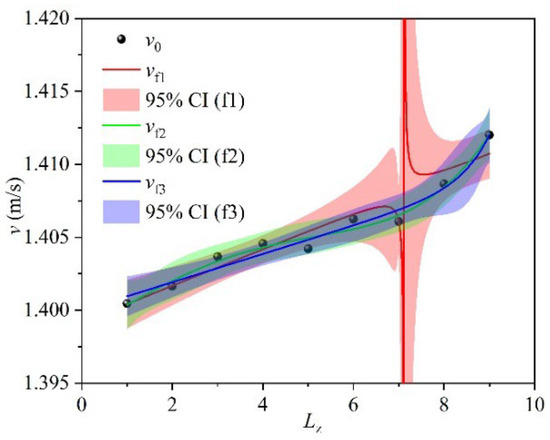
Figure 16.
Point monitoring and fitting results for Water2.
For the Water3 condition, the f1, f2, and f3 equations are as follows:
The point monitoring and fitting results for Water3 are shown in Figure 17. For Water3, the R2 values drop to 0.90485, 0.83783, and 0.77016, indicating a significant weakening of the model’s fitting ability. This phenomenon can be attributed to the damping effect of water’s high viscosity and low compressibility on velocity field diffusion, which makes the variation characteristics of the measured data tend to be gentle, thereby reducing the explanatory power of the model.
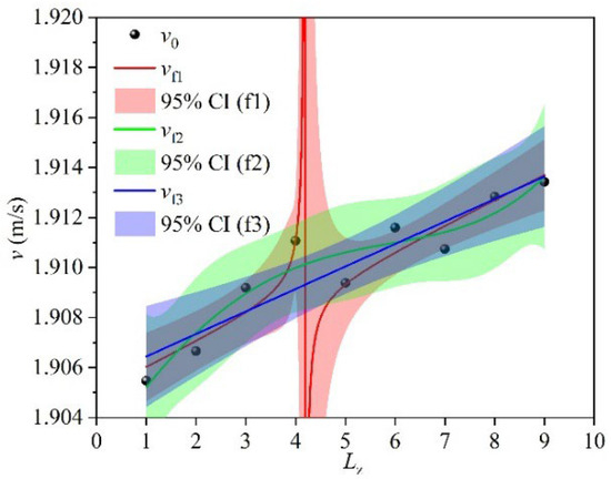
Figure 17.
Point monitoring and fitting results for Water3.
In summary, the constructed nonlinear function models exhibit excellent fitting performance under air medium conditions, with R2 values generally higher than 0.99. This verifies the models’ high-precision descriptive ability for the spatial evolution law of the velocity field. For water medium systems, the applicability of the models is significantly affected by fluid physical parameters. In particular, under operating conditions with weakened flow characteristics, it is necessary to optimize the model structure by integrating other physical mechanisms (such as viscous dissipation or turbulent effects) to improve prediction accuracy.
4. 90° Elbow
4.1. Velocity Contour
The distribution characteristics of the fluid velocity field and the evolution patterns of vortex structures in the axisymmetric plane of a curved pipe exhibit a significant dependence on the location of leakage holes. Figure 18 presents velocity contour maps for three scenarios: no leakage hole, leakage hole located on the inner side of the bend, and leakage hole located on the outer side of the bend. The velocity range covers 0 to 15 m/s. On the inner side of the bend, due to centrifugal acceleration along the curved path, the local velocity can reach up to 15 m/s. In contrast, in the outer bend region, where the fluid path is longer and viscous dissipation is more pronounced, the velocity decreases to approximately 5 m/s.
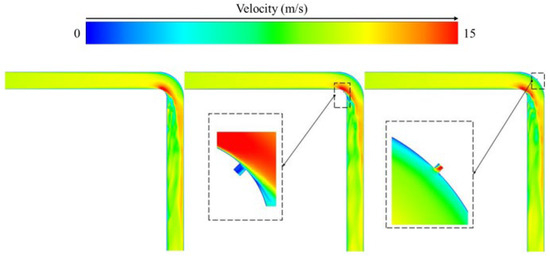
Figure 18.
Velocity contour for the case without a leakage point and for cases with leakage points located at the bend.
When the leakage hole is located on the inner side, despite the higher flow velocity in the inner bend region, the fluid does not exit significantly through the leakage hole due to the angle between the leakage direction and the main flow direction. Only minor local disturbances are observed. Conversely, when the leakage hole is located on the outer bend, where the flow velocity is lower and more stable, the presence of the leakage hole also does not significantly alter the overall velocity field distribution.
Therefore, the differences among the velocity contour maps for the three cases are relatively small, indicating that the influence of leakage hole location on the overall velocity field in the curved pipe is limited. This phenomenon can be attributed to the compensatory effect between the high-speed flow in the inner bend and the low-speed flow in the outer bend under the influence of leakage holes. As a result, no significant mass transfer or energy dissipation occurs in the fluid.
Figure 19 further analyzes the evolution characteristics of the velocity field when leakage holes are located at the inlet-side positions of the straight pipeline (positions 1–8).
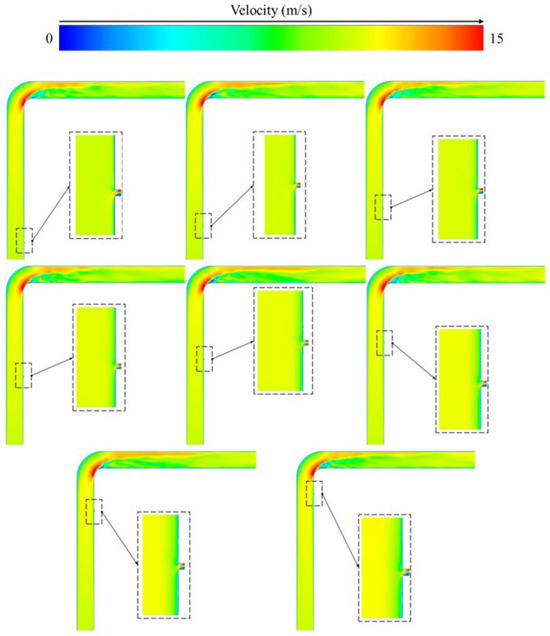
Figure 19.
Velocity contour when leakage points are located at positions 1–8.
The figure shows that the fluid velocity distribution in the straight pipe section before entering the bend is relatively uniform. However, after passing through the bend, the flow structure undergoes significant changes. The velocity contours near the bend exit exhibit evident chaotic features, with increased velocity gradients in local regions and even the occurrence of reverse flow. This phenomenon can be attributed to the acceleration of fluid on the inner side of the bend due to centrifugal forces, while the fluid on the outer side decelerates due to the extended flow path. The velocity difference between these two regions induces secondary flows, leading to enhanced non-uniformity in the velocity field. Moreover, the presence of leakage holes further exacerbates flow instability. The local velocity disturbances near the leakage holes interact with the secondary flows generated in the bend, resulting in a more complex velocity field distribution. However, when the leakage holes are located near the inlet of the straight pipe section, the impact on the downstream velocity field of the bend remains relatively limited. The primary effect is localized velocity disturbances, without significantly altering the overall flow structure.
Figure 20 illustrates the velocity field characteristics when leakage holes are located at the outlet-side positions of the straight pipeline (positions 9–16). Similar to Figure 19, the velocity distribution of the fluid after entering the bend also exhibits significant chaotic features. However, due to the proximity of the leakage holes to the bend exit, their influence on the flow is more direct. Near the bend exit, the presence of leakage holes leads to localized fluid mass loss, resulting in an asymmetric distribution of the velocity field at the outlet end. Specifically, the high-speed flow on the inner side of the leakage holes weakens due to mass loss, while the low-speed flow on the outer side slightly intensifies due to a shortened flow path. This redistribution of the velocity field further exacerbates the flow separation phenomenon near the bend exit. Additionally, the change in leakage hole location prolongs the recovery time of the velocity field in the straight pipe section downstream of the bend, reducing its velocity uniformity compared to the scenario without leakage. This phenomenon indicates that the location of leakage holes not only affects the flow characteristics within the bend but also alters the flow recovery process downstream of the bend through mass transfer effects.
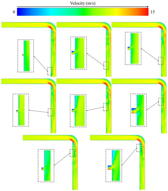
Figure 20.
Velocity contour when leakage points are located at positions 9–16.
4.2. Vortex Distribution
Figure 21 reveals the evolution of vortex distribution in the presence of leakage holes simultaneously on both the inner and outer sides of the bend. In the scenario without leakage, stable secondary flows are formed on the inner side of the bend due to centrifugal force, with vortex structures primarily concentrated at the bottom of the inner bend and the top of the outer bend. When leakage holes are located on the inner side, the vortex intensity decreases significantly. This occurs because the presence of leakage holes allows a portion of the high-speed fluid flow on the inner side to escape, thereby weakening the driving capability of the secondary flow on the inner side. In contrast, leakage holes on the outer bend have a lesser impact on the vortex structure, causing only slight fluctuations in vortex intensity in localized regions. This phenomenon indicates that the flow structure on the inner side of the bend is more sensitive to the presence of leakage holes, while the low-speed flow on the outer side is relatively less affected by disturbances from leakage holes. Furthermore, changes in the location of leakage holes lead to a shift in vortex distribution downstream of the bend exit, with its intensity exhibiting a nonlinear variation trend as the leakage hole position changes.
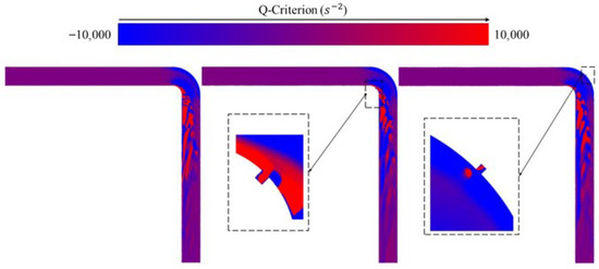
Figure 21.
Vortex distribution for the case without leakage points and for cases with leakage points located at the bend.
Figure 22 details the vortex distribution characteristics when leakage holes are located in the inlet section of the straight pipeline (positions 1–8). In the scenario without leakage, the vortex intensity is highest on the inner side of the bend, with a vortex core diameter of approximately 2 mm, and the vortex structures are continuously distributed along the bottom of the inner bend. When leakage holes are introduced, the vortex intensity at their locations significantly increases, with the local vortex core diameter expanding to about 5 mm, indicating that the presence of leakage holes exacerbates flow instability in these regions. However, the influence of the leakage holes on the vortex distribution downstream of the bend is relatively minor. The vortex structures remain predominantly concentrated at the bottom of the inner bend and the top of the outer bend, with no significant changes observed in their intensity distribution. This phenomenon can be attributed to the proximity of the leakage holes to the inlet of the straight pipe section, where their disturbance effects have not yet fully propagated to the downstream regions of the bend. Furthermore, the strong vortex structures near the leakage holes interact with the secondary flow on the inner side of the bend, forming localized vortex clusters.
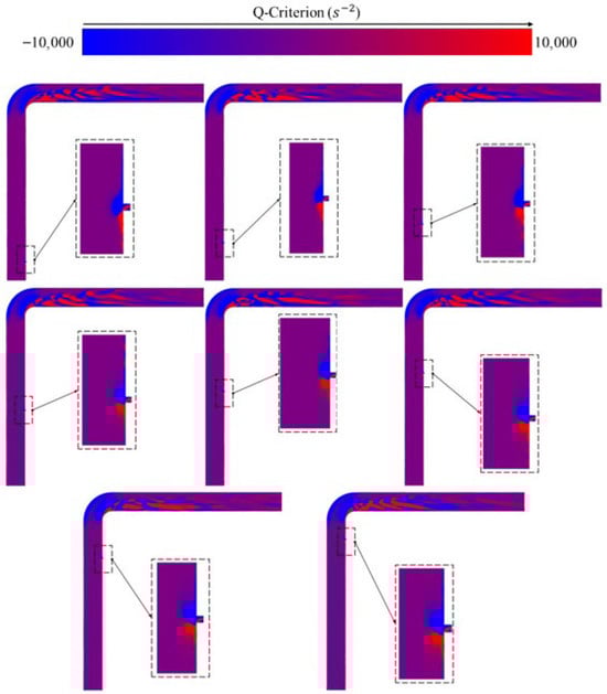
Figure 22.
Vortex distribution when leakage points are located at positions 1–8.
Figure 23 further analyzes the vortex distribution characteristics when leakage holes are located in the outlet section of the straight pipeline (positions 9–16). When the leakage holes are close to the bend exit (within a range of 100–400 mm from the exit), the vortex intensity at their locations significantly decreases, the vortex core diameter shrinks, and the vortex structures exhibit discrete distribution characteristics. This phenomenon indicates that the presence of leakage holes weakens the flow separation effect near the bend exit, altering the generation mechanism of vortex structures. Specifically, the leakage holes cause fluid mass loss at the bend exit, thereby reducing flow disturbances at the outlet end and disrupting the conditions required for vortex structure formation. Furthermore, the migration of the leakage hole locations significantly affects the vortex distribution downstream of the bend exit, with vortex intensity showing a nonlinear decay trend relative to the distance of the leakage holes from the exit. This phenomenon can be attributed to the gradual suppression of flow disturbances induced by the leakage holes during their propagation downstream of the bend exit due to viscous dissipation effects.
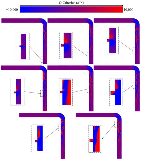
Figure 23.
Vortex distribution when leakage points are located at positions 9–16.
The evolution patterns of the velocity field and vortex distribution in the symmetrical plane of the bend are significantly influenced by the fluid properties and flow velocity. By selecting the position at the symmetrical plane, velocity contour maps are plotted, and the Q-criterion vortices with a threshold value of 0.06 are chosen to illustrate the distribution of vortices and velocity at the bend. The specific positions are depicted in Figure 24.
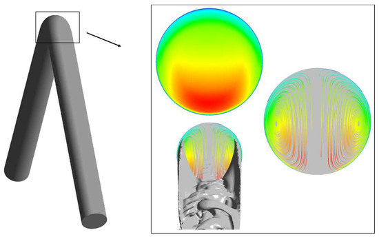
Figure 24.
Illustration of vortex and velocity distribution at the bend. The different colors represent the magnitude of velocity, with the scale being consistent with that of Figure 25.
Figure 25 illustrates the vortex and velocity distributions at the bend for the air medium under the inlet pressures of Air1, Air2, and Air3. Under Air1 conditions, as shown in Figure 25a, the flow velocity is significantly higher in the lower region, reaching up to 11 m/s. The relatively high-speed zone is close to the inner side of the bend, accounting for only about 20% of the area. The vortex structures are mainly distributed at the bottom and both sides of the bend. As shown in Figure 25b,c, under Air2 and Air3 conditions, the velocity contours are densely packed on the inner side of the bend, with local velocities exceeding 15 m/s. The high-speed areas account for approximately 30% and 50%, respectively, while the vortex structures remain concentrated at the bottom and both sides of the bend. The increase in flow velocity does not alter the distribution of vortices. The results also reveal significant spatial overlap between high-speed flow regions and high-vorticity regions. This is attributed to the centrifugal force on the inner side of the bend, which not only accelerates the fluid motion but also promotes vortex generation by enhancing the velocity gradient. Furthermore, the secondary flow structure on the inner side of the bend exhibits a clear left–right symmetrical distribution under the Q-criterion. The vortex core diameter is approximately 5 mm, and the vortex intensity increases as the bend curvature radius decreases. Near the bend exit, the complexity of the velocity contours is closely related to the distribution characteristics of the vortex structures. The increase in local velocity gradients directly corresponds to the enhancement of vortex intensity. This phenomenon validates the effectiveness of the Q-criterion in vortex identification, as it accurately captures the rotational motion characteristics in the flow through the second invariant of the velocity gradient tensor.
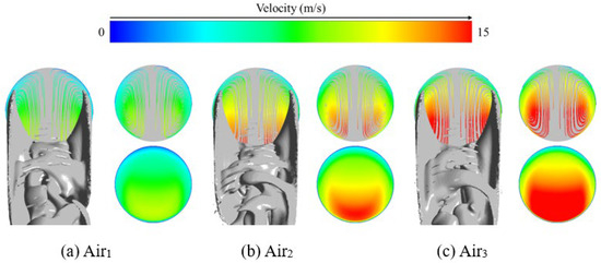
Figure 25.
Vortex and velocity distribution at the bend under different air flow velocities.
Figure 26 illustrates the vortex and velocity distribution characteristics in the bend region for the water medium under the inlet pressures of Water1, Water2, and Water3. In Figure 26a, the flow velocity in the lower region reaches up to 1 m/s, with high-speed areas concentrated on the inner side of the bend, accounting for approximately 10% of the region. The vortex structures are primarily distributed at the bottom and both sides of the bend. When the inlet pressure is adjusted to higher values, as shown in Figure 26b,c, the velocity gradient on the inner side of the bend significantly intensifies. In regions with dense velocity contours, the local flow velocity exceeds 3 m/s, and the proportion of high-speed areas reaches 20% and 50%, respectively.
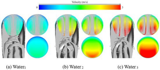
Figure 26.
Vortex and velocity distributions at the bend under different water flow velocities.
It is noteworthy that despite the increase in flow velocity, the vortex distribution pattern does not change. However, high-speed regions and high-vorticity regions exhibit significant spatial overlap. Compared to the air medium, the overall flow characteristics do not show significant changes, indicating that differences in fluid properties (such as viscosity and density) do not substantially alter the formation mechanism of secondary flow structures in the bend. Further analysis reveals that under the same geometric conditions, the water medium exhibits a more stable vortex core morphology, with vortex structure boundaries showing clearer continuity under the Q-criterion. In contrast, the vortex cores in the air medium are more diffuse, which may be attributed to the high viscosity of water suppressing small-scale turbulent disturbances.
During the progressive increase in inlet pressure, both media exhibit a positive correlation between vortex intensity and velocity gradient. However, the vorticity growth rate of the water medium is significantly lower than that of the air medium. This difference arises from the incompressibility of water, which limits drastic changes in the velocity field, while intermolecular forces enhance the uniformity of momentum transfer, thereby weakening the transverse shear effects driven by centrifugal forces.
4.3. Pressure Distribution Without Leakage Points
The pressure distribution characteristics inside a pipeline are crucial for evaluating system flow behavior and energy loss. As illustrated in Figure 27, which shows pressure contour distributions under different inlet pressures, the pressure field within the pipeline exhibits significant variations as the inlet pressure gradually increases. In the inlet section (the horizontal segment on the left side of the pipeline), the pressure contours generally display a uniform distribution trend due to the relatively stable inlet flow velocity, resulting in a small pressure gradient. In contrast, the pressure distribution in the pipeline bend and outlet section (the vertical segment below) shows distinct characteristics.
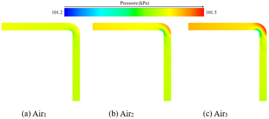
Figure 27.
Pressure distribution under different air flow velocities.
For the Air1 condition, as shown in Figure 27a, the pressure distribution is primarily around 101.4 kPa. The pressure gradient in the bend area is weak, and pressure changes are gradual, indicating minimal disturbance to the pressure field from flow separation and local resistance under low inlet pressure. As the inlet pressure increases to Air2, as depicted in Figure 27b, localized high-pressure regions appear near the larger bend, reaching up to 101.45 kPa. The peak pressure value increases, reflecting that higher inlet pressure leads to increased flow velocity, intensifying inertial effects and wall impact in the bend area, thereby enhancing local pressure loss and gradient variations.
When the inlet pressure reaches the Air3 condition, as shown in Figure 27c, the pressure near the larger bend exceeds 101.5 kPa. The high-pressure zone in the larger bend expands in both range and intensity, and the pressure contours in the outlet section become more chaotic. This indicates that under high inlet pressure, flow separation effects become significant, with energy loss concentrated in the bend and near-wall regions, further reducing the uniformity of the pressure distribution. Meanwhile, the pressure at the smaller bend consistently remains low, around 101.35 kPa.
From the perspective of pressure transmission characteristics, the increase in inlet pressure directly drives an overall elevation of the pressure level within the pipeline and expands the spatial influence range of pressure disturbances. The bend, as a key flow disturbance zone, exhibits a significantly enhanced pressure gradient with increasing inlet pressure, validating the fluid dynamics mechanism of “increased inlet pressure → higher flow velocity → inertial forces dominating the flow → intensified local resistance and pressure loss.” The morphology and distribution of pressure contours in the outlet section also indirectly reflect differences in flow outlet effects under varying inlet pressures, providing a visual basis for pressure field characteristics that can support subsequent modifications to pressure loss models and optimized flow design in pipeline systems.
As shown in Figure 28, under different inlet pressures ranging from Water1 to Water3, the pipeline pressure exhibits a gradual attenuation trend from the inlet to the outlet. In the inlet section, due to the coupling of the initial kinetic energy and pressure energy of the water flow, the pressure values remain close to the set inlet levels—approximately 101.45 kPa, 101.5 kPa, and 101.55 kPa, respectively. The pressure decreases with increasing distance from the inlet. When passing through the bend, the change in flow direction leads to localized resistance, resulting in significant variations in the pressure gradient. This creates a distribution pattern characterized by lower pressure on the inner side of the bend and relatively higher pressure on the outer side.
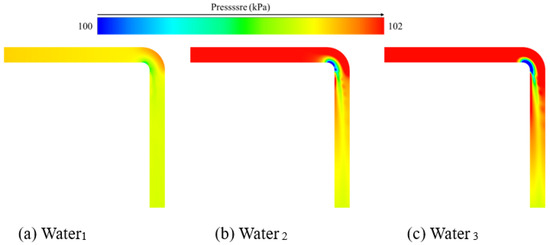
Figure 28.
Pressure distribution under different water flow velocities.
As the inlet pressure increases, the overall pressure level in the pipeline rises accordingly. The pressure in the inlet section grows linearly with the set inlet pressure, and the pressure difference across the bend also increases. Under the Water1 condition, the pressure distribution in the pipeline remains relatively smooth, with limited localized pressure disturbances near the bend. In the Water2 and Water3 conditions, higher inlet pressures enhance the kinetic energy of the water flow, intensifying flow separation and pressure redistribution effects at the bend. This leads to steeper gradients in the pressure contours. Although the attenuation rate of pressure in the outlet section follows a consistent pattern, the absolute pressure at the outlet increases with higher inlet pressure due to the transmission effect of elevated inlet pressure.
These observations indicate that the inlet pressure gradient directly regulates the overall energy level of the pipeline pressure field. Furthermore, in localized flow regions such as the bend, the intensity of pressure disturbances is positively correlated with the inlet pressure.
In summary, under different inlet pressures, the water pressure distribution inside the curved pipeline exhibits a decay trend from the inlet to the outlet, accompanied by localized pressure restructuring at the bend. As the inlet pressure gradient increases, the overall pressure level in the pipeline rises, and the local pressure difference at the larger bend expands, intensifying the gradient of the pressure contours. Meanwhile, the pressure at the smaller bend remains consistently low, which is attributed to the pronounced flow separation effect at this location.
4.4. Discussion
This study obtained the internal flow field characteristics of straight pipeline leakage during the transportation of different media through numerical calculations. In future work, the numerical calculation results of this study need to be further verified by experiments, which is a limitation of this study and also a direction for future work.
5. Conclusions
- (1)
- Regarding the fitting ability of the straight pipeline leakage location monitoring model, the nonlinear function models exhibit excellent prediction accuracy under the air medium (R2 > 0.99), while the fitting effect of the models under the water medium gradually weakens with the increase in inlet pressure (R2 decreases to 0.77 under Water3 condition), mainly limited by the damping effect of the liquid’s high viscosity on velocity field diffusion. Therefore, from a practical application perspective, under the air medium, there remains a one-to-one correspondence between the outlet flow velocity and the leakage hole location, allowing the leakage position to be reliably inferred directly from the outlet flow velocity. Under the water medium, it is necessary to control the inlet pressure below 1.04 × 10⁵ Pa (Water2 condition), while for high-pressure conditions, additional monitoring methods should be integrated to ensure positioning accuracy.
- (2)
- In terms of vorticity field evolution, the vorticity magnitude at the leakage hole under the air medium in the straight pipeline can reach more than 6 × 10⁵ s−2. In contrast, due to the high viscosity coefficient of the water medium, the vortex structures are rapidly dissipated, with a vorticity magnitude of only 1 × 10⁵ s−2 and showing asymmetric attenuation characteristics.
- (3)
- The migration of the leakage hole position leads to an increase in the density of local velocity contours. In a straight pipeline, the flow velocity in the central region is consistently higher than that in the edge region, and the flow velocity in the lower part of the edge region is significantly enhanced. The root cause can be attributed to the local pressure gradient disturbance and mass flux redistribution induced by the leakage hole.
- (4)
- For curved pipes, the analysis of pressure distribution characteristics reveals that an increase in the inlet pressure gradient directly elevates the overall pressure level within the pipeline and intensifies localized pressure disturbances in the bend region. In the air medium, the peak pressure at the larger bend under high inlet pressure increases significantly. In the water medium, the localized pressure restructuring effect in the curved pipe exhibits a linearly strengthening trend as the inlet pressure rises.
Author Contributions
Writing—review and editing, L.-H.T.; Investigation, Y.-F.Z.; Software, H.-F.H.; Conceptualization, Y.-J.Z.; Supervision, Writing-original draft, Y.-L.Z. All authors have read and agreed to the published version of the manuscript.
Funding
The research was financially supported by the Science and Technology Project of Quzhou (No. 2023NC08, 2022K41).
Data Availability Statement
The data presented in this study are available upon request from the corresponding author due to proprietary restrictions.
Conflicts of Interest
The authors declare no conflict of interest.
Nomenclature
| Symbol | Physical Meaning | Unit |
| k | Turbulent kinetic energy | m2/s2 |
| μt | Turbulent viscosity | Pa·s |
| σω | Turbulent Prandtl number | |
| Pk | Turbulent kinetic energy production term | Pa/s |
| β* | Model constant | |
| ω | Specific dissipation rate | 1/s |
| γ | Model coefficient | |
| β | Model constant | |
| F1 | Blending function | |
| R2 | Coefficient of determination | |
| Original efficiency data | ||
| Average value of the original efficiency data | ||
| Fitted data value |
References
- Lee, M.-R.; Lee, J.-H. A Study on Characteristics of Leak Signals of Pipeline Using Acoustic Emission Technique. Solid State Phenom. 2006, 110, 79–88. [Google Scholar] [CrossRef]
- Yao, L.; Zhang, L.; Wang, L.; Li, R.; Luo, H. A Spatiotemporal Data-Driven Framework for Acoustic Signal-Based Natural Gas Pipeline Leak Detection. IEEE Trans. Instrum. Meas. 2025, 74, 3527512. [Google Scholar] [CrossRef]
- Nguyen, D.-T.; Kim, J.-M. Trustworthy Pipeline Leak Localization Based on Acoustic Emission Event Monitoring. IEEE Trans. Instrum. Meas. 2025, 74, 3514311. [Google Scholar] [CrossRef]
- Saleem, F.; Ahmad, Z.; Kim, J.-M. Real-Time Pipeline Leak Detection: A Hybrid Deep Learning Approach Using Acoustic Emission Signals. Appl. Sci. 2025, 15, 185. [Google Scholar] [CrossRef]
- Yuan, Y.; Cui, X.; Han, X.; Gao, Y.; Lu, F.; Liu, X. Multi-condition pipeline leak diagnosis based on acoustic image fusion and whale-optimized evolutionary convolutional neural network. Eng. Appl. Artif. Intell. 2025, 153, 110886. [Google Scholar] [CrossRef]
- Duan, H.-F. Uncertainty Analysis of Transient Flow Modeling and Transient-Based Leak Detection in Elastic Water Pipeline Systems. Water Resour. Manag. 2015, 29, 5413–5427. [Google Scholar] [CrossRef]
- Adegboye, M.A.; Karnik, A.; Fung, W.-K. Numerical study of pipeline leak detection for gas-liquid stratified flow. J. Nat. Gas Sci. Eng. 2021, 94, 104054. [Google Scholar] [CrossRef]
- Roy, U. Leak Detection in Pipe Networks Using Hybrid ANN Method. Water Conserv. Sci. Eng. 2017, 2, 145–152. [Google Scholar] [CrossRef][Green Version]
- Rajasekaran, U.; Kothandaraman, M.; Pua, C.H. Water Pipeline Leak Detection and Localization With an Integrated AI Technique. IEEE Access 2025, 13, 2736–2745. [Google Scholar] [CrossRef]
- Behari, N.; Sheriff, M.Z.; Rahman, M.A.; Nounou, M.; Hassan, I.; Nounou, H. Chronic leak detection for single and multiphase flow: A critical review on onshore and offshore subsea and arctic conditions. J. Nat. Gas Sci. Eng. 2020, 81, 103460. [Google Scholar] [CrossRef]
- Al-Ammari, W.A.; Sleiti, A.K.; Rahman, M.A.; Rezaei-Gomari, S.; Hassan, I.; Hassan, R. Digital twin for leak detection and fault diagnostics in gas pipelines: A systematic review, model development, and case study. Alex. Eng. J. 2025, 123, 91–111. [Google Scholar] [CrossRef]
- Xie, J.; Xu, X.; Dubljevic, S. Long range pipeline leak detection and localization using discrete observer and support vector machine. AIChE J. 2019, 65, e16532. [Google Scholar] [CrossRef]
- Asada, Y.; Hagiwara, T.; Tsubota, T.; Kurasawa, T.S.K.; Kimura, M.; Azechi, I.; Iida, T. Field verification of single leak detection method based on transient pressures using optimization technique in in-situ irrigation pipeline system including branch junctions and diameter changes. Paddy Water Environ. 2025, 23, 243–262. [Google Scholar] [CrossRef]
- Delgado-Aguiñaga, J.A.; Besançon, G. EKF-based leak diagnosis schemes for pipeline networks. IFAC-PapersOnLine 2018, 51, 723–729. [Google Scholar] [CrossRef]
- Ahmad, S.; Ahmad, Z.; Kim, C.-H.; Kim, J.-M. A Method for Pipeline Leak Detection Based on Acoustic Imaging and Deep Learning. Sensors 2022, 22, 1562. [Google Scholar] [CrossRef]
- Cui, J.; Zhang, M.; Qu, X.; Zhang, J.; Chen, L. An Improved Identification Method of Pipeline Leak Using Acoustic Emission Signal. J. Mar. Sci. Eng. 2024, 12, 625. [Google Scholar] [CrossRef]
- Kam, S.I. Mechanistic modeling of pipeline leak detection at fixed inlet rate. J. Pet. Sci. Eng. 2010, 70, 145–156. [Google Scholar] [CrossRef]
- Li, W.; Fu, Q.; Gao, H. Pipeline leak detection and localization based on the flow balance and negative pressure wave methods. AIP Adv. 2024, 14, 115203. [Google Scholar] [CrossRef]
- Han, B.; Liu, X.; Liu, B.; Bao, H.; Jiang, X. Study on acoustic source characteristics of gas pipeline leakage. Noise Vib. Worldw. 2019, 50, 67–77. [Google Scholar] [CrossRef]
- Feng, Y.; Gao, J.; Yin, X.; Chen, J.; Wu, X. Risk assessment and simulation of gas pipeline leakage based on Markov chain theory. J. Loss Prev. Process Ind. 2024, 91, 105370. [Google Scholar] [CrossRef]
- Rui, Z.; Han, Q.; Zhang, H.; Wang, S.; Pu, H.; Ling, K. A new model to evaluate two leak points in a gas pipeline. J. Nat. Gas Sci. Eng. 2017, 46, 491–497. [Google Scholar] [CrossRef]
- Gao, Y.; Liu, Y.; Ma, Y.; Chen, X.; Yang, J. Application of the differentiation process into the correlation-based leak detection in urban pipeline networks. Mech. Syst. Signal Process. 2018, 112, 251–264. [Google Scholar] [CrossRef]
- Reda, A.; Mahmoud, R.M.A.; Shahin, M.A.; Amaechi, C.V.; Sultan, I.A. Roadmap for Recommended Guidelines of Leak Detection of Subsea Pipelines. J. Mar. Sci. Eng. 2024, 12, 675. [Google Scholar] [CrossRef]
- Vandrangi, S.K.; Lemma, T.A.; Mujtaba, S.M.; Ofei, T.N. Developments of leak detection, diagnostics, and prediction algorithms in multiphase flows. Chem. Eng. Sci. 2022, 248, 117205. [Google Scholar] [CrossRef]
- You, Y.; Seibold, F.; Wang, S.; Weigand, B.; Gross, U. URANS of turbulent flow and heat transfer in divergent swirl tubes using the k-ω SST turbulence model with curvature correction. Int. J. Heat Mass Transf. 2020, 159, 120088. [Google Scholar] [CrossRef]
- Di Piazza, I.; Ciofalo, M. Numerical prediction of turbulent flow and heat transfer in helically coiled pipes. Int. J. Therm. Sci. 2010, 49, 653–663. [Google Scholar] [CrossRef]
- Cabello, R.; Popescu, A.E.P.; Bonet-Ruiz, J.; Cantarell, D.C.; Llorens, J. Heat transfer in pipes with twisted tapes: CFD simulations and validation. Comput. Chem. Eng. 2022, 166, 107971. [Google Scholar] [CrossRef]
- Kato, Y.; Fujimoto, K.; Guo, G.; Kawaguchi, M.; Kamigaki, M.; Koutoku, M.; Hongou, H.; Yanagida, H.; Ogata, Y.Y.; Fujimoto, K.; et al. Heat transfer characteristics of turbulent flow in double-90-bend pipes. Energies 2023, 16, 7314. [Google Scholar] [CrossRef]
- Jinhee, J.; Hussain, F. On the identification of a vortex. J. Fluid Mech. 1995, 285, 69–94. [Google Scholar] [CrossRef]
- Liu, C.-Q.; Gao, Y.-S.; Dong, X.-R.; Liu, J.-M.; Zhang, Y.-N.; Cai, X.-S.; Gui, N. Third generation of vortex identification methods: Omega and Liutex/Rortex based systems. J. Hydrodyn. 2019, 31, 205–223. [Google Scholar] [CrossRef]


Disclaimer/Publisher’s Note: The statements, opinions and data contained in all publications are solely those of the individual author(s) and contributor(s) and not of MDPI and/or the editor(s). MDPI and/or the editor(s) disclaim responsibility for any injury to people or property resulting from any ideas, methods, instructions or products referred to in the content. |
© 2026 by the authors. Licensee MDPI, Basel, Switzerland. This article is an open access article distributed under the terms and conditions of the Creative Commons Attribution (CC BY) license.