Load Frequency Control via Multi-Agent Reinforcement Learning and Consistency Model for Diverse Demand-Side Flexible Resources

Abstract

With the high-proportion integration of renewable energy into the power grid, the fast-response capabilities of demand-side flexible resources (DSFRs), such as electric vehicles (EVs) and thermostatic loads, have become critical for frequency stability. However, the diverse dynamic characteristics of heterogeneous resources lead to high modeling complexity. Traditional reinforcement learning methods, which rely on neural networks to approximate value functions, often suffer from training instability and lack the effective quantification of resource regulation costs. To address these challenges, this paper proposes a multi-agent reinforcement learning frequency control method based on a Consistency Model (CM). This model incorporates power, energy, and first-order inertia characteristics to uniformly characterize the response delays and dynamic behaviors of EVs and air conditioners (ACs), providing a reduced-order analytical foundation for large-scale coordinated control. On this basis, a policy gradient controller is designed. By using projected gradient descent, it ensures that control actions satisfy physical boundaries. A reward function including state deviation penalties and regulation costs is constructed, dynamically adjusting penalty factors according to resource states to achieve priority configuration for frequency regulation. Simulations on the IEEE 39-node system demonstrate that the proposed method significantly outperforms traditional approaches in terms of frequency deviation, algorithm training efficiency, and frequency regulation economy.

1. Introduction

The large-scale integration of renewable energy and the electrification of the demand side are driving the power system toward a rapid transition to a high-proportion renewable energy and high-proportion power electronic device paradigm. Power electronic devices, relying on semiconductor-based converter technology, cannot provide the mechanical inertia support inherent in traditional synchronous generators [1]. Meanwhile, the significant decline in the penetration rate of traditional synchronous generators further exacerbates the attenuation of the system’s overall inertia level [2,3]. The large-scale integration of intermittent renewable energy sources (RESs), such as wind and photovoltaic (PV) power, has intensified power fluctuations in electrical grids, posing significant challenges to frequency stability [4,5]. Although traditional generation-side regulation remains indispensable, DSFRs, including EVs and thermostatically controlled loads, have become an important complement to frequency regulation due to their controllability and fast-response capabilities.

In recent years, growing global interest in DSFRs has been witnessed. However, the capacity limitations and diversity of individual units make it impossible for them to participate in frequency modulation (FM) directly, so resource aggregation and quantification have become key to unlocking their FM potential [6,7]. For instance, reference [8] explored the role of EVs in peak shaving and frequency regulation from the perspective of vehicle/grid interaction. References [9,10] used Markov state models to aggregate load populations. Reference [11] developed an equivalent energy storage model for ACs by discretizing load power regulation. Such studies provide a theoretical basis for the improvement in frequency deviation using a single type of DSFR. Reference [12] proposed an optimized method for the frequency response by constructing a dynamic model of the AC system and integrating EV scheduling strategies. Reference [13] investigated the role of EVs and energy storage devices in islanded hybrid microgrids for frequency regulation and proposed a variety of advanced control strategies that can effectively improve the frequency stability of the system. Reference [14] proposed that the aggregator must master the flexibility of clustering and analytically represent the aggregated feasible domain of the power curve. References [15,16] adopted high-dimensional multivariate load aggregation models to reflect real-time energy dynamics. However, these methods focus on detailed state parameters and suffer from high complexity; moreover, the number of parameters grows exponentially with the order, leading to difficulties in model convergence during real-time control and limiting their applicability in large-scale coordinated scenarios.

Traditional frequency control methods, which rely on physical models to construct control strategies and leverage the advantages of simple parameter tuning and clear response mechanisms, have long supported the frequency stability of power systems. Reference [17] proposed a multistage constant compressor speed control strategy based on genetic algorithms, setting temperature as the input control factor and compressor speed as the output factor to optimize the control strategy. Reference [18] developed a novel PID control scheme for the Pound/Drever/Hall frequency tracking system, aiming to address the instability of theoretical inputs and the difficulty in accurately determining the transfer functions of controlled modules and actuators. Reference [19] introduced a consensus strategy derived from droop control, enabling distributed battery energy storage systems to simultaneously participate in different frequency control requirements. However, these methods are highly dependent on precise system parameters and fixed operational scenario assumptions, exposing significant limitations in complex environments with high-proportion new energy grid integration and diverse DSFR participation: On one hand, the output fluctuations of intermittent power sources such as wind and PV exhibit strong randomness, while the dynamic responses of DSFRs show nonlinear and time-varying characteristics. Traditional models struggle to accurately characterize the complex coupling relationships among multiple agents. On the other hand, fixed control parameters cannot adaptively adjust to match the real-time changing potential of frequency regulation resources, leading to decreased control accuracy and imbalance in the system economy.

The participation of diverse flexible resources in frequency response control within power systems involves massive and complex data, which are not only large-scale and high-dimensional but also difficult to acquire. Traditional methods have strict requirements for data integrity and accuracy, and their control effectiveness in frequency response is compromised when data are incomplete or exhibit complex nonlinear relationships [20,21]. Deep Reinforcement Learning (DRL) can automatically learn highly abstract and effective feature representations from massive, complex, or even incomplete data, and solve for optimal frequency control strategies under difficult data acquisition conditions by continuously exploring different flexible resource control schemes [22]. Reference [23] proposed a DRL-based control strategy to minimize the energy consumption of heating, ventilation, and air conditioning (HVAC) systems and user thermal discomfort. Reference [24] developed a novel Deep Q-Network (DQN) algorithm with tilt-based fuzzy cascade control for system frequency regulation across different operating regions. Reference [25] introduced a large-scale multi-agent twin delayed Deep Deterministic Policy Gradient (DDPG) algorithm with congenital cognition for load frequency control (LFC), incorporating prior knowledge into agents before pre-training based on human innate cognitive mechanisms. However, these methods consider the long-term costs of constraints through expected values but cannot guarantee constraint satisfaction at every time step. Reference [26] proposed a DDPG-based dynamic droop control strategy to determine optimal droop gains via a multi-reward function design for real-time optimal operation and frequency regulation. Reference [22] developed a simulator network with a historical database instead of a critic network to obtain policy gradients for backpropagation. Nonetheless, these approaches overlook the security risks of constraint violations caused by poorly trained reinforcement learning (RL) policies during training [27]. Specifically, without model knowledge, RL policies learn from the feedback of random exploration (i.e., trial-and-error), where random control decisions may frequently violate system operation constraints. Agents in traditional online DRL methods require extensive “trial-and-error,” leading to erroneous decisions [28]. Such erroneous decisions can result in uncomfortable indoor temperatures in buildings and suboptimal regulation performance, imposing high costs in practice and rendering them unreliable for power systems demanding high operational reliability.

To address the above challenges, this paper proposes a multi-agent reinforcement learning method based on a CM to fully leverage the speed and flexibility of demand-side resources in frequency control. First, a coordinated control model for different types of flexible resources participating in grid frequency regulation is established. By utilizing the analytical tractability of reduced-order models, transfer functions for integrating the frequency regulation process are developed to match the required dynamic frequency response. Subsequently, abandoning the DDPG’s reliance on neural networks to approximate value functions, an analytical controller based on frequency deviation gradients is designed. A reward function incorporating the regulation cost of flexible resources is constructed, integrating the state of charge of EVs and temperature deviation penalties for ACs, thereby optimizing the participation of flexible resources. The contributions of this study to the research field are as follows:

• A universal model incorporating power constraints, energy constraints, and first-order inertia characteristics is constructed, using only a few key parameters to characterize resource response delays and dynamic behaviors.
• A policy gradient controller is designed to guide the update of agent network parameters by combining frequency deviations and resource response characteristics. Through projected gradient descent, the parameter update direction is adjusted to the tangent direction of the feasible domain, ensuring that actions always satisfy constraints.
• A novel reward function for frequency control is proposed, dynamically adjusting weight factors and penalty terms based on resource states to achieve a priority configuration for different optimization objectives.

This paper is organized as follows. Section 2 proposes a model that unifies the state parameters to describe the response characteristics of different types of flexibility resources. Section 3 demonstrates the parameter updating mechanism to improve the DDPG algorithm with the participation of demand-side resources. Section 4 verifies the effectiveness of the proposed method by a 39-node system.

2. A Consistency Model for Frequency Control Involving Diverse Flexible Resources

The large geographic distribution, tiny individual size, and variety of types of flexible resources allow for quick reactions to changes in system frequency. However, there are several obstacles to overcome when modeling numerous resources in depth: The addition of more state variables makes the regulation process more difficult and drastically increases the model order. Given that a uniform first-order lag element can be used to represent EVs and ACs in standardized modeling during grid frequency control, this paper proposes a unified characterization of dynamic features based on their shared properties. This approach achieves substantial model simplification while preserving essential physical features.

2.1. Consistency Model for Air Conditioning Loads

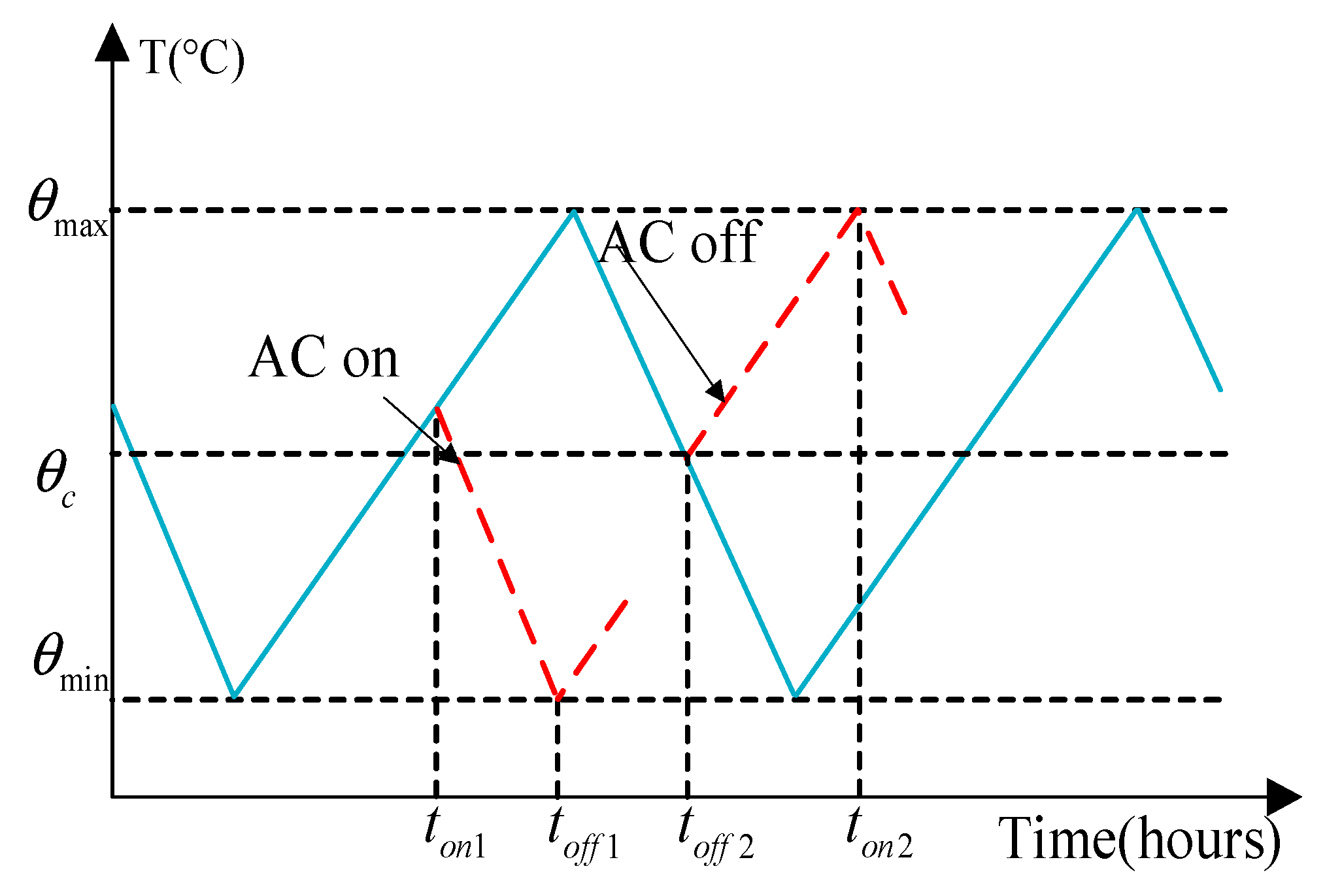
The activation/deactivation of AC units depends on whether the indoor temperature resides within a predefined setpoint range. The interior temperature must be kept within higher and lower bounds, as seen in Figure 1. The ACs automatically turn on when the temperature rises over the upper threshold and turn off when it falls below the lower threshold. Within the permissible temperature range, AC units exhibit dual-frequency regulation capabilities: They can be activated to give a downward regulating capacity as long as the indoor temperature is within acceptable limitations and the AC is turned off. On the other hand, the ACs can be turned off to provide an upward regulation capacity if the interior temperature remains within acceptable limits.

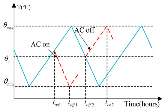
Figure 1. Air-conditioning load operation characteristic diagram.

The first-order thermodynamic equivalent model for ACs’ differential equation is written as follows:

$${\theta }_i^{t+1}={\theta }_i^t+\alpha ({\theta }_0^t-{\theta }_i^t)-b{P}_{\mathrm{AC}}^{\max }{s}_t$$

(1)

where $\alpha$ is the thermal inertia coefficient, $\alpha =1/RC$; $R$ represents the building’s equivalent thermal resistance; $C$ denotes the equivalent thermal capacitance; $b=\eta /C$; $\eta$ is the energy efficiency coefficient; $P_{\mathrm{AC}}^{\max }$ is the AC’s power consumption; ${\theta }_0^t$ is the ambient temperature; ${\theta }_i^t$ is the interior temperature; and $s_t$ is the binary on/off state. The interior temperature equation during period V is as follows:

$${\theta }_V={(1-\alpha )}^V{\theta }_0+\alpha {\displaystyle \sum _{t=1}^V{(1-\alpha )}^V}{\theta }_i-b{\displaystyle \sum _{t=1}^V{(1-\alpha )}^{V-t}}{P}_{\mathrm{AC}}^{\max }{s}_t$$

(2)

The temperature limitations are as follows in order to avoid frequent switching brought on by temperature dead bands:

$${\theta }_c-{\displaystyle \frac{\epsilon }{2}}\le {\theta }_i\le {\theta }_c+{\displaystyle \frac{\epsilon }{2}}$$

(3)

where ${\theta }_c$ is the AC’s setpoint temperature and $\epsilon$ is the dead band width. Combining Equations (2) and (3) yields the following:

$$-{\displaystyle \frac{{\theta }_c+\frac{\epsilon }{2}-{\theta }_V}{b}}\le {\displaystyle \sum _{t=1}^V{(1-\alpha )}^{V-t}}{P}_{\mathrm{AC}}^{\max }{s}_t\le -{\displaystyle \frac{{\theta }_c-\frac{\epsilon }{2}-{\theta }_V}{b}}$$

(4)

While the AC’s electrical power consumption and interior temperature are generally constant during steady-state operation, changes to the AC’s setpoint temperature upset the indoor thermal equilibrium. However, a shift from steady-state to dynamic behavior is triggered by a change in the setpoint temperature. The ACs’ electrical power reacts instantly during this brief period, while the building’s thermal inertia causes the indoor temperature to fluctuate slowly. This lag persists until a new thermal equilibrium is established, restoring the system to steady-state conditions.

The discrete power variable $P_{\mathrm{AC}}^{\max }{s}_t$ is converted to a continuous variable $P^{\mathrm{AC}}$, with the constraint expressed as follows [29]:

$$0\le P^{\mathrm{AC}}\le P_{\mathrm{AC}}^{\max }$$

(5)

The ACs’ energy is completely used up when the room temperature hits the top limit, as shown by the adjustable power capacitance being zero. In contrast, the energy of the ACs is fully charged when the room temperature falls to the lower limit. The baseline charging/discharging power for the ACs cluster is defined as follows [30]:

$$P_t^{\mathrm{base}}={\displaystyle \frac{{\theta }_0-{\theta }_c}{\eta R}}$$

(6)

where $P_t^{\mathrm{base}}$ is the baseline charging/discharging power of the AC cluster.

$$S_{t+1}^{\mathrm{AC}}=(1-\alpha )S_t^{\mathrm{AC}}+(P_t^{\mathrm{AC}}-P_t^{\mathrm{base}})\Delta t$$

(7)

where $S_t^{AC}$ is the energy state of ACs at time t; $S_{t+1}^{AC}$ is the energy state of ACs at time t + 1; and $\Delta t$ is the time step duration.

The upper and lower limits of the CM’s charging/discharging power can be obtained:

$$P_t^{\mathrm{ACmax}}=P_t^{\mathrm{ACsummax}}-P_t^{\mathrm{base}}$$

(8)

$$P_t^{\mathrm{ACmin}}=P_t^{\mathrm{ACsummin}}-P_t^{\mathrm{base}}$$

(9)

where $P_t^{\mathrm{ACsummax}}$ and $P_t^{\mathrm{ACsummin}}$ are the maximum and minimum power limits of the ACs cluster, respectively.

The aggregated ACs cluster CM is expressed as follows:

$$P_t^{\mathrm{ACmin}}\le P_t^{\mathrm{AC},\mathrm{CM}}\le P_t^{\mathrm{ACmax}}$$

(10)

$$S_t^{\mathrm{ACmin}}\le S_t^{\mathrm{AC},\mathrm{CM}}\le S_t^{\mathrm{ACmax}}$$

(11)

$$S_t^{\mathrm{AC},\mathrm{CM}}=(1-\alpha )S_t^{\mathrm{AC},\mathrm{CM}}+P_t^{\mathrm{AC},\mathrm{CM}}\Delta t$$

(12)

where $S_t^{\mathrm{AC},\mathrm{CM}}$ and $P_t^{\mathrm{AC},\mathrm{CM}}$ represent the energy state and power of the ACs cluster CM, respectively; $P_t^{\mathrm{ACmax}}$ and $P_t^{\mathrm{ACmin}}$ denote its upper and lower power limits; and $S_t^{\mathrm{ACmax}}$ and $S_t^{\mathrm{ACmin}}$ indicate its maximum and minimum energy state boundaries.

The transfer function of the aggregated ACs cluster, which participates in frequency regulation, can be mathematically represented. Consequently, the following link between frequency deviation and power output is obtained by this paper’s derivation of the equivalent transfer function for the ACs cluster CM involved in frequency regulation:

$$\Delta P_{\mathrm{AC}}(s)={\displaystyle \frac{K_{\mathrm{AC}}}{1+T_{\mathrm{AC}}s}}{e}^{-{\tau }_{\mathrm{AC}}s}\Delta f(s)$$

(13)

where $\Delta P_{\mathrm{AC}}(s)$ is the charging/discharging power of the ACs cluster to the grid; $T_{\mathrm{AC}}$ is the charge/discharge time constant of the ACs cluster; $K_{\mathrm{AC}}$ is the droop control parameter of the ACs cluster; ${\tau }_{\mathrm{AC}}$ is the time delay of ACs; and $s$ is the Laplace variable.

When flexible resources are in a high state of charge, their charge/discharge efficiency is higher, and they should be prioritized for charge/discharge operations. Therefore, the relationship between the state of charge of flexible resources and the droop control coefficient is as follows:

$$K_{\mathrm{FL}}=K_{\mathrm{FLbase}}(1-{\displaystyle \frac{|F_{\mathrm{SOC}}^{\mathrm{FL}}-F_{\mathrm{SOCS}}^{\mathrm{FL}}|}{F_{\mathrm{SOCS}}^{\mathrm{FL}}}})$$

(14)

where $K_{\mathrm{ACbase}},K_{\mathrm{EVbase}}\in K_{\mathrm{FLbase}}$, $K_{\mathrm{ACbase}}$, and $K_{\mathrm{EVbase}}$ are the reference droop control coefficients for ACs and EVs, respectively; $F_{\mathrm{SOCS}}^{\mathrm{FL}}$ is the set value of the state of charge of flexible resources; $F_{\mathrm{SOC}}^{\mathrm{FL}}$ is the state of charge of flexible resources; and $K_{\mathrm{FLbase}}$ is the reference droop control coefficient of flexible resources.

2.2. Consistency Model for Electric Vehicles

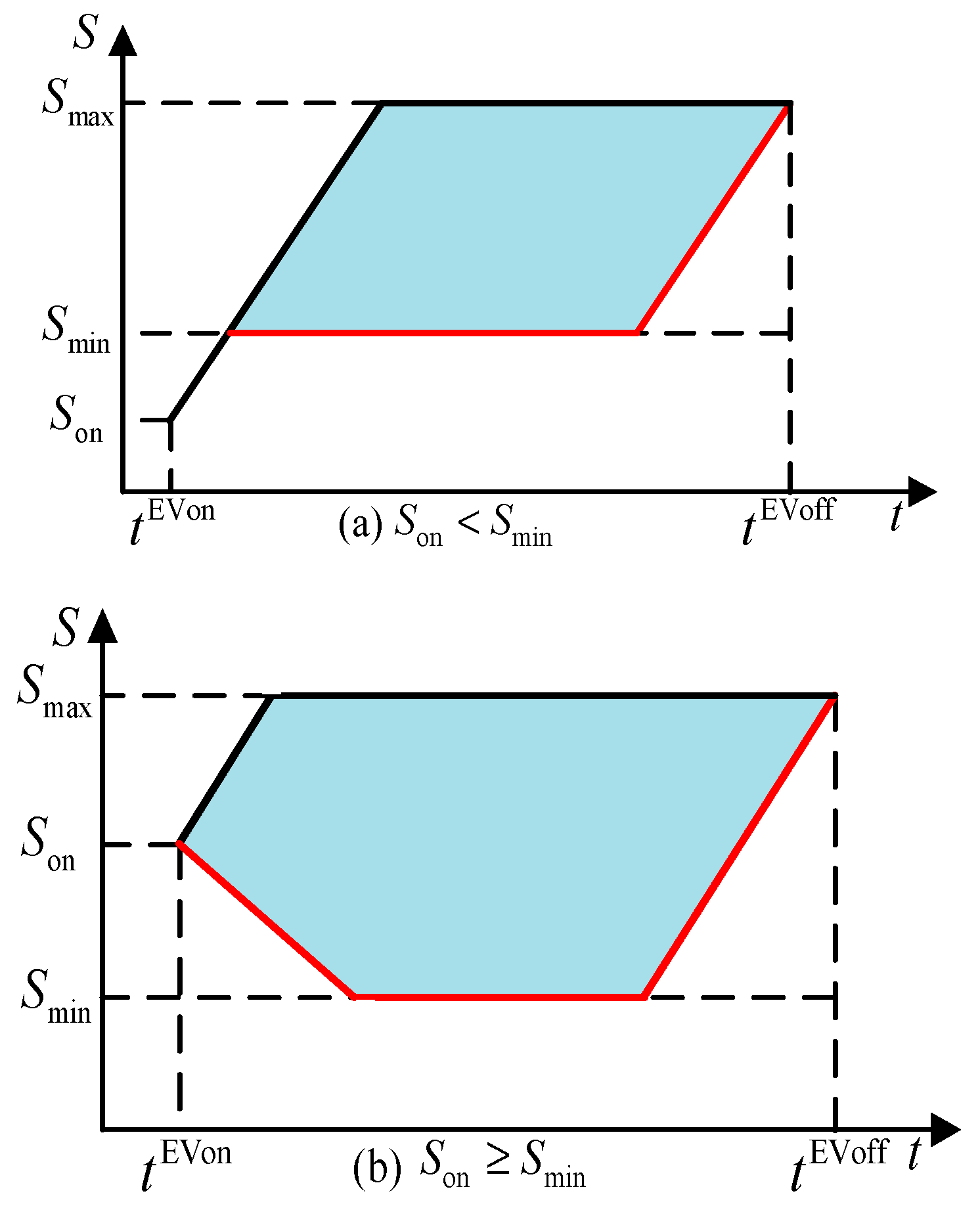
Users’ desire to participate in peak-shaving auxiliary services, such as virtual energy storage, is crucial, because EV owners have the option to discontinue the service at any moment. Such opt-out behavior affects control tactics by creating uncertainty during the planned service period. The viable charging/discharging power zone in Figure 2 that takes into account EV user behavior is shown by the shaded area. The frequency regulation capability of EVs exhibits strong coupling with user behavior characteristics. Therefore, it is necessary to construct a model that integrates the following:

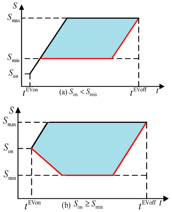
Figure 2. Feasible range of electric vehicle charging and discharging.

In the figure, the red line segment represents the lower bound of the feasible charging/discharging region for EVs, indicating the minimum battery energy requirement during regulation. Here, $t^{\mathrm{EVon}}$ denotes the grid-connection time of EVs, and $t^{\mathrm{EVoff}}$ represents the grid-disconnection time.

The energy feasible region in Figure 2a is determined by Equations (15) and (16), while that in Figure 2b is defined by Equations (15)–(18). The upper and lower power limits derived from these energy feasible regions are given by Equations (19) and (20), respectively.

$$S_i^{\mathrm{EVmax}}(t)=\min \left\{(S_i^{\mathrm{on}}+P_i^{\max }\left(t-t_i^{\mathrm{EVon}}\right),S_i^{\max }\right\}t\in [t_i^{\mathrm{EVon}},t_i^{\mathrm{EVoff}}]$$

(15)

$$S_i^{{\mathrm{EVmin}}^{\prime }}(t)=\max \left\{(S_i^{\mathrm{on}}+P_i^{\min }\left(t-t_i^{\mathrm{EVon}}\right),S_i^{\min }\right\}t\in [t_i^{\mathrm{EVon}},t_i^{\mathrm{EVoff}}]$$

(16)

$$S_i^{{\mathrm{EVmin}}^{″}}(t)=\max \left\{(S_i^{\mathrm{ex}}+P_i^{\min }\left(t_i^{\mathrm{EVoff}}-t\right),S_i^{\min }\right\}t\in [t_i^{\mathrm{EVon}},t_i^{\mathrm{EVoff}}]$$

(17)

$$S_i^{\mathrm{EVmin}}(t)=\max \{(S_i^{{\mathrm{EVmin}}^{\prime }}(t),S_i^{{\mathrm{EVmin}}^{″}}(t)\}t\in [t_i^{\mathrm{EVon}},t_i^{\mathrm{EVoff}}]$$

(18)

$$P_i^{\mathrm{EVmax}}(t)=\min \left\{{\displaystyle \frac{S_i^{\mathrm{EVmax}}(t+1)-S_i^{\mathrm{EVmax}}(t)}{\Delta t}},P_i^{\max }\right\}$$

(19)

$$P_i^{\mathrm{EVmin}}(t)=\max \left\{{\displaystyle \frac{S_i^{\mathrm{EVmax}}(t+1)-S_i^{\mathrm{EVmax}}(t)}{\Delta t}},P_i^{\min }\right\}$$

(20)

where $S_i^{\mathrm{EVmax}}(t)$ and $S_i^{\mathrm{EVmin}}(t)$ are the maximum and minimum energy states of the EVs at time t; $P_i^{\mathrm{EVmax}}(t)$ and $P_i^{\mathrm{EV}\min }(t)$ represent the maximum charging and discharging power of the i-th EVs; $S_i^{{\mathrm{EVmin}}^{\prime }}(t)$ and $S_i^{{\mathrm{EVmin}}^{″}}(t)$ denote the minimum energy thresholds at grid-connection and disconnection times; $S_i^{\mathrm{on}}$ is the initial energy state of the i-th EVs when connecting to the grid; $S_i^{\mathrm{ex}}$ is the required energy state of the i-th EVs when disconnecting from the grid; $t_i^{\mathrm{EVon}}$ and $t_i^{\mathrm{EVoff}}$ indicate the grid-connection and disconnection times of the i-th EVs; and $\Delta t$ is the period.

The EVs unit’s power and electricity boundaries can be used to determine the EV cluster’s boundary in the manner described below [31]:

$$S_t^{\mathrm{EV},\mathrm{CMmax}/\min }={\displaystyle \sum _{i=1}^{N_{\mathrm{EV}}}{S}_i^{\mathrm{EVmax}/\min }}{x}_i(t)$$

(21)

$$P_t^{\mathrm{EV},\mathrm{CMmax}/\min }={\displaystyle \sum _{i=1}^{N_{\mathrm{EV}}}{P}_i^{\mathrm{EVmax}/\min }}{x}_i(t)$$

(22)

where $N_{\mathrm{EV}}$ is the number of EV clusters; $x_i(t)$ represents the grid-connected status of the i-th vehicle; $S_i^{\mathrm{EVmax}/\min }$ are the upper and lower limits of the electrical energy of the EV cluster CM; $P_i^{\mathrm{EVmax}/\min }$ are the upper and lower limits of the power of the EV cluster CM.

The EV cluster CM is as follows:

$$P_t^{\mathrm{EV},\mathrm{CM}\min }\le P_t^{\mathrm{EV},\mathrm{CM}}\le P_t^{\mathrm{EV},\mathrm{CMmax}}$$

(23)

$$S_t^{\mathrm{EV},\mathrm{CM}\min }\le S_t^{\mathrm{EV},\mathrm{CM}}\le S_t^{\mathrm{EV},\mathrm{CMmax}}$$

(24)

$$S_t^{\mathrm{EV},\mathrm{CM}}=S_t^{\mathrm{EV},\mathrm{CM}}+P_t^{\mathrm{EV},\mathrm{CM}}\Delta t$$

(25)

where $S_t^{\mathrm{EV},\mathrm{CM}}$ and $P_t^{\mathrm{EV},\mathrm{CM}}$ are the energy state and power of the EV cluster’s CM, respectively.

The EV cluster CM involved in frequency regulation has the following comparable transfer function:

$$\Delta P_{\mathrm{EV}}(s)={\displaystyle \frac{K_{\mathrm{EV}}}{1+T_{\mathrm{EV}}s}}{e}^{-{\tau }_{\mathrm{EV}}s}\Delta f(s)$$

(26)

where $\Delta P_{\mathrm{EV}}(s)$ is the charging/discharging power of the EV cluster to the grid; $T_{\mathrm{EV}}$ is the charge/discharge time constant of the EV cluster; $K_{\mathrm{EV}}$ is the droop control parameter of the EV cluster; and ${\tau }_{\mathrm{EV}}$ is the time delay of EVs.

2.3. Assessing the Controllable Potential Considering the Uncertainty of Flexible Resources

In the above-mentioned CM for flexible resources, the number of flexible resources connected to the power grid at any given time is highly correlated with the maximum and minimum charging and discharging power, as well as the upper and lower limits of the electricity quantity. To meet the time margin mandated by the power market regulations at the day-ahead stage, a system for predicting parameters must be established based on historical data and user behavior patterns. By mining the spatiotemporal distribution patterns of the operating status of flexible resource clusters, we can predict the time-series changes in the number of resource accesses in each period, allowing for the daily calculation of the power and electricity boundaries of the CM response capability.

The boundary parameters of power and electricity in the CM are predicted using the gate-controlled cyclic unit technique, which has high processing capabilities for time-series data. The historical data of CM’s initial state of charge, grid-connection time, and off-grid time are separated into training and testing groups for the day-ahead prediction stage, which is based on the gate-controlled cyclic unit algorithm. The training group’s historical data are then used to mine the data’s inherent connections. Rolling correction mainly includes three situations: new flexible resources connected to the grid during the response period, flexible resources delayed off-grid, and early off-grid.

• For flexible resources newly connected to the grid during the response period, if the demand-side flexible resources can reach the minimum power capacity at the end of the response period, the lower limit of the FM power potential of the flexible resources will be corrected:

$$F_{\Delta \mathrm{SOC},k}^{\mathrm{CM}\min }=F_{\mathrm{SOC},\mathrm{CM}}^{\mathrm{targe}\mathrm{t}}-{\displaystyle \frac{P_{\mathrm{CM}}^{\max }{\eta }_c[t_{\mathrm{CM}}^{\mathrm{set}}-(k\Delta t+T)]}{S_{\mathrm{CM}}}}$$

(27)

$$P_t^{\mathrm{CMmin}}=\left\{\begin{array}{l}\min (P_{\mathrm{CM}}^{\max },{\displaystyle \frac{F_{\Delta \mathrm{SOC},k}^{\mathrm{CM}\min }{S}_{\mathrm{CM}}}{{\eta }_c(k\Delta t+T-t_0)}}),F_{\Delta \mathrm{SOC},k}^{\mathrm{CM}\min }\ge 0\\ \max (P_{\mathrm{CM}}^{\min },{\displaystyle \frac{F_{\Delta \mathrm{SOC},k}^{\mathrm{CM}\min }{S}_{\mathrm{CM}}}{{\eta }_d(k\Delta t+T-t_0)}}),F_{\Delta \mathrm{SOC},k}^{\mathrm{CM}\min }<0\end{array}\right.$$

(28)

where $t_0$ is the current moment; $k\Delta t+T$ is the moment when the response ends; $F_{\Delta \mathrm{SOC},k}^{\mathrm{CM}\min }$ is the minimum charging amount or the maximum discharging amount of the flexible resource; $S_{\mathrm{CM}}$ is the electrical energy of the flexible resource; ${\eta }_c$ and ${\eta }_d$ are the charging and discharging efficiencies, respectively; $F_{\mathrm{SOC},\mathrm{CM}}^{\mathrm{targe}\mathrm{t}}$ is the set value of the state of charge when the flexible resource is off-grid; $t_{\mathrm{CM}}^{\mathrm{set}}$ is the set off-grid moment; $P_{\mathrm{CM}}^{\max }$ is the maximum charging and discharging power; and $P_t^{\mathrm{CM}\min }$ is the lower limit of the frequency regulation power within the response period.

The upper limit of the FM power potential needs to be revised to prevent flexible resources from overcharging during the response period:

$$P_t^{\mathrm{CMmax}}=\min (P_{\mathrm{CM}}^{\max },{\displaystyle \frac{F_{\Delta \mathrm{SOC},k}^{\mathrm{CM}\max }{S}_{\mathrm{CM}}}{{\eta }_c\cdot (k\Delta t+T-t_0)}})$$

(29)

$$F_{\Delta \mathrm{SOC},k}^{\mathrm{CM}\max }=100\%-F_{\mathrm{SOC}}^{\mathrm{CM}}(t_0)$$

(30)

where $F_{\Delta \mathrm{SOC},k}^{\mathrm{CM}\max }$ is the allowable increase in the electrical energy of the flexible resource within the remaining time of the response period; $P_t^{\mathrm{CMmax}}$ is the upper limit of the frequency regulation power within the response period; and $F_{\mathrm{SOC}}^{\mathrm{CM}}(t_0)$ is the state of charge of the flexibility resource at time $t_0$.

2.

Similar to the earlier addressed scenario for the recently grid-connected flexible resources, the frequency regulation capability of the remaining period should be re-evaluated for flexible resources with a delayed off-grid time if the CM has reached the set electrical energy. If the CM has not reached the set electrical energy, the upper and lower limits of the frequency regulation power of the flexible resources should be revised to the allowable maximum charging power.

3.

For the flexible resources that go off-grid in advance, the upper and lower limits of their frequency regulation power should be revised to zero, and they will not participate in the frequency response for the remaining time.

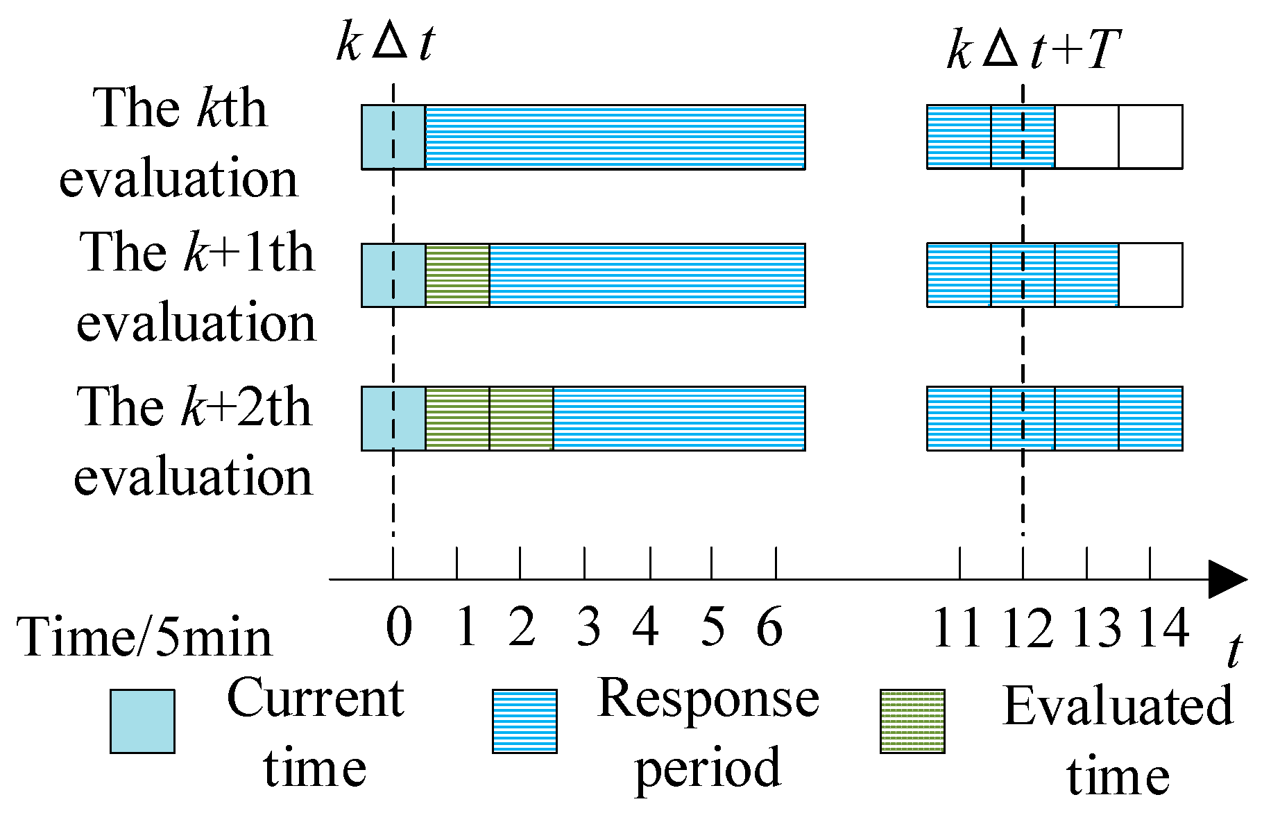
The rolling correction and evaluation process of the frequency regulation potential is shown in Figure 3. Among them, $\Delta t$ is the evaluation time interval; $T$ is the length of the evaluation period; and $\Delta t$ and $T$ are set to 5 min and 1 h, respectively.

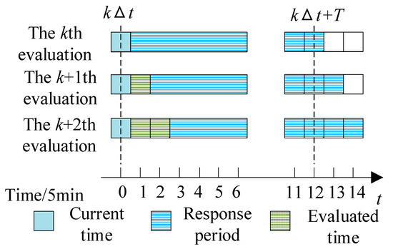
Figure 3. Rolling evaluation diagram of flexible resource frequency modulation potential.

2.4. Consistency Model Considering the Participation of Different Types of Resources in Frequency Control

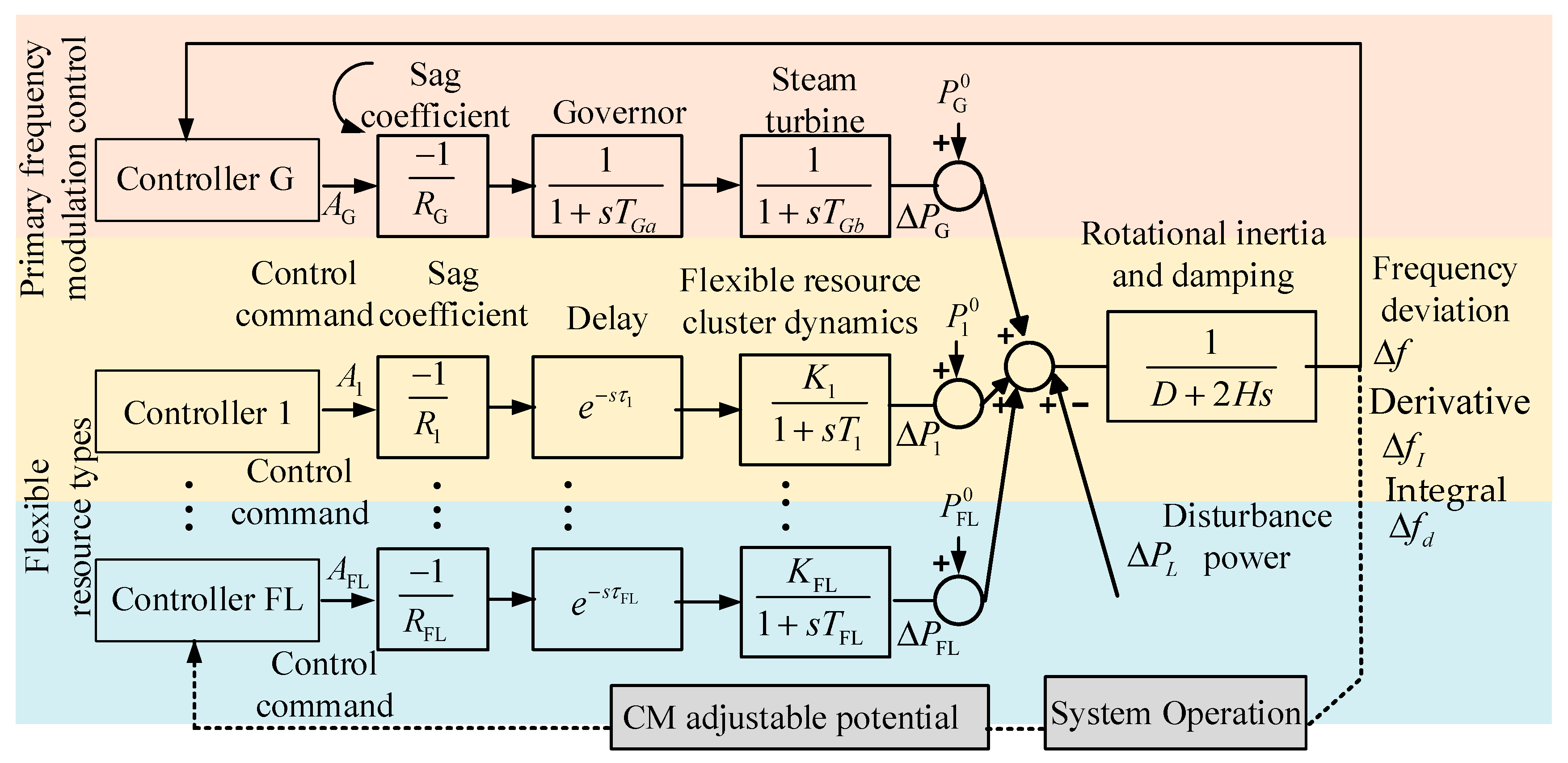
Agents are used to control large-scale, variable resources. Figure 4 illustrates how the power grid frequency control model is set up with flexible resources involved. Among them, $R_{\mathrm{G}}$, $R_1$, and $R_{\mathrm{FL}}$ are the sag control coefficients; $T_{\mathrm{Ga}}$ and $T_{\mathrm{Gb}}$ are the time constants of the speed governor of the frequency regulation unit and the steam turbine unit, respectively; $K_1$, $T_1$, $e^{-s{\tau }_1}$, $K_{\mathrm{FL}}$, $T_{\mathrm{FL}}$, and $e^{-s{\tau }_{\mathrm{FL}}}$ represent the sag control parameters, the time constant, and the time delay link of the different flexible resource cluster, respectively; ${\tau }_1$ and ${\tau }_{\mathrm{FL}}$ represent the delay time constant of the different flexible resource cluster; $\Delta P_1$ and $\Delta P_{\mathrm{FL}}$ represent the power output of different flexibility resources, respectively; $\Delta P_{\mathrm{G}}$ denotes the generator power output; $\Delta P_L$ is the disturbance power; and $s$ is the Laplace-transform variable. The inputs of the controller include the system frequency deviation $\Delta f$, the derivative $\Delta f_I$ and the integral $\Delta f_d$ of the deviation, the reference operating points $P_{\mathrm{FL}}^0$, $P_1^0$, and $P_{\mathrm{G}}^0$ of the flexible resource and generator unit, and the adjustable potential of the CM. $H$ and $D$ are the system inertia time constant and load damping coefficient. Their output is the control command $A_{\mathrm{G}}$, $A_1$, and $A_{\mathrm{FL}}$ of each frequency regulation unit. The frequency regulation unit’s power adjustment amount is determined by the controller’s output and the droop control coefficient. The power variation of the flexible resources in the frequency response can be expressed as follows:

$$\Delta P_{\mathrm{FL},j}=A_j-{\displaystyle \frac{\Delta f}{R_j}}$$

(31)

where $\Delta P_{\mathrm{FL},j}$ represents the power variation in the j-th flexible resource agent.

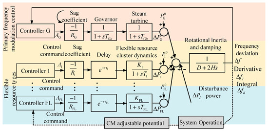
Figure 4. Different types of flexible resources participate in grid frequency coordination control.

The transfer function between the total response power of each frequency regulation unit and the flexible resource cluster and the system frequency can be expressed as follows:

$${\displaystyle \sum _{i_{\in \mathrm{G}}=1}^m\Delta }{P}_{\mathrm{G},i}(s)+{\displaystyle \sum _{j_{\in \mathrm{FL}}=1}^n\Delta }{P}_{\mathrm{FL},j}(s)-\Delta P_L(s)=\Delta f(s)(2Hs+D)$$

(32)

where $m$ and $n$ represent the numbers of the frequency regulation units and the flexible resource clusters, respectively; $\Delta P_{\mathrm{G},i}(s)$ and $\Delta P_{\mathrm{FL},j}(s)$ are the power variations of the i-th frequency regulation unit and the j-th flexible resource cluster; and $\Delta P_L(s)$ is the disturbance power, respectively.

3. Proposed Method

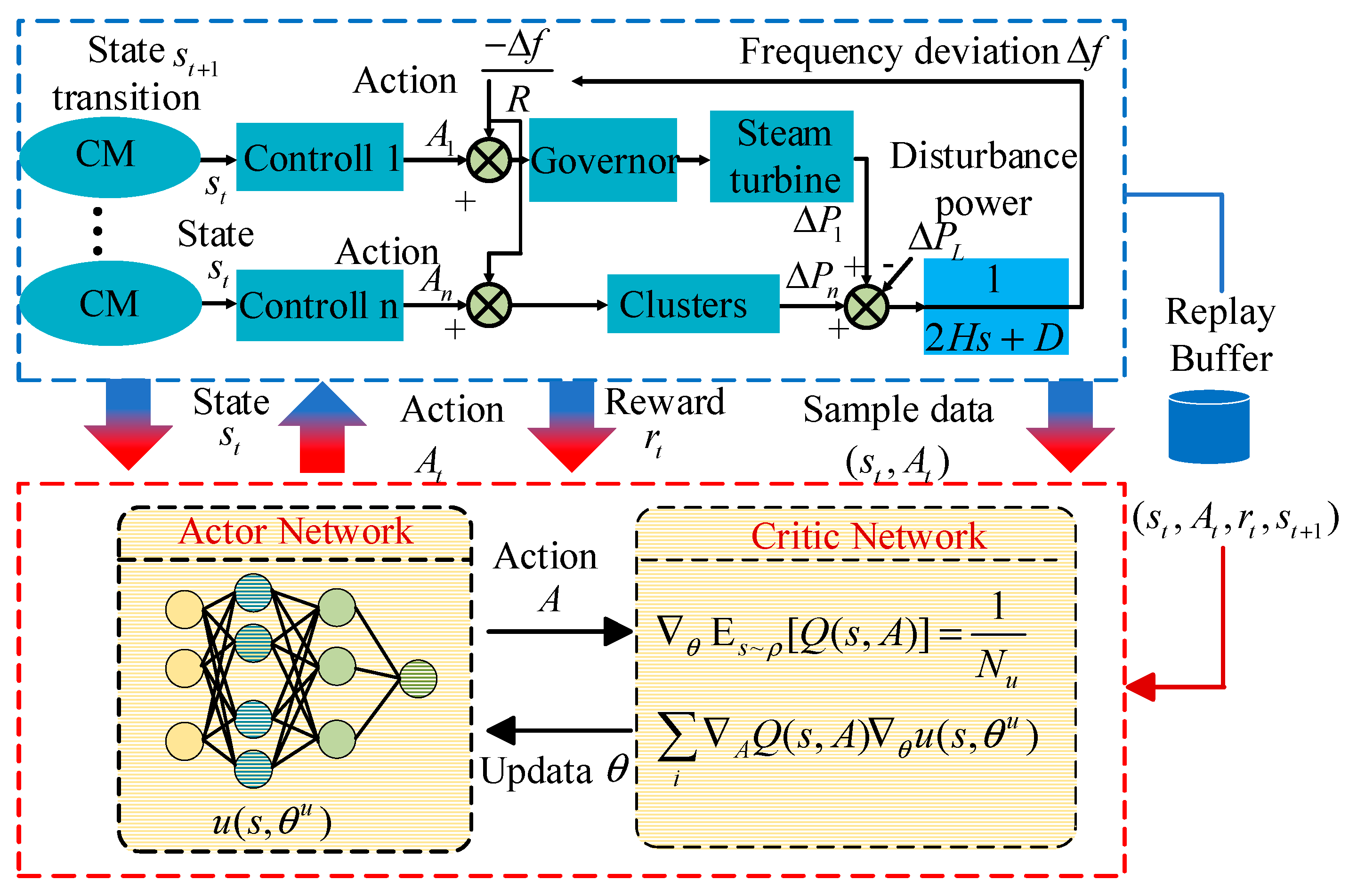
The DDPG algorithm adopted in this paper employs an “actor-critic” architecture. The proposed control model framework is shown in Figure 5. During the iterative computation at time step t, the actor first generates an action through the policy network $u(s,{\theta }^u)$ based on the observed state of the CM at this moment. Subsequently, the CM undergoes a state transition according to the control policy at this time, reaching the state $s_{t+1}$ at the next time step. Meanwhile, the reward $r_t$ at time t is fed back to the agent. The agent controller can obtain a large number of experience samples through interactions with the environment, which are stored in an experience replay buffer. These sample data are first input into the critic model, and ultimately used to update the agent’s network parameters $\theta$ in the form of policy gradients.

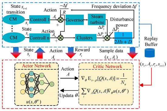
Figure 5. Frequency cooperative control principle model.

3.1. Control Objectives and Reward Functions

In this paper, the minimum of the sum of the weighted sum of the system frequency deviation and the total cost of the FM is taken as the control objective, and the optimal multi-intelligent body cooperative control strategy is formulated by taking the frequency stability and total cost of the FM into consideration.

A state-action value function $Q(s,A)$ is defined as follows to measure the system’s overall performance when every intelligence is working together to regulate it [32,33,34]:

$$\begin{array}{l}Q(s,A)=-\lambda [{\displaystyle \sum _{t=1}^T{\gamma }^t}{(\Delta f^{\ast }(t))}^2\Delta t]+\\ (1-\lambda )[{\displaystyle \sum _{t=1}^T(}{\displaystyle \sum _{i\in \mathrm{G}}^m\Delta }{P}_{\mathrm{G},i}^{\ast }(t)C_{\mathrm{G},i}^{\ast }\Delta t+{\displaystyle \sum _{j\in \mathrm{FL}}^n\Delta }{P}_{\mathrm{FL},j}^{\ast }(t)C_{\mathrm{FL},j}^{\ast }\Delta t)]\end{array}$$

(33)

$$r_i=-u_i|\Delta f_i|-w_1{C}_{\mathrm{FL},i}^{\ast }-w_2{(F_{\mathrm{SOC}}^{\mathrm{EV},i}-F_{\mathrm{SOCS}}^{\mathrm{EV}})}^2-w_3\Delta P_i^{\mathrm{base}}$$

(34)

where $Q(s,A)$ is the action value function; $\mathrm{G}$ and $\mathrm{FL}$ are the sets of the frequency regulation units and the flexible resource clusters, respectively; $m$ and $n$ represent the numbers of the frequency regulation units and the flexible resource clusters, respectively; $\Delta t$ and $T$ represent the size of the time step and the length of the experience trajectory, respectively; $s$ is the state information of the system; $\Delta P_{\mathrm{G},i}^{\ast }(t)$ and $\Delta P_{\mathrm{FL},j}^{\ast }(t)$ are the dimensionally unified outputs; $\Delta f^{\ast }(t)$ is the dimensionally unified frequency deviation; $C_{\mathrm{G},i}^{\ast }$ is the unit power output cost of the generator unit; $C_{\mathrm{FL},j}^{\ast }$ is the unit power output cost of the flexible resource cluster; and $\lambda$ is the weighting coefficient of the reward function. Since the reward function includes the frequency control effect and the frequency regulation cost, the applicability of the algorithm can be tested by comparing different proportions. Additionally, a discount factor $\gamma \in (0,1)$ is included in this study to ensure that the current frequency deviation is given more weight than future ones and that the system frequency deviation can be removed as quickly as possible. This study aims to lower the power system’s frequency regulation cost while maintaining the frequency control effect by prioritizing the power system’s frequency control effect over the economy. $r_i$ is the reward function of the agent; $|\Delta f_i|$ is the frequency deviation; $u_i$ and $w_1$ are the weights corresponding to the frequency regulation effect and the frequency regulation economy; $w_2$ is the penalty coefficient for the EV cluster deviating from the target; $w_3$ is the penalty coefficient for the change in the power reference value of the ACs cluster; $\Delta P_i^{\mathrm{base}}$ is the change in the power reference value of the i-th ACs cluster; $F_{\mathrm{SOC}}^{\mathrm{EV},i}$ is the state of charge of the i-th EVs; and $F_{\mathrm{SOCS}}^{\mathrm{EV}}$ is the set value of the state of charge of the EVs.

3.2. Actor Network Parameter Update Method

The optimal control action is obtained by maximizing the expected state-action value function $E_{s~\rho }[Q(s,A)]$ as the evaluation index. Thus, this study uses the chain derivation method to calculate the gradient of the expected state-action value function to the parameter $\theta =[{\theta }^{u_1},{\theta }^{u_2},\dots ,{\theta }^{u_{m+n}}]$ sequentially based on the gradient ascent algorithm concept. The iteratively updated parameter reaches its greatest value along the gradient of the expected state-action value function, resulting in the network parameter that allows each strategy network to output the best action. The gradient and its accompanying parameters are updated in the following manner.

$$\begin{array}{cc}\hfill {\nabla }_{{\theta }^{u_j}}{E}_{s~\rho }[Q(s,A)]& \approx {\displaystyle \frac{1}{N_u}}{\displaystyle \sum _i{\nabla }_{{\theta }^{u_j}}Q(s,A)}{|}_{s=s_i}\hfill \\ & ={\displaystyle \frac{1}{N_u}}{\displaystyle \sum _i{\nabla }_{A_j}Q(s,A)}{\nabla }_{{\theta }^{u_j}}{u}_j(s,{\theta }^{u_j}){|}_{s=s_i}\hfill \end{array}$$

(35)

$${\theta }^{u_j}\leftarrow {\theta }^{u_j}+\eta {\nabla }_{{\theta }^{u_j}}{E}_{s~\rho }[Q(s,A)]$$

(36)

where $\eta \in (0,1)$ is the learning rate of the policy network parameter ${\theta }^{u_j}$ and $N_u$ is the number of small batch sampling samples; the gradient of the expected state-action value function to parameter is approximated by averaging the gradient of the $N$ state-action value functions to the parameter.

To update parameters, ${\nabla }_{A_j}Q(s,A)$ and ${\nabla }_{\theta }{u}_j(s,{\theta }^{u_j})$ should be obtained first. The function expression of ${\nabla }_{\theta }{u}_j(s,{\theta }^{u_j})$ in the policy network is as follows:

$${\nabla }_{{\theta }^{u_j}}{u}_j(s;{\theta }^{u_j})={\nabla }_{{\theta }^{u_j}}(f_{{\theta }^{(n)}}^{(p)}[\cdot \cdot f_{{\theta }^{(1)}}^{(1)}(s)])$$

(37)

where $p$ represents the number of layers of the neural network; state $s$ is the input of the neural network; and $f_{{\theta }^{(l)}}^{(l)}$ denotes the activation function.

During the iterative updating of the network parameters, in order to find the gradient of the expectation of the state-action value function with respect to the parameters, it is crucial to obtain the gradient of the state-action value function with respect to the controller action.

According to the chain rule of differentiation, for the $i\in G$ FM unit, the following is obtained:

$$\begin{array}{cc}\hfill {\nabla }_{A_{i\in \mathrm{G}}}{Q}^{u_{i\in \mathrm{G}}}(s,A)=& -[2\lambda {\displaystyle \sum _{t=1}^T{\gamma }^t\Delta f(t)}{\nabla }_{A_{i\in \mathrm{G}}}{\displaystyle \frac{\Delta f(t)}{f_0^2}}\Delta t\hfill \\ & +(1-\lambda ){\displaystyle \sum _{t=1}^T{\nabla }_{A_{i\in \mathrm{G}}}\frac{\Delta P_{\mathrm{G},i}(t)C_i^{\mathrm{G}}}{P_0{C}_0}\Delta t}]\hfill \end{array}$$

(38)

For the $j\in \mathrm{FL}$ flexible resource cluster, the following is obtained:

$$\begin{array}{cc}\hfill {\nabla }_{A_{j\in \mathrm{FL}}}{Q}^{u_{j\in \mathrm{FL}}}(s,A)=& -[2\lambda {\displaystyle \sum _{t=1}^T{\gamma }^t\Delta f(t)}{\nabla }_{A_{j\in \mathrm{FL}}}{\displaystyle \frac{\Delta f(t)}{f_0^2}}\Delta t\hfill \\ & +(1-\lambda ){\displaystyle \sum _{t=1}^T{\nabla }_{A_{j\in \mathrm{FL}}}\frac{\Delta P_{\mathrm{FL},j}(t)C_j^{\mathrm{FL}}}{P_0{C}_0}\Delta t}]\hfill \end{array}$$

(39)

where $P_0$, $C_0$, and $f_0$ denote the datum values used for normalization when unifying the scale.

According to the knowledge of the frequency response model, the transfer function between the system frequency deviation, the FM unit, and the flexible resource controller output command can be expressed in the following form:

$$\begin{array}{cc}\hfill \Delta f(s)(2Hs+D)& ={\displaystyle {\sum }_{i=1,i\in \mathrm{G}}^m[}{A}_i(s)-{\displaystyle \frac{\Delta f(s)}{R_i}}]\hfill \\ & +{\displaystyle \frac{{\displaystyle {\sum }_{j=1,j\in \mathrm{FL}}^n{k}_{\mathrm{FL},j}}[A_j(s)-\frac{\Delta f(s)}{R_j}]}{(1+s{T}_{\mathrm{FL}})}}-\Delta P_L\hfill \end{array}$$

(40)

When compared to the generator set, the flexible resource cluster’s time constant is essentially insignificant.

The actual active output of FM units and flexible resource clusters is regulated by the sag control factor and controller output. Maximum and minimum output power limits must also be met. The maximum/minimum output power constraint of the generator and the flexible resource cluster can be further expressed as follows:

$$P_{\mathrm{G}/\mathrm{FL},j}^{\min }\le P_{\mathrm{G}/\mathrm{FL},j}^0+A_j-{\displaystyle \frac{\Delta f}{R_j}}\le P_{\mathrm{G}/\mathrm{FL},j}^{\max }$$

(41)

where $P_{\mathrm{G}/\mathrm{FL}}^0$, $P_{\mathrm{G}/\mathrm{FL}}^{\min }$, and $P_{\mathrm{G}/\mathrm{FL}}^{\max }$ denote the base operating point, the minimum output power constraint, and the maximum output power constraint.

Let $P_{\mathrm{G}/\mathrm{FL},j}=P_{\mathrm{G}/\mathrm{FL},j}^0+A_j-{\displaystyle \frac{\Delta f}{R_j}}$, while considering $A_j=u_j(s;{\theta }^{u_j})$; then, the following is an expression for the $P_{\mathrm{G}/\mathrm{FL},j}$ gradient about the network parameters:

$$\begin{array}{cc}\hfill {\nabla }_{{\theta }^{u_j}}{P}_{\mathrm{G}/\mathrm{FL},j}& ={\nabla }_{{\theta }^{u_j}}{A}_j-{\displaystyle \frac{1}{R_j}}{\nabla }_{{\theta }^{u_j}}\Delta f\hfill \\ & ={\nabla }_{{\theta }^{u_j}}{u}_j(s;{\theta }^{u_j})(1-{\displaystyle \frac{{\nabla }_{A_j}\Delta f}{R_j}})\hfill \end{array}$$

(42)

From Equation (31), the policy network parameter ${\theta }^{u_j}$ is updated along the following direction. Then, the corresponding generator and flexible resource cluster power output increases; conversely, the power output decreases.

$${\theta }^{u_j}\leftarrow {\theta }^{u_j}+\eta {\nabla }_{{\theta }^{u_j}}{P}_{\mathrm{G}/\mathrm{FL},j}$$

(43)

In combination with the ascending direction of the gradient given by Equation (36) and the generator power constraint, the final rules for updating the strategy network parameter are derived. The flexible resource cluster output is obtained as follows:

$${\theta }^{u_j}\leftarrow \left\{\begin{array}{l}{\theta }^{u_j}+\eta {\nabla }_{{\theta }^{u_j}}{E}_{s~\rho }[Q(s,A)],P_{\mathrm{G}/\mathrm{FL},j}^{\min }<P_{\mathrm{G}/\mathrm{FL},j}<P_{\mathrm{G}/\mathrm{FL},j}^{\max }\\ {\theta }^{u_j}+\eta \{{\nabla }_{{\theta }^{u_j}}{E}_{s~\rho }[Q(s,A)]-\\ {\displaystyle \frac{{\nabla }_{{\theta }^{u_j}}{E}_{s~\rho }[Q(s,A)]{\nabla }_{{\theta }^{u_j}}{P}_{\mathrm{G}/\mathrm{FL},j}}{{‖{\nabla }_{{\theta }^{u_j}}{P}_{\mathrm{G}/\mathrm{FL},j}‖}^2}}{\nabla }_{{\theta }^{u_j}}{P}_{\mathrm{G}/\mathrm{FL},j},else\end{array}\right.$$

(44)

The aforementioned equations demonstrate that the output power of the generating units and flexible resource clusters surpasses the limit if the parameter is updated in the gradient direction of the expected state-action value function to the parameter. To ensure that the trajectory of the parameter update is always within the feasible domain delineated by the frequency control model, the parameters will be updated in the subsequent iteration in the same direction as the projection of the expectation of the vector state-action value function on the plane normal to the vector ${\nabla }_{{\theta }^u}{P}_{\mathrm{G}/\mathrm{FL},j}$.

4. System Studies

4.1. Test System

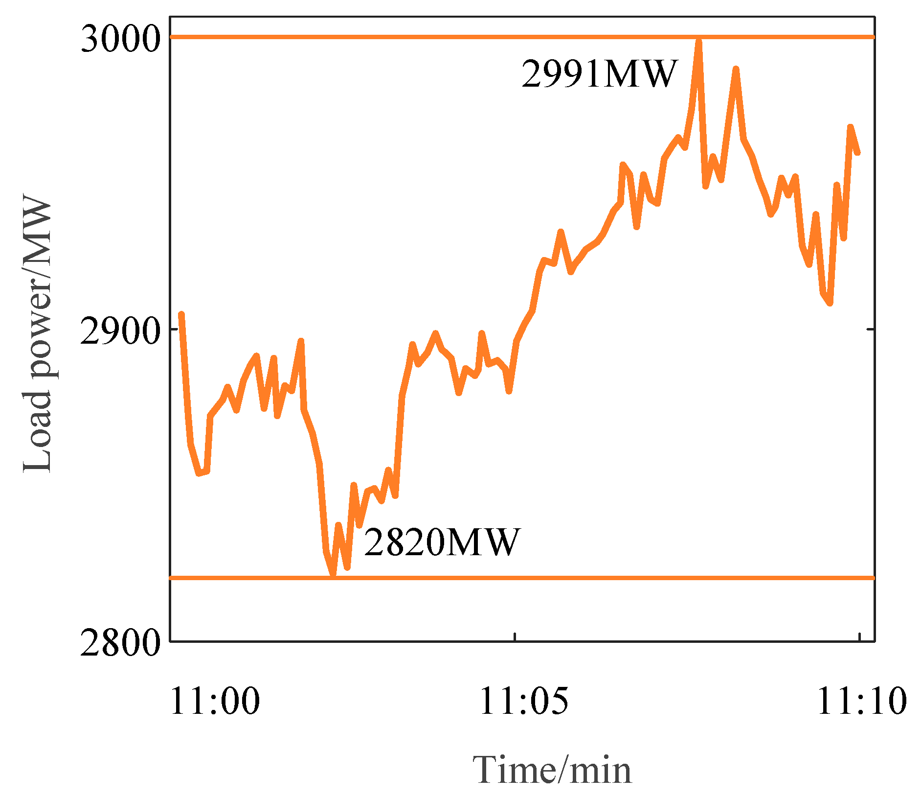
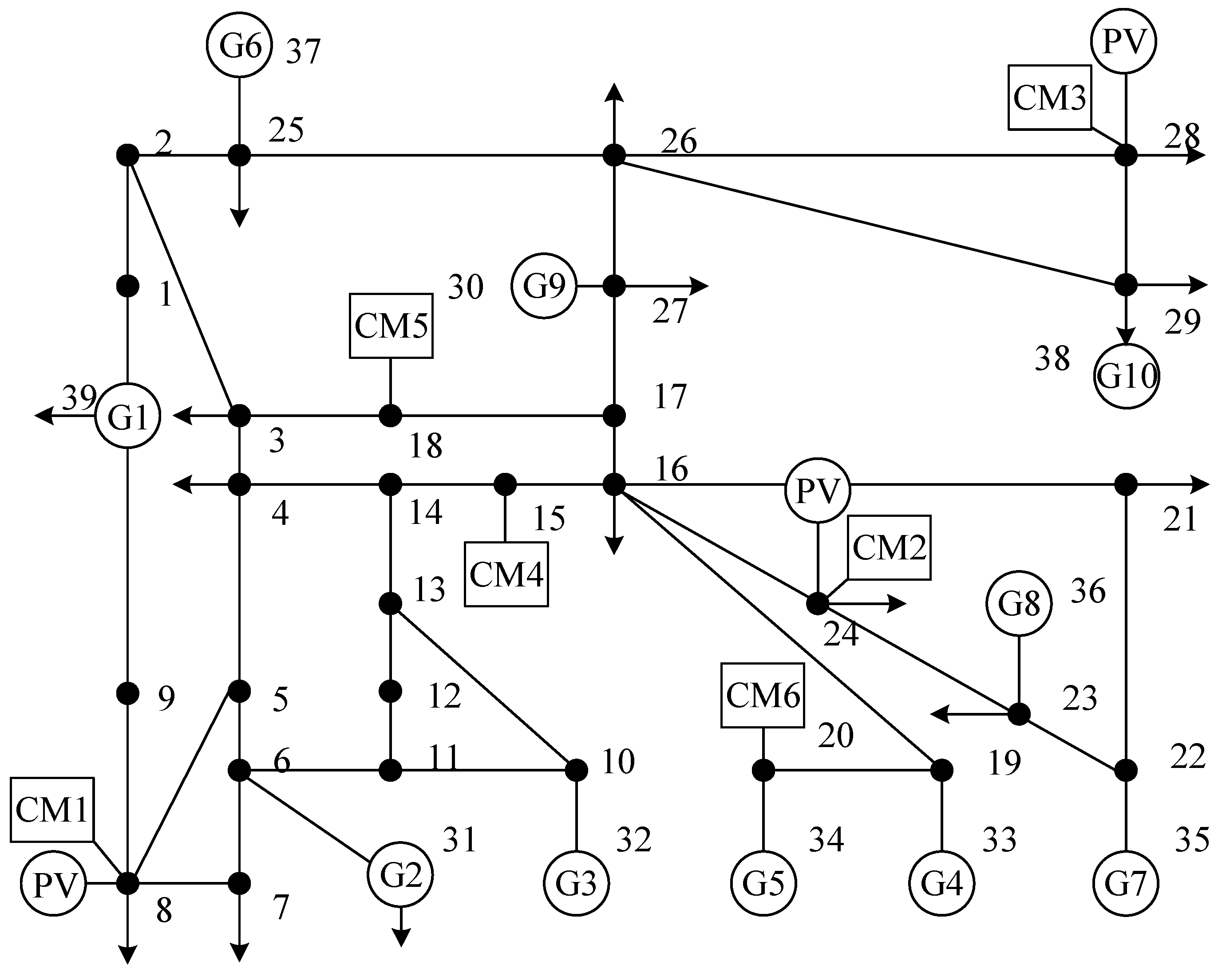
This case simulation focuses on a 39-node power system. This system not only has ten traditional generators that are all in grid-connected operation status, but also includes three EV clusters, three AC clusters, and three PV power plants, respectively, connected to nodes eight, twenty-four, and twenty-eight. Among them, the droop coefficients, governor inertia time constants, and other parameters of different traditional generators vary significantly, and their ramp characteristics and unit power generation costs also differ. The parameter settings refer to reference [35]. The system load is a dynamic active load. The power fluctuation curve within 10 min is shown in Figure 6, with the power fluctuation range being from 2820 MW to 2991 MW, which is used to simulate the change in the active power demand. The load damping coefficient is set to one. For the flexibility resources in the system, intelligent agent control units are established to achieve the coordinated control of large-scale flexible resources. The AC and EV clusters are modeled using the proposed CM in this paper, and a unified first-order inertia link describes their dynamic characteristics. During the simulation, all control commands need to undergo a power boundary check by the CM to ensure that the commands comply with physical and user constraints. In addition, the parameter values, output power reference values, maximum charge and discharge powers, and unit power scheduling costs of the flexible resources are listed in Table 1 and Table 2, respectively. The reference power, power upper and lower limits, unit power scheduling cost, regulation factor, and inertia time constant of the generator sets are listed in Table 3.

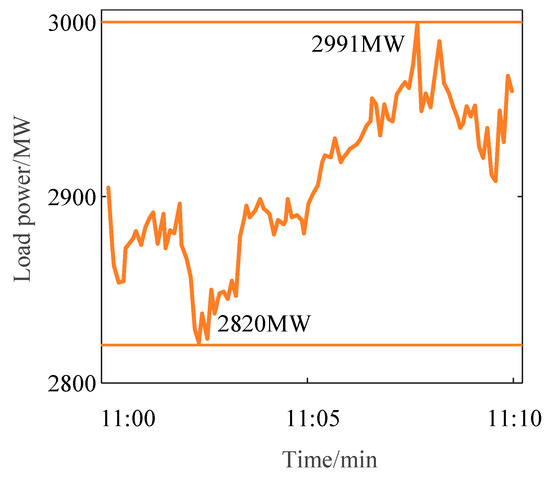
Figure 6. Load power within 10 min.

Table 1. Parameter detting of different resources.

Architectural-AC Parameters
Thermal capacity/(kJ/°C)	690.87	Initial set temperature /(°C)	25
Thermal resistance/(°C/kW)	7.12	Outdoor temperature /(°C)	33
EV Parameters
Energy consumption per kilometer ((kW·h) kW−1)	0.149	Charge state upper limit (%)	90
EV charging and discharging efficiency (%)	95	Lower limit of charging status (%)	10
Expected state of charge at home (%)	70	Expected state of charge when leaving home (%)	40

Table 2. Parameters for different flexible resources.

Parameter	Value
EV charge/discharge power (MW)	25, 28
EV discharge cost (yuan/MWh)	90
EV charge cost (yuan/MWh)	95
AC charge/discharge power (MW)	20, 24.5
AC discharge cost (yuan/MWh)	75
AC Charge cost (yuan/MWh)	79

Table 3. Parameter settings for generator sets.

Genset	Minimum Output Power/MW	Maximum Output Power/MW	Generation Costs/(yuan/MWh)	Base Power/MW	Regulation Factor/p.u.	Inertia Time Constant/s
G1	150	1000	35	500	3.5	5.5
G2	150	1000	35	500	3.5	5.5
G3	90	600	40	300	4	4.5
G4	90	600	40	300	4	4.5
G5	90	600	40	300	4	4.5
G6	50	350	60	200	4.5	3.5
G7	50	350	60	200	4.5	3.5
G8	30	180	75	100	5	2.5
G9	30	180	75	100	5	2.5
G10	30	180	75	100	5	2.5

As shown in Figure 7, six CMs are deployed in groups by resource type: CM1–CM3 are responsible for the charging/discharging coordination of EV clusters, which correspond to the PV-connected nodes due to the energy storage characteristics of EVs; CM4–CM6 are responsible for the power regulation of AC clusters, which correspond to the nodes with concentrated loads due to the load characteristics of ACs.

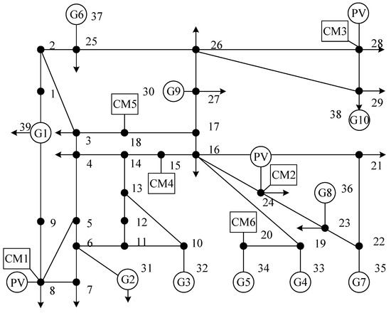
Figure 7. 39-node power system.

The simulation was implement in MATLAB/Simulink, running in the 2022b enviroment with a Core i7-10875H CPU, 32GB of memory and NVIDIA GeForce GTX 1650 Ti GPU.

To verify the effectiveness of the proposed algorithm for the real-time control of the system frequency in large-scale grid-connected scenarios of new energy, this section compares the control performance of several commonly used algorithms, which are based on the DQN algorithm for reinforcement learning and the DDPG algorithm. The reward decay rate, sampling period, and number of learning iterations of the DQN algorithm are set to 0.7, 0.1 s, and 800 episodes, respectively. It should be noted that the DQN algorithm employs a discrete action space, which means that when facing continuously varying system states, its action selection is coarse-grained and unable to achieve precise adjustment, thus resulting in limited control accuracy. The DDPG parameter settings are the same as in reference [36], with a training iteration of 800 times. It should be noted that the algorithm does not incorporate a constraint penalty term, which may generate actions violating practical constraints during the control process. Under the scenario of the large-scale integration of renewable energy, this could cause the operation of some devices in the system to exceed safety limits or optimal operating ranges, thereby affecting the system’s stability and reliability. The parameter settings for the proposed algorithm, including the number of experience trajectories M, the capacity of the experience replay pool D, the number of small batch sampling samples N, the learning rate $\eta$, discount factor $\lambda$, and intelligence g, are shown in Table 4.

Table 4. Parameter setting.

Parameter	M	D	N	$\mathit{\eta }$	$\mathit{\gamma }$	g
Values	500	6400	32	0.03	0.95	16

4.2. System Random and Load Perturbation

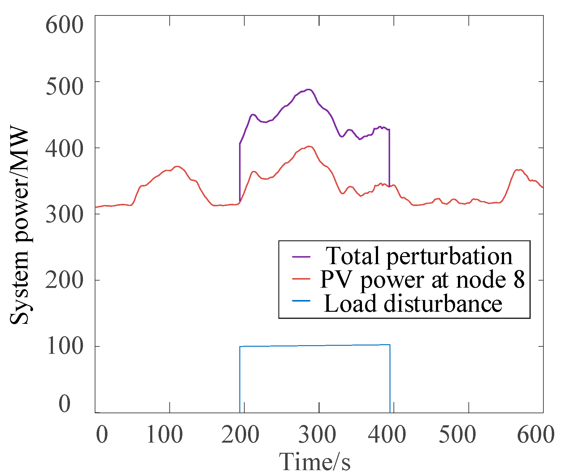
To simulate the operation of a complex interconnected power system, the section uses the load disturbance and PV output as simulations, and the simulation time is 600 s, as shown in Figure 8. The rectangular load disturbance, serving as an idealized step model in simulations, is used to verify the algorithm’s response capability to sudden disturbances and can be extended to more complex load fluctuation scenarios in practical applications [37,38,39].

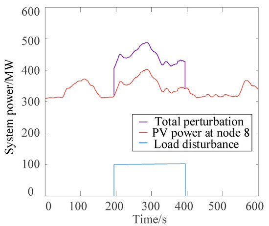
Figure 8. Strong random interference to the system.

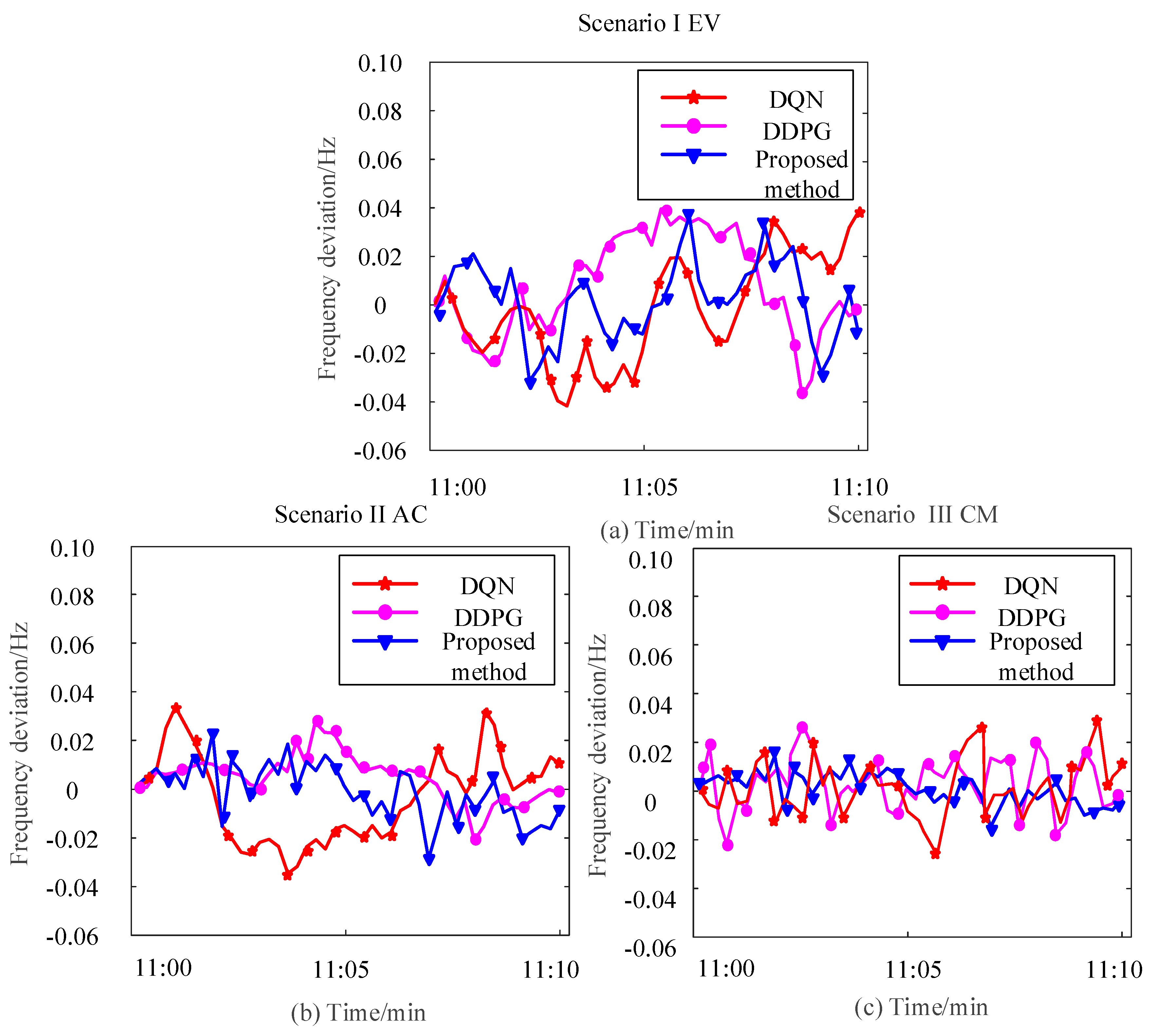
Figure 9 illustrates the dynamic response curves of system frequency deviations under different control algorithms across three scenarios. To ensure the clear presentation of curve trends and completely avoid marker symbols from obscuring data fluctuations, some markers were removed. The horizontal axis denotes time (600 s), while the vertical axis represents frequency deviation (Hz). Red, orange, and blue curves correspond to the control performance of DQN, DDPG, and the proposed method, respectively. The simulation scenarios include the following: the EVs only (Scenario I), the ACs only (Scenario II), and the clustered CM participation (Scenario III). The results demonstrate that while the DQN algorithm employs discrete action spaces, EV charging/discharging and AC power regulation inherently involve continuous variables. The DQN algorithm requires discretizing continuous control variables into finite actions, leading to insufficient power regulation precision and notable response hysteresis under dynamic disturbances. Although the DDPG algorithm operates in continuous action spaces, it fails to integrate the CM’s power/energy boundaries into its policy network or explicitly address multi-resource coordination, thereby struggling to optimize power allocation between EVs and ACs. To address these limitations, the proposed method employs a unified CM framework that comprehensively models the power constraints, energy constraints, and inertial characteristics of both EVs and ACs. By incorporating gradient projection optimization into policy network parameter updates, this approach ensures strict adherence to physical constraints while significantly reducing computational complexity. Under the three scenarios, the proposed strategy restricts frequency deviations to (−0.028 Hz, 0.030 Hz), (−0.021 Hz, 0.027 Hz), and (−0.017 Hz, 0.021 Hz), respectively. The comparative analysis demonstrates that the developed CM effectively suppresses frequency fluctuations in power systems. Both load clusters exhibit a substantial frequency regulation capacity throughout daily operations and participate in system frequency regulation with enhanced fault tolerance. This strategy provides a superior solution for frequency regulation challenges in renewable-dominated grids, particularly addressing the complexities of high renewable penetration. The proposed framework offers critical advantages in maintaining grid stability while optimizing multi-resource coordination.

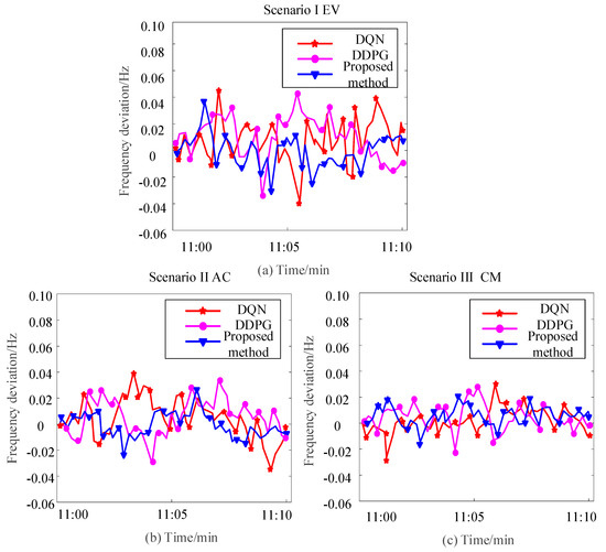
Figure 9. Frequency deviation of different scenarios under load and PV perturbations. The EVS only (Scenario I, (a)), the ACs only (Scenario II, (b)), and the clustered CM participation (Scenario III, (c)).

Table 5 reveals the core advantages of the CM in integrating two types of flexible resources—EVs and ACs: traditional methods (DQN/DDPG) exhibit limitations even in single scenarios. The DQN algorithm, constrained by its discrete action space, fundamentally stems from the mismatch between discrete regulation granularity and the continuous dynamic characteristics of devices. While the DDPG algorithm optimizes regulation accuracy through a continuous action space, it relies on indirect correction by reducing rewards after command violations occur. In contrast, the proposed method leverages the CM to minimize violations of system operation constraints via projected gradient descent, transforming independent resources into aggregate optimization within collaborative scenarios. This provides a feasible solution for the efficient participation of multi-type flexible resources in grid regulation.

Table 5. Comparison of algorithmic control effects in different scenarios.

Method	DQN	DDPG	Proposed Method
Scenario I	(−0.039, 0.046) Hz	(−0.034, 0.042) Hz	(−0.030, 0.035) Hz
Scenario II	(−0.035, 0.041) Hz	(−0.030, 0.035) Hz	(−0.024, 0.026) Hz
Scenario III	(−0.028, 0.030) Hz	(−0.021, 0.027) Hz	(−0.017, 0.021) Hz

To investigate the impact of different cluster scales on frequency control performance, this study establishes three AC clusters of varying scales: a small-scale cluster with 1000 individual ACs, a medium-scale cluster with 5000 units, and a large-scale cluster with 10,000 units.

As shown in Figure 10, the small-scale cluster exhibits significant individual differences, leading to the “overloading of some devices and idling of others” during regulation. This results in insufficient regulation power and only limited frequency support (frequency fluctuation range (−0.046, 0.048 Hz)), verifying the “small perturbation” characteristic of single loads. The medium-scale cluster transforms individual differences into “group-averaged characteristics” through collective effects, achieving a notable leap in regulation capability: compared with the small-scale cluster, its deviation suppression effect improves to (−0.035, 0.038 Hz), demonstrating the enhanced regulation capacity enabled by scaling. The large-scale cluster realizes a qualitative change in regulation capability, with its frequency fluctuation range narrowed to (−0.026, 0.025 Hz), proving that large-scale aggregation can transform AC clusters into critical regulatory resources for power systems. This phenomenon also validates the CM aggregation mechanism, i.e., the collective effect of load clusters narrows the frequency fluctuation range.

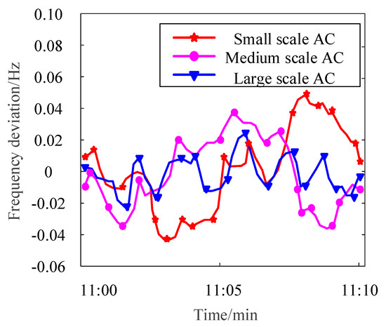
Figure 10. The frequency control effect of air conditioning units of different scales participating in frequency control.

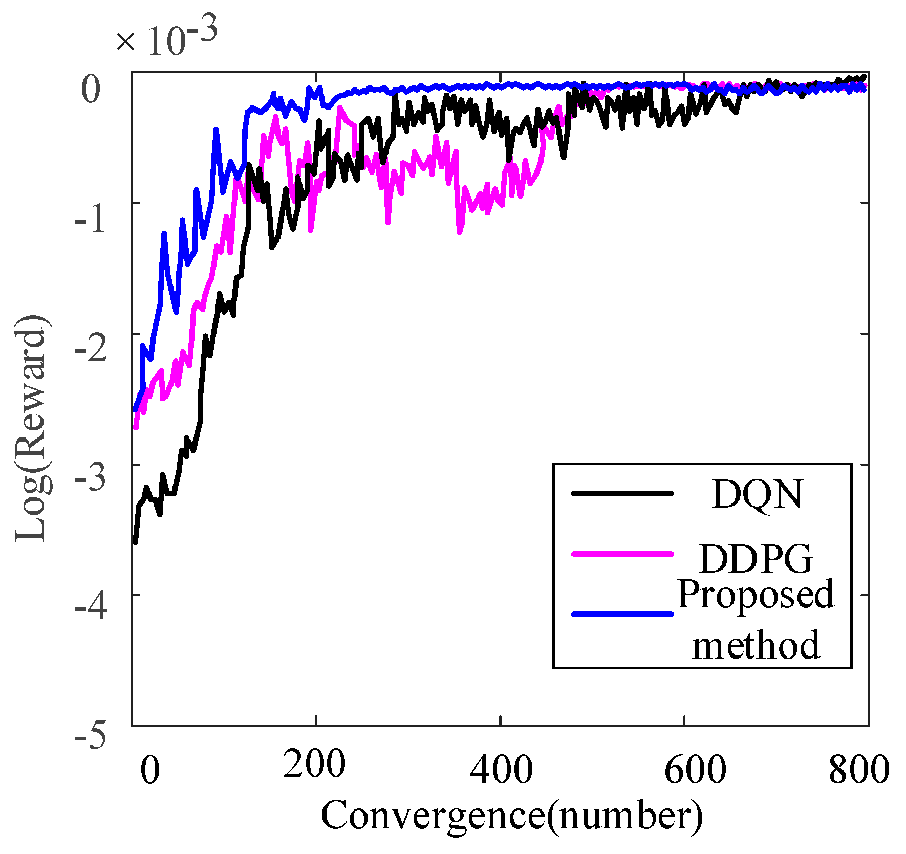
Figure 11 compares the cumulative reward value iterative convergence process of the DQN and DDPG algorithms, and the proposed method. The cumulative reward values of the DQN and DDPG algorithms tend to stabilize after 640 and 520 iterations. Notably, each iteration cycle contains an experience trajectory of 150 iterations, which means that the DQN and DDPG algorithms require 96,000 and 78,000 iterations, respectively, to converge. In contrast, the proposed method requires only 150 iterations (22,500 iterations updates) to complete the parameter training of deep neural networks. In addition, the convergence curve of the proposed algorithm has the smallest oscillation amplitude. The DDPG algorithm exhibits significantly lower cumulative rewards compared to the proposed method, accompanied by notable oscillations. This deficiency stems from its reliance on experience replay through random sampling, which disrupts the temporal correlations among power system states. Consequently, it demonstrates delayed learning in extreme operational scenarios and fails to incorporate the physical constraints of DSFRs, thereby frequently triggering penalty mechanisms. Meanwhile, the DQN approach suffers from insufficient control precision or dimensional catastrophes due to action space discretization, while its Q-value maximization strategy tends to overestimate action values, leading to policy deviation. In contrast, the proposed method calculates policy gradients in real-time via gradient optimization without relying on experience replay, and the projected gradient method ensures the feasibility of control commands, thereby avoiding penalty losses and enhancing the number of effective regulation instances. This verifies the superiority of the proposed strategy in complex power system control.

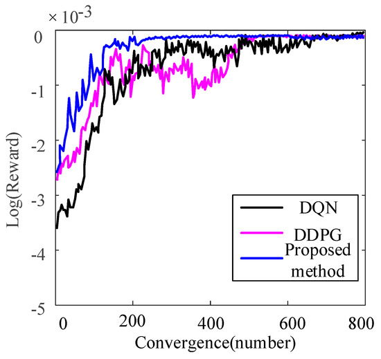
Figure 11. Convergence curves of different algorithms.

Table 6 gives a comparison of different algorithms in terms of system frequency deviation, training time, and decision time. The proposed algorithm improves over the DQN (43.8%, 66.2%, 20%) and DDPG (27.8%, 76.0%, 56.1%) algorithms in terms of frequency control, training time, and decision time. The proposed method has better frequency control under the interference of new energy and load, which can greatly reduce the time required for intensive learning training [37,38,39]. These advantages are attributed to the CM’s unified modeling of heterogeneous resources, reducing model complexity compared to traditional detailed state-space methods.

Table 6. Performance comparison of different algorithms under PV and load perturbations.

Performance Indicators	DQN	DDPG	Proposed Method
$\left|\overline{\Delta f}\right|$/Hz	0.025	0.021	0.015
t1/min	14.9	21.6	5.1
t2/s	0.0056	0.0088	0.0043

4.3. High Percentage of New Energy Disturbances

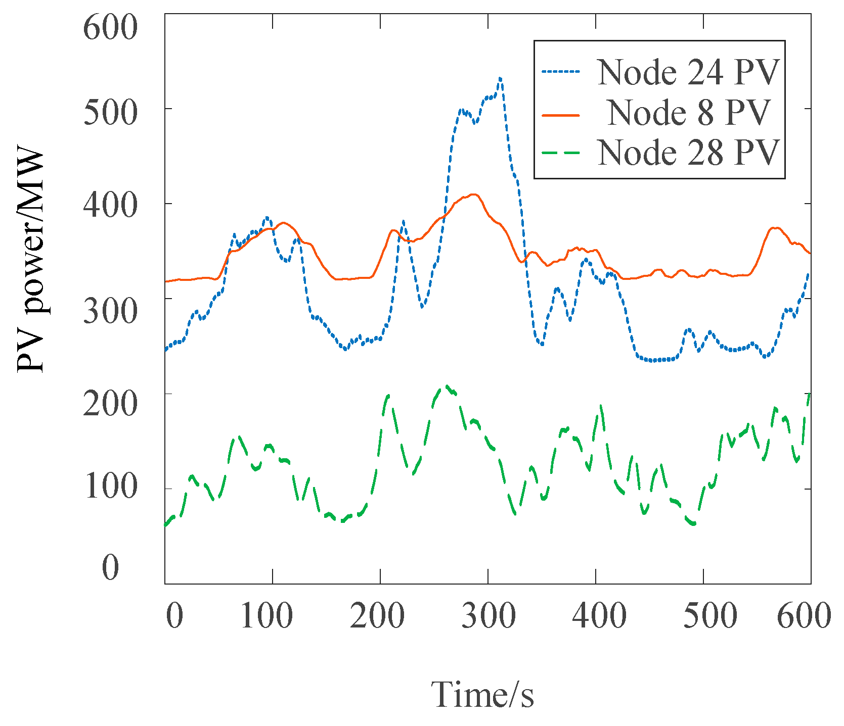
A high proportion of new energy has strong randomness. Only PV is considered as a random fluctuation in the system without considering the frequency regulation effect of the load to simulate the stochastic variations of a high percentage of new energy sources. The system with a steady-state initial state is subject to PV fluctuations at nodes eight, twenty-four, and twenty-eight, and the power fluctuations of the PV power station used are shown in the Figure 12.

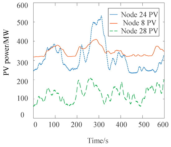
Figure 12. Dynamic power changes.

Figure 13 presents the system frequency variations of different algorithms under the scenario of high-proportion renewable energy random fluctuations, where only PV is used as the random fluctuation input, and the load frequency regulation effect is not considered. As shown in Figure 12, the PV fluctuations at nodes eight, twenty-four, and twenty-eight are the primary causes of frequency changes. It can be intuitively observed from the curves in Figure 13 that the frequency fluctuation curve of the proposed method is the smoothest. In contrast, the frequency fluctuation amplitudes of the DQN and DDPG algorithms are significantly larger. The proposed method can effectively suppress frequency fluctuations due to its unified modeling and optimization strategy, which enables it to quickly react to random PV fluctuations, adjust system power allocation, and stabilize the frequency. However, restricted by its discrete action space, the DQN algorithm cannot achieve fine-grained control during power regulation. Facing continuous random variations in PV, it struggles to quickly match appropriate actions, leading to larger frequency fluctuations. Since the DDPG algorithm does not effectively handle physical constraints, it fails to accurately coordinate the power output of each device when PV fluctuations change the system’s power demand, resulting in significant frequency fluctuations. These results demonstrate that the proposed method exhibits obvious advantages in frequency control under high-proportion renewable energy random fluctuation scenarios, providing a reliable solution for frequency stability control in high-proportion renewable energy power grids.

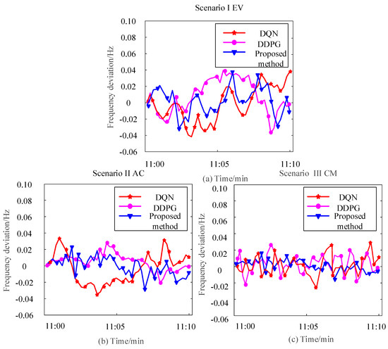
Figure 13. Frequency deviation in different scenarios under high-scale PV perturbation. The EVS only (Scenario I, (a)), the ACs only (Scenario II, (b)), and the clustered CM participation (Scenario III, (c)).

Data from Table 7 demonstrate that the proposed method exhibits significant advantages over the DQN algorithm (81.1%, 36.7%) and DDPG algorithm (50.0%, 29.6%) in terms of absolute frequency deviation and maximum frequency deviation, respectively. This is of great significance for actual system operation: taking absolute frequency deviation as an example, this advantage means that the average degree of system frequency deviation from the rated frequency is significantly reduced, minimizing impacts on the normal operation of various devices in the system. In scenarios with high-proportion renewable energy and random fluctuations, rapid changes in PV power pose a severe test to the algorithm’s control capabilities. Due to its discrete action space, the DQN algorithm struggles to achieve fast and precise power regulation in the face of frequent PV power fluctuations. For instance, when PV power fluctuates drastically over a short period, the DQN algorithm cannot select appropriate actions from its limited discrete action set for adjustment in a timely fashion, leading to large frequency deviations. Although the DDPG algorithm has a continuous action space, it lacks the effective handling of physical constraints. When PV fluctuations cause changes in system power demand, the DDPG algorithm fails to accurately coordinate power output. For example, during a sudden drop in PV power, the DDPG algorithm may not restrict the power consumption of certain devices, causing the system frequency to decline rapidly and resulting in significant frequency deviations. In contrast, the proposed method, leveraging unified modeling and optimized strategies, precisely adapts to random PV fluctuations, and rapidly responds to and suppresses frequency deviations. It fully considers the physical constraints of each device in the system, reasonably allocates power during PV fluctuations, maintains stable system operation, and ensures that frequency deviations remain at low levels.

Table 7. Performance comparison of different algorithms under high percentage of PV perturbations.

Performance Indicators	DQN	DDPG	Proposed Method
$\left|\overline{\Delta f}\right|$/Hz [37,38,39,40]	0.105	0.034	0.020
Max $\left|\Delta f\right|$	0.028	0.025	0.015
t1/min	15.2	24.4	6.3
t2/s	0.0113	0.0154	0.0096

The proposed method introduces the weighting factor $\lambda$ in the objective function to balance the frequency deviation control effect and the total system FM cost. The frequency and economic indicators under different weighting factors are shown in Table 8.

Table 8. Performance with different weighting factors.

Weighting Factor $\lambda$	1	0.8	0.6	0.4	0.2
$\left|\overline{\Delta f}\right|$ (Hz)	0.012	0.014	0.016	0.019	0.021
$\overline{F_G}$ (yuan)	5998	5904	5745	5803	5769

Table 8 presents the influence of the weight factors in the reward function on frequency deviation and regulation cost, reflecting the critical role of the CM in multi-objective optimization. When $\lambda$ = 1, the reward function prioritizes minimizing frequency deviation, and the CM’s power boundary constraints ensure that devices do not overload during extreme regulation, resulting in minimal frequency deviation but the highest total cost due to frequent activation of high-cost discharge resources. As $\lambda$ decreases, the system reduces reliance on high-cost resources, achieving a dynamic balance between frequency stability and economic regulation. This advantage stems from the CM’s unified modeling of heterogeneous resources and the reduction in trial-and-error costs during training.

5. Conclusions

This study proposed a multi-agent reinforcement learning framework integrating a CM to achieve the collaborative frequency control of multi-type DSFRs, such as EVs and ACs. By developing a unified modeling mechanism, the research translates the dynamic characteristics of heterogeneous resources and user constraints into computable collaborative regulation parameters. Considering the uncertainty of flexible resources, a frequency collaborative control model was constructed. The projected gradient descent algorithm was introduced to ensure that control commands meet real-time device physical boundaries and user demands. A state-aware multi-objective optimization strategy was further designed to dynamically adjust weight and penalty factors based on resource real-time states, achieving priority configuration for different objectives such as frequency stability, user constraints, and regulation economy. The proposed method enables the collaborative characterization of multi-resource dynamic behaviors, a reliable guarantee of control command feasibility, and the effective balance of multi-objective optimization. Simulation results demonstrate that this framework significantly enhances frequency regulation performance in complex scenarios, providing a novel solution for large-scale flexible resources to participate in grid regulation. It holds important value for promoting renewable energy integration and enhancing the flexibility regulation capability of power systems.

However, on the demand side, a large number of thermal, cooling, and gas energy resources also exhibit fast-response and equivalent energy storage characteristics. Future research should focus on analyzing how to incorporate more diverse resources into the model, integrating demand-side flexibility to provide multiple services for the power system. Additionally, this paper only uses the weighted sum of frequency regulation cost and performance in the reward function without a specific cost analysis. In practical scenarios, the relationship between frequency regulation cost and performance is more complex and requires further investigation.

References

- Fang, J.; Li, H.; Tang, Y.; Blaabjerg, F. On the Inertia of Future More-Electronics Power Systems. IEEE J. Emerg. Sel. Top. Power Electron. 2019, 7, 2130–2146. [Google Scholar] [CrossRef]
- Hu, P.; Li, Y.; Yu, Y.; Blaabjerg, F. Inertia estimation of renewable-energy-dominated power system. Renew. Sustain. Energy Rev. 2023, 183, 113481. [Google Scholar] [CrossRef]
- Moore, P.; Alimi, O.A.; Abu-Siada, A. A Review of System Strength and Inertia in Renewable-Energy-Dominated Grids: Challenges, Sustainability, and Solutions. Challenges 2025, 16, 12. [Google Scholar] [CrossRef]
- Yu, G.; Liu, C.; Tang, B.; Chen, R.; Lu, L.; Cui, C.; Hu, Y.; Shen, L.; Muyeen, S.M. Short term wind power prediction for regional wind farms based on spatial-temporal characteristic distribution. Renew. Energy 2022, 199, 599–612. [Google Scholar] [CrossRef]
- Yu, G.Z.; Lu, L.; Tang, B.; Wang, S.Y.; Chen, R.S.; Chung, C.Y. Ultra-short-term Wind Power Subsection Forecasting Method Based on Extreme Weather. IEEE Trans. Power Syst. 2022, 38, 5045–5056. [Google Scholar] [CrossRef]
- Azizi, S.; Sun, M.; Liu, G.; Terzija, V. Local Frequency-Based Estimation of the Rate of Change of Frequency of the Center of Inertia. IEEE Trans. Power Syst. 2020, 35, 4948–4951. [Google Scholar] [CrossRef]
- Liu, X.; Liu, Y.; Liu, J.; Xiang, Y.; Yuan, X. Optimal planning of AC-DC hybrid transmission and distributed energy resource system: Review and prospects. CSEE J. Power Energy Syst. 2019, 5, 409–422. [Google Scholar] [CrossRef]
- Shrivastava, S.; Khalid, S.; Nishad, D.K. Impact of EV interfacing on peak-shelving and frequency regulation in a microgrid. Sci. Rep. 2024, 14, 31514. [Google Scholar] [CrossRef]
- Zhao, H.; Wu, Q.; Huang, S.; Zhang, H.; Liu, Y.; Xue, Y. Hierarchical control of thermostatically controlled loads for primary frequency support. IEEE Trans. Smart Grid 2018, 9, 2986–2998. [Google Scholar] [CrossRef]
- Jendoubi, I.; Sheshyekani, K.; Dagdougui, H. Aggregation and optimal management of TCLs for frequency and voltage control of a microgrid. IEEE Trans. Power Deliv. 2021, 36, 2085–2096. [Google Scholar] [CrossRef]
- Yu, Z.; Bao, Y.; Yang, X. Day-ahead scheduling of air-conditioners based on equivalent energy storage model under temperature-set-point control. Appl. Energy 2024, 368, 123481. [Google Scholar] [CrossRef]
- Cai, L.; Yang, C.; Li, J.; Liu, Y.; Yan, J.; Zou, X. Study on Frequency-Response Optimization of Electric Vehicle Participation in Energy Storage Considering the Strong Uncertainty Model. World Electr. Veh. J. 2025, 16, 35. [Google Scholar] [CrossRef]
- Shukla; Rajan, R.; Garg, M.M.; Panda, A.K. Driving grid stability: Integrating electric vehicles and energy storage devices for efficient load frequency control in isolated hybrid microgrids. J. Energy Storage 2024, 89, 111654. [Google Scholar] [CrossRef]
- Wen, Y.; Hu, Z.; You, S.; Duan, X. Aggregate Feasible Region of DERs: Exact Formulation and Approximate Models. IEEE Trans. Smart Grid 2022, 13, 4405–4423. [Google Scholar] [CrossRef]
- Wang, S.; Wu, W. Aggregate Flexibility of Virtual Power Plants with Temporal Coupling Constraints. IEEE Trans. Smart Grid 2021, 12, 5043–5051. [Google Scholar] [CrossRef]
- Feng, C.; Chen, Q.; Wang, Y.; Kong, P.Y.; Gao, H.; Chen, S. Provision of Contingency Frequency Services for Virtual Power Plants with Aggregated Models. IEEE Trans. Smart Grid 2023, 14, 2798–2811. [Google Scholar] [CrossRef]
- Huang, X.; Li, K.; Xie, Y.; Liu, B.; Liu, J.; Liu, Z.; Mou, L. A novel multistage constant compressor speed control strategy of electric vehicle air conditioning system based on genetic algorithm. Energy 2022, 241, 122903. [Google Scholar] [CrossRef]
- Liu, W.; Tan, J.; Cui, J. Design of a PID Control Scheme for Pound-Drever–Hall Frequency-Tracking System Based on System Identification and Fuzzy Control. IEEE Sens. J. 2024, 24, 39252–39259. [Google Scholar] [CrossRef]
- He, L.; Tan, Z.; Li, Y.; Cao, Y.; Chen, C. A Coordinated Consensus Control Strategy for Distributed Battery Energy Storages Considering Different Frequency Control Demands. IEEE Trans. Sustain. Energy 2024, 15, 304–315. [Google Scholar] [CrossRef]
- Xie, J.; Sun, W. Distributional Deep Reinforcement Learning-Based Emergency Frequency Control. IEEE Trans. Power Syst. 2022, 37, 2720–2730. [Google Scholar] [CrossRef]
- Li, J.; Yu, T.; Cui, H. A multi-agent deep reinforcement learning-based “Octopus” cooperative load frequency control for an interconnected grid with various renewable units. Sustain. Energy Technol. Assess. 2022, 51, 101899. [Google Scholar] [CrossRef]
- Chen, X.; Zhang, M.; Wu, Z.; Wu, L.; Guan, X. Model-Free Load Frequency Control of Nonlinear Power Systems Based on Deep Reinforcement Learning. IEEE Trans. Ind. Inform. 2024, 20, 6825–6833. [Google Scholar] [CrossRef]
- Yu, L.; Sun, Y.; Xu, Z.; Shen, C.; Yue, D.; Jiang, T.; Guan, X. Multi-agent deep reinforcement learning for HVAC control in commercial buildings. IEEE Trans. Smart Grid 2021, 12, 407–419. [Google Scholar] [CrossRef]
- Sahu, P.C.; Baliarsingh, R.; Prusty, R.C.; Panda, S. Novel DQN optimised tilt fuzzy cascade controller for frequency stability of a tidal energy-based AC microgrid. Int. J. Ambient. Energy 2020, 43, 3587–3599. [Google Scholar] [CrossRef]
- Li, J.; Zhou, T. Prior Knowledge Incorporated Large-Scale Multiagent Deep Reinforcement Learning for Load Frequency Control of Isolated Microgrid Considering Multi-Structure Coordination. IEEE Trans. Ind. Inform. 2024, 20, 3923–3934. [Google Scholar] [CrossRef]
- Lee, W.-G.; Kim, H.-M. Deep Reinforcement Learning-Based Dynamic Droop Control Strategy for Real-Time Optimal Operation and Frequency Regulation. IEEE Trans. Sustain. Energy 2025, 16, 284–294. [Google Scholar] [CrossRef]
- Dobbe, R.; Hidalgo-Gonzalez, P.; Karagiannopoulos, S.; Henriquez-Auba, R.; Hug, G.; Callaway, D.S.; Tomlin, C.J. Learning to control in power systems: Design and analysis guidelines for concrete safety problems. Electr. Power Syst. Res. 2020, 189, 106615. [Google Scholar] [CrossRef]
- Zhang, Z.; Zhang, D.; Qiu, R.C. Deep reinforcement learning for power system applications: An overview. CSEE J. Power Energy Syst. 2019, 6, 213–225. [Google Scholar]
- Hao, H.; Somani, A.; Lian, J.; Carroll, T.E. Generalized aggregation and coordination of residential loads in a smart community. In Proceedings of the 2015 IEEE International Conference on Smart Grid Communications (SmartGridComm), Miami, FL, USA, 2–5 November 2015; pp. 67–72. [Google Scholar] [CrossRef]
- Hao, H.; Wu, D.; Lian, J.; Yang, T. Optimal Coordination of Building Loads and Energy Storage for Power Grid and End User Services. IEEE Trans. Smart Grid 2018, 9, 4335–4345. [Google Scholar] [CrossRef]
- Ulbig, A.; Andersson, G. Analyzing operational flexibility of electric power systems. In Proceedings of the 2014 Power Systems Computation Conference, Wroclaw, Poland, 18–22 August 2014; pp. 1–8. [Google Scholar] [CrossRef]
- Yu, P.; Zhang, H.; Song, Y.; Hui, H.; Huang, C. Frequency Regulation Capacity Offering of District Cooling System: An Intrinsic-Motivated Reinforcement Learning Method. IEEE Trans. Smart Grid 2023, 14, 2762–2773. [Google Scholar] [CrossRef]
- Yu, P.; Zhang, H.; Song, Y. Adaptive Tie-Line Power Smoothing with Renewable Generation Based on Risk-Aware Reinforcement Learning. IEEE Trans. Power Syst. 2024, 39, 6819–6832. [Google Scholar] [CrossRef]
- Yu, P.; Zhang, H.; Song, Y.; Hui, H.; Chen, G. District Cooling System Control for Providing Operating Reserve Based on Safe Deep Reinforcement Learning. IEEE Trans. Power Syst. 2024, 39, 40–52. [Google Scholar] [CrossRef]
- Moeini, A. Open data IEEE test systems implemented in SimPower Systems for education and research in power grid dynamics and control. In Proceedings of the 2015 50th International Universities Power Engineering Conference, Stoke on Trent, UK, 3 December 2015; pp. 1–6. [Google Scholar]
- Lowe, R.; Wu, Y.; Tamar, A.; Harb, J.; Abbeel, P.; Mordatch, I. Multi-Agent Actor-Critic for Mixed Cooperative-Competitive Environments. arXiv 2020, arXiv:170602275. [Google Scholar]
- Yang, F.; Huang, D.; Li, D.; Lin, S.; Muyeen, S.M.; Zhai, H. Data-Driven Load Frequency Control Based on Multi-Agent Reinforcement Learning with Attention Mechanism. IEEE Trans. Power Syst. 2023, 38, 5560–5569. [Google Scholar] [CrossRef]
- Zhang, G.; Li, J.; Xing, Y.; Bamisile, O.; Huang, Q. Data-driven load frequency cooperative control for multi-area power system integrated with VSCs and EV aggregators under cyber-attacks. ISA Trans. 2023, 143, 440–457. [Google Scholar] [CrossRef]
- Yan, Z.; Xu, Y. A Multi-Agent Deep Reinforcement Learning Method for Cooperative Load Frequency Control of a Multi-Area Power System. IEEE Trans. Power Syst. 2020, 35, 4599–4608. [Google Scholar] [CrossRef]
- Wu, Z.; Lv, Z.; Huang, X.; Li, Z. Data driven frequency control of isolated microgrids based on priority experience replay soft deep reinforcement learning algorithm. Energy Rep. 2024, 11, 2484–2492. [Google Scholar] [CrossRef]
Disclaimer/Publisher’s Note: The statements, opinions and data contained in all publications are solely those of the individual author(s) and contributor(s) and not of MDPI and/or the editor(s). MDPI and/or the editor(s) disclaim responsibility for any injury to people or property resulting from any ideas, methods, instructions or products referred to in the content. |
© 2025 by the authors. Licensee MDPI, Basel, Switzerland. This article is an open access article distributed under the terms and conditions of the Creative Commons Attribution (CC BY) license (https://creativecommons.org/licenses/by/4.0/).