Discrimination of High Impedance Fault in Microgrids: A Rule-Based Ensemble Approach with Supervised Data Discretisation

Abstract

This research presents a voting ensemble classification model to distinguish high impedance faults (HIFs) from other transients in a photovoltaic (PV) integrated microgrid (MG). Due to their low fault current magnitudes, sporadic incidence, and non-linear character, HIFs are difficult to detect with a conventional protective system. A machine learning (ML)-based ensemble classifier is used in this work to classify HIF more accurately. The ensemble classifier improves overall accuracy by combining the strengths of many rule-based models; this decreases the likelihood of overfitting and increases the robustness of classification. The ensemble classifier includes a classification process into two steps. The first phase extracts features from HIFs and other transient signals using the discrete wavelet transform (DWT) technique. A supervised discretisation approach is then used to discretise these attributes. Using discretised features, the rule-based classifiers like decision tree (DT), Java repeated incremental pruning (JRIP), and partial decision tree (PART) are trained in the second phase. In the classification step, the voting ensemble technique applies the rule of an average probability over the output predictions of rule-based classifiers to obtain the final target of classes. Under standard test conditions (STCs) and real-time weather circumstances, the ensemble technique surpasses individual classifiers in accuracy (95%), HIF detection success rate (93.3%), and overall performance metrics. Feature discretisation boosts classification accuracy to 98.75% and HIF detection to 95%. Additionally, the ensemble model’s efficacy is confirmed by classifying HIF from other transients in the IEEE 13-bus standard network. Furthermore, the ensemble model performs well, even with noisy event data. The proposed model provides higher classification accuracy in both PV-connected MG and IEEE 13 bus networks, allowing power systems to have effective protection against faults with improved reliability.

1. Introduction

Microgrids (MGs) provide reliable, affordable, and robust electricity to local and rural places [1]. However, integrating various distributed generation (DG) sources, such as conventional, nonlinear, and intermittent renewable energy (RE) sources, and anomalous events caused by switching heavy loads and various faults like high impedance fault (HIF) and low impedance (LI) faults in the MG network can negatively impact security and reliability [2]. The HIF has a low fault current amplitude, making it difficult to detect and isolate using typical protective relays. MG networks often experience HIF when the conductor touches high-resistance materials like wet sand, asphalt, tree limbs, gravels, etc. [3]. The HIF current’s intermittent, asymmetric, non-linear, and arcing properties increase the risk of electrical shock and fire, damage the healthy MG network, and induce cascading failure [4,5]. In this instance, a protective system that accurately detects and discriminates HIF in the MG network is needed to isolate the problematic piece faster and more precisely [6]. Hence, to expedite and enhance the precision of identifying the problematic network segment, it is imperative to employ an advanced protection system that relies on the reliable detection and discrimination of HIFs. In this regard, advanced machine learning (ML) classifiers offer interesting possibilities for detecting and distinguishing HIF in power systems with better accuracy and reliability [6]. As a result, ML approaches are prominent among researchers for detecting and distinguishing HIFs in power systems.

During the initial processing stage of ML-based classification, scholars have employed various signal processing methods (SPMs) to extract the dataset’s features from event signals [7,8,9,10,11]. In numerous works, the wavelet transform (WT) method is extensively utilised for feature extraction due to its simplicity and adaptability in analysing the non-stationary characteristics of fault transient signals in both time and frequency domains simultaneously [12]. In comparison to conventional methods, the discrete WT (DWT) approach, a variant of WT, has the advantages of being more accurate and requiring less time to process signals during feature extraction [13,14]. Feature discretisation is another important process in the preprocessing phase of classification. The discretisation technique transforms the attribute values from a continuous dataset into a discrete collection of intervals. The discretisation technique is also helpful in the selection of features that can improve classifier performance when working with high-dimensional data [15,16]. Discretisation is simple, quick to implement, and improves learning precision and speed. There are two types of discretisation: supervised discretisation and unsupervised discretisation. On datasets with information on class labels, information entropy, or mean class values, supervised discretisation is used. Unsupervised discretisation is performed on datasets with no class information, and discrete data can be generated using two methods: equal width binning and equal frequency binning. The unsupervised technique may not yield adequate results when the distribution of continuous data is not uniform. Furthermore, it is susceptible to outliers, which have a significant impact on the ranges. In this instance, the supervised discretisation method can be used to compensate for the unsupervised method’s drawbacks [17]. Among the different discretisation algorithms in the literature, Fayyad and Irani’s [18] entropy-based discretisation method is popular and has produced excellent results. As a result, in this study, during the preprocessing phase, the DWT methodology is used for feature extraction, the supervised discretisation filter (based on the Fayyad–Irani method) is accessible with Waikato Environment for Knowledge Analysis (WEKA), and an open source tool is used for discretisation.

The researchers employed a variety of ML algorithms to detect and categorise HIFs in the MG and radial power distribution networks. For the classification of HIFs in radial power distribution networks, classifiers such as Decision Tree (DT) [19], Artificial Neural Network (ANN) [20,21], Support Vector Machine (SVM) [22,23], Multi-Layer Perceptron (MLP) [24], Convolutional Neural Network (CNN) [6], Back Propagation Neural Network (BPNN) [25], and Probabilistic Neural Network (PNN) [26] have been used. Moreover, Naïve Bayes (NB) [27] has been utilised to classify HIFs from other transients in MG networks, and the utilisation of mathematical morphology techniques and LSTM Recurrent neural networks have been considered in PV-integrated power networks [14,28]. According to the majority of research studies [29], a single weak classifier can only provide successful results for a particular type of application, and every classifier described in the literature has its own advantages and disadvantages. Ensemble classifiers may be employed in such circumstances to augment the predictive capabilities of a single weak classifier. By training multiple classifiers to tackle a common problem, ensemble models enhance the precision and consistency of single weak classifiers [29]. The boosting method [30], bagged tree [31] and random forest (RF) [32] are the examples of ensemble classifiers utilised by the researchers to categorise multiple electrical failures in different power systems. To further differentiate HIF in PV-integrated power networks, ensemble classifiers based on the extended Kalman filter with RF [33] and the K-nearest neighbours (KNNs)-based random subspace (RS) technique [3] have been used. According to the study, ensemble classifiers are more reliable and provide better classification performance than individual weak classifiers. The simple, highly efficient, and widely applied bagging and boosting ensemble algorithms use a set of homogenous weak classifiers in classification tasks. As an alternative, a voting strategy of an ensemble classifier is built using a group of heterogeneous weak classifiers. This method outperforms ensemble models like bagging and boosting to achieve the maximum generalisation accuracy in classification [13,34]. As a result, this work recommends using a voting approach of ensemble classifier to detect and categorise HIFs from other transient events.

For this proposed voting approach of ensemble classifier, rule-based classifiers (DT, JRIP, and PART) have been used in the first phase of classification, because of their distinct benefits in interpretability, computing efficiency, and appropriateness for the special issues of HIF detection. These rule-based classifiers provide clear, human-readable decision rules, essential for comprehending and verifying fault patterns in power systems, hence providing transparency and confidence in the task of fault classification. Moreover, rule-based classifiers are computationally efficient, making them suitable for real-time applications that need minimal latency and optimal resource utilisation. Advanced ensemble classifiers such as Random Forest (RF) and Gradient Boosting (GB) function as “black-box” models and need substantial processing resources. Random Forests (RF) and Gradient Boosting (GB) are effective for general-purpose classification tasks that include intricate, nonlinear connections; nevertheless, their deficiencies in interpretability, elevated computing requirements, and restricted adaptability to unbalanced and domain-specific datasets make them less appropriate for HIF classification [35]. Also, there is a dearth of research on the classification of HIFs in the RE-integrated MG power system using heterogeneous ensemble classifiers with the adoption of feature discretisation. Furthermore, no research has been discovered that evaluates HIFs using a voting approach of the ensemble technique in the context of real-time uncertainty caused by the integration of RE sources in the MG power system. The suggested voting ensemble method is used to distinguish HIFs from other transient occurrences for the islanded MG network under standard test conditions (STCs) and the real-time solar intermittency of the PV system. The following are the study’s main contributions:

• To identify and differentiate HIFs from other transients in a solar PV-integrated MG and IEEE 13 bus network models, a heterogeneous-based voting ensemble model is recommended.
• Applying the discrete wavelet transform (DWT) technique, the features are retrieved from HIF and other transient signals of the MG network.
• Using the supervised discretisation method, the extracted features from the DWT analysis are discretised before learning the ensemble and rule-based individual classifiers.
• The proposed ensemble model’s effectiveness is evaluated by comparing classification accuracy, the successive rate of HIFs, and performance indices (PI) for the ensemble and rule-based individual classifiers under STC and weather intermittency of solar PV in an islanded MG network.
• The proposed ensemble model’s classification accuracy and success rate of HIF are analysed under the noisy environment of even signals.
• A classification study for HIFs and other transients in the IEEE 13 bus standard network is also considered to validate the effectiveness of the suggested ensemble model.

The manuscript is structured as follows: The examined MG model and IEEE 13 bus network model are described in detail in Section 2, the configuration of the HIF model is explained in Section 3, and the processes involved in the classification procedure are laid out in Section 4. The initial processing of event signals and dataset are discussed in Section 5. The methodology is described in Section 6, with specifics on the proposed voting ensemble classifiers and rule-based individual classifiers. Results from the classification and sensitivity analyses are discussed in Section 7, and a conclusion and directions for further work are provided in Section 8.

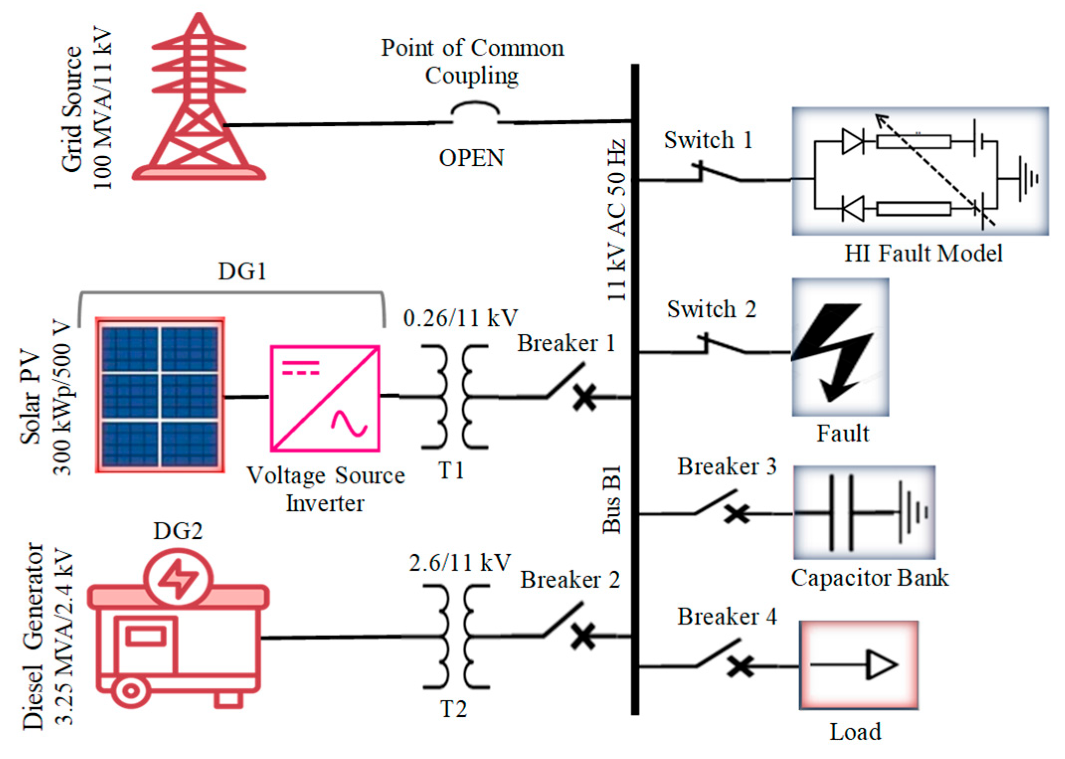
2. Models Studied: PV Connected MG and IEEE 13 Bus Network

The MG model, as shown in Figure 1, is created using the Matlab-Simulink software (2019b version) tool with the following configuration:

• Mode of MG operation: Islanded (point of common coupling breaker open in Grid side);
• Distributed generation source (DG1): Solar PV 300 kWp rated capacity with the implementation of two converters (DC–DC boost converter (280 V/500 V) and DC–AC Inverter (500 V DC/260V AC)) and interconnecting Transformer T1 (0.260 kV/11 kV);
• Distributed generation source (DG2): Diesel engine generator (3.25 MVA, 2.6 kV) with interconnecting transformer T2 (2.6 kV/11 kV);
• Interconnected AC load capacity: maximum 2400 kW (11 kV);
• Maximum capacity of interconnected capacitor bank: maximum 600 kVAR (11 kV);
• Low impedance (LI) faults introduction (line to ground (LG), line to line ground (LLG), all three lines to ground (LLLG), and line to line (LL)) with varying values of fault resistance;
• High-impedance fault (HIF) model configuration: Configured with anti-parallel diodes (D1 and D2), variable resistors (R1 and R2), and variable voltage sources (V1 and V2).

The IEEE 13 bus network model, as shown in Figure 2, consists of 13 buses and these buses are interconnected with different feeders. The line parameters are followed and the connection between load and generation sources is made as per the configuration details presented in [36]. The network model is modified with interconnection: of following elements:

• The network model (operating voltage 4.16 kV) is connected to the source of main grid (100 MVA, 4.16 kV, 50 Hz);
• A 300 kWp capacity of solar PV unit is connected at bus node 680 of network model;
• The interconnecting transformer (300 kVA, 0.26 kV/4.16 kV) integrates the solar PV unit (which includes a boost converter (DC–DC) and voltage source inverter (DC–AC)) at bus node number 680 of the IEEE 13-bus network.

3. Configuration of Studied High Impedance (HI) Fault Model

The comparable circuit and nonlinearity of the voltage–current curves of the HIF model are shown in Figure 3a,b. A collection of anti-parallel diodes, tuneable resistors, and DC source voltages are components of the HIF model [33]. The Emanuel model is emulated by the HIF model circuit [24]. In the HIF model, nonlinear voltage–current curves can be generated by adjusting R1 and R2 resistance values and V1 and V2 voltage levels, as described in Section 2. The network model’s HIF voltage and current patterns are nonlinear, asymmetrical, low-amplitude, and dominated by second- and third-order harmonics.

The current signal samples of various events are collected using the same procedure in both the MG model and the IEEE 13 bus network. The following procedure (

Table 1. Procedure for generating samples of current signals with various events.

High Impedance Fault
Range of Resistance Values (R1 and R2)	Range of Voltage Level (V1 and V2)	Characteristics of HIF Current	Method of Variation	Type of Surface
0.12 kΩ to 1.2 kΩ	0.5 kV to 3.2 kV	High current and sustained arc	Resistance values varied randomly	Wet soil
0.8 kΩ to 2.2 kΩ	3.5 kV to 6.5 kV	Moderate current build-up and arc	Voltage +/−5% Resistance +/−10%	Grass
1.5 kΩ to 3 kΩ	4.2 kV to 7.5 kV	Low, intermittent arc sustain	step change +/−10% in R1/R2 per half cycle	Asphalt wet
2.3 kΩ to 4 kΩ	5.2 kV to 8.5 kV	Low current and arc extinction frequent	R1/R2 values randomly varied every 2 ms	Dry soil
3 kΩ to 5.2 kΩ	6.2 kV to 10 kV	sporadic arc and very low current (less than 5 amps)	R1/R2 values randomly varied every 10 ms	Dry concrete
Low Impedance (LI) Fault
Varying fault resistances between 8 Ω and 115 Ω in various time steps
Capacitor switching transient (CST)
Switching on capacitor between 200 kVAR and 600 kVAR in different time steps
Load switching transient (LST)
Switching on load between 500 kW and 2400 kW in different time steps

) generates approximately 960 current signal samples (120 samples per event) for analysis during the simulation of network models (total simulation time 0.5 s).

4. Overview of the Classification Process

An overview of the classification process is shown in Figure 4. The PV connected MG and IEEE 13 bus network models are simulated in the simulation stage while HIF and other transients are present. During the data collection stage, current signals from various occurrences are measured and stored. The features are retrieved from the stored signals of various events through the DWT approach. Using the supervised method of discretisation, first the discretised features are used to learn the rule-based classifiers DT, JRIP, and PART. Then, the predictions from the rule-based classifiers are computed and applied with the average probability of voting to get the targeted class labels in the final stage.

5. Initial Processing of Event Signals and Dataset

In preprocessing stage, first the features of the dataset are generated by decomposing the current signals of various faults and transient events using discrete wavelet transform (DWT) technique. Then, the numeric data of retrieved features are transformed into nominal data by assigning numeric values into distinct groups through discretisation. The concept of DWT and discretisation techniques are described in this section, as follows.

5.1. Decomposing Signals Using Discrete Wavelet Transform (DWT) Method

Breaking signals into time and frequency domain parts is better with the wavelet transform (WT) than with other signal processing methods [13]. The WT method has two variants: continuous WT (CWT) and discrete WT (DWT). DWT easily solves constraints like insufficient redundancy and CWT’s inapplicability to real-time applications. DWT is defined as follows: [37]

$$\mathrm{D}\mathrm{W}\mathrm{T}(\mathrm{q},\mathrm{k})={\displaystyle \frac{1}{\sqrt{{\mathrm{b}}_{\mathrm{o}}^{\mathrm{q}}}}}{\displaystyle \sum _{\mathrm{s}}\mathrm{x}(\mathrm{s})\times \mathrm{g}}\times \left({\displaystyle \frac{\mathrm{k}-\mathrm{s}\mathrm{a}{\mathrm{b}}_{\mathrm{o}}^{\mathrm{q}}}{{\mathrm{b}}_{\mathrm{o}}^{\mathrm{q}}}}\right)$$

(1)

where ${\mathrm{b}}_{\mathrm{o}}^{\mathrm{q}}$ represents the scaling parameter, $\mathrm{s}{\mathrm{b}}_{\mathrm{o}}^{\mathrm{q}}$ stands for the translation parameter, g stands for the function of the mother wavelet, q and s stand for integer variables, x(s) stands for the time signal, and k stands for the sample number in an input signal. The input test signal x (s) for the DWT method can be divided into approximation and detailed coefficients using multi-resolution analysis (MRA). Equations (2) to (4), respectively, yield the co-efficient and evaluation of energy value (EV) expressions [34]. In this work, the mother wavelet’s Daubechies 4 (db4) function and the fifth decomposition level are taken into account as the main elements for the decomposition of signals. The previously published work explains additional DWT approach information [13].

$${\mathrm{A}}_{\mathrm{i}}(\mathrm{s})={\displaystyle \sum _{\mathrm{k}}\mathrm{x}(\mathrm{s})\times \mathrm{L}\mathrm{F}\mathrm{T}1}\times \left(2\mathrm{s}-\mathrm{k}\right)$$

(2)

$${\mathrm{D}}_{\mathrm{J}}(\mathrm{s})={\displaystyle \sum _{\mathrm{k}}\mathrm{x}(\mathrm{s})\times \mathrm{H}\mathrm{F}\mathrm{T}1}\times \left(2\mathrm{s}-\mathrm{k}\right)$$

(3)

$$\mathrm{E}\mathrm{V}={\displaystyle \sum _{\mathrm{J}=1}^{\mathrm{N}}[|{\mathrm{D}}_{\mathrm{J}}{|}^2]}+|{\mathrm{A}}_{\mathrm{N}}{|}^2$$

(4)

where ${\mathrm{A}}_{\mathrm{i}}$ and ${\mathrm{D}}_{\mathrm{J}}$ stand for the approximation and detailed coefficients, respectively, N represents the decomposition level, and LFT1 and HFT1 denote low-pass and high-pass filters, respectively.

5.2. Feature Discretisation

The attribute values of continuous data can be discretised into a finite set of intervals using data discretisation. Additionally, discretisation serves as a technique for choosing variables (features), significantly affecting the efficiency of classification algorithms used in the investigation of complex, high-dimensional datasets [15,16]. Discretisation is simple, easy to apply, and makes the learning more precise and faster. There are two types of discretisation, namely supervised and unsupervised discretisation. Supervised discretisation is applied on datasets with information of class labels, information entropy, or mean class values. While unsupervised discretisation is used on datasets with no class information, discrete data can be created in two ways: equal width binning and equal frequency binning. When the distribution of the continuous data is not uniform, the unsupervised technique might not produce satisfactory results. Furthermore, it is subject to outliers, which have a major impact on the ranges [17]. In this case, a supervised discretisation method can be utilised to compensate for the limitations of the unsupervised method.

The discretisation procedure typically consists of three phases: sorting the continuous values of the variable to be discretised, evaluating various cut points based on a given criterion, and terminating the search when a stop condition is fulfilled. Among the various discretisation algorithms in the literature, entropy-based techniques have typically shown outstanding results. Entropy-based discretisation is one of the commonly used supervised discretisation methods introduced by Fayyad and Irani [18]. In this study, the supervised discretisation filter (based on the Fayyad–Irani method) available with WEKA is utilised for the discretisation of data in the preprocessing phase. The class entropy of candidate partitions determines the discretisation cut point in the proposed supervised discretisation. The process of discretisation is described as follows [38,39]:

• First, the continuous values of features (X_N) are converted into k discrete intervals {[dI0, dI1], [dI1, dI2], …, (dIK-1, dIK]}, in that dI0 and dIK are the minimum and maximum values of the feature X.
• Then, to discretise feature X_N, the data are sorted by increasing the value of the feature.
• In the given dataset of DS, with the consideration of feature X_N and cut point T_P, the class entropy which is partitioned with T_P (random select) can be expressed as

$$\mathrm{E}({\mathrm{X}}_{\mathrm{N}},{\mathrm{T}}_{\mathrm{P}},\mathrm{D}\mathrm{S})={\displaystyle \frac{\left|\mathrm{D}{\mathrm{S}}_1\right|}{\mathrm{D}\mathrm{S}}}\mathrm{E}\mathrm{n}\mathrm{t}(\mathrm{D}{\mathrm{S}}_1)+{\displaystyle \frac{\left|\mathrm{D}{\mathrm{S}}_2\right|}{\mathrm{D}\mathrm{S}}}\mathrm{E}\mathrm{n}\mathrm{t}(\mathrm{D}{\mathrm{S}}_2)$$

(5)

where $\mathrm{D}{\mathrm{S}}_1$ and $\mathrm{D}{\mathrm{S}}_2$ are two subsets of the dataset DS partitioned by T_P, and Ent(DS) is the entropy of the output class that can be evaluated as follows:

$$\mathrm{E}\mathrm{n}\mathrm{t}(\mathrm{D}\mathrm{S})=-{\displaystyle \sum _{\mathrm{J}=1}^{\mathrm{N}}\mathrm{P}}({\mathrm{C}}_{\mathrm{J}},\mathrm{D}\mathrm{S})\log (\mathrm{p}({\mathrm{C}}_{\mathrm{J}},\mathrm{D}\mathrm{S}))$$

(6)

where ${\mathrm{C}}_{\mathrm{J}}$, … ${\mathrm{C}}_{\mathrm{N}}$ are N output classes and P(CJ, DS) is the probability distribution of class ${\mathrm{C}}_{\mathrm{J}}$ in dataset DS. A value of T_P that minimises the entropy of Equation (5) is selected as a cut point from among all the candidate cut points. This process is repeated until a termination criterion is met. In this work, the retrieved features of energy values (EA, EB, and EC) from the current signals of all three phases are used as an input dataset. A sample of discretised features (EA) generated by WEKA’s discretisation filter is illustrated in

Table 2. Discretisation of features.

Range	Number of Subset	Class
{-inf–50,350,000}	12	Capacitor switching transient (CST)
{50,350,000–50,800,000}	5	High iImpedance fault (HIF)
{50,800,000–55,250,000}	10	Load switching transient (LST)
{55,250,000–2,924,850,000}	3	High impedance fault (HIF)
{2,924,850,000–5,805,000,000}	10	Normal
{5,805,000,000–5,885,000,000}	4	Line to line ground (LLG)
{5,885,000,000–5,955,000,000}	11	Line to ground (LG)
{5,955,000,000–6,000,000,000}	9	Line to line (LL)
{6,000,000,000–6,600,000,000}	6	All the lines to ground (LLLG)
{6,600,000,000–inf}	10	All the lines to ground (LLLG)

.

6. Classification Methodology

The research uses the WEKA (version 3.9.6) program to categorise HIF from other transient events in an islanded MG network. The tool offers supervised and unsupervised machine learning methods, including the grouping, visualisation, regression, and classification [23]. Various events in the MG network are considered and classified with the PS1 to PS8 class names. The study also discusses individual rule-based and proposed ensemble classifiers.

6.1. Decision Table (DT)

The DT classifier is a simple algorithm suitable for smaller datasets with discrete attributes. It uses a table format to describe complex logic more precisely. The algorithm consists of a collection of features and a set of labelled classes. It creates rules based on the relationships between attribute values and class labels. When a specific instance contains multiple matching rules, the DT classifier uses a unique resolution strategy to determine the final class label. To obtain appropriate attribute combinations, the best-first search approach is used in this work [40,41]. A fundamental concept of the DT classification process is expressed as follows:

$$\mathrm{L}\mathrm{S}=\mathrm{f}(\mathrm{A}\mathrm{X})=\mathrm{R}(\mathrm{A}\mathrm{X})$$

(7)

where LS denotes targeted class labels, f stands for decision function, AX states for input feature values (AX = (AX₁, AX₂, …, AX_N)), and R specifies a set of decision rules where each rule describes the condition for the combination of feature values and class labels.

6.2. Java Repeated Incremental Pruning (JRIP)

The JRIP algorithm uses the Repeated Incremental Pruning to Produce Error Reduction (Ripper) method, an improved version of the Incremental Reduced Error Pruning (IREP) algorithm. Ripper is a rule-based learning method that constructs rules to discriminate class labels while minimising error. It is more efficient than the decision tree classifier for large and noisy datasets. The algorithm involves four stages: growth, pruning, optimisation, and selection, with growth involving greedily adding conditions for better performance [16]. During this process, the greatest information gain (IG), which is expressed in the Equation (8), can be achieved by selecting the appropriate condition for each attribute value [16].

$$\mathrm{I}\mathrm{G}=\mathrm{p}1\times \left(\log {\displaystyle \frac{\mathrm{p}1}{\mathrm{t}\mathrm{r}}}-\log {\displaystyle \frac{\mathrm{p}1}{\mathrm{T}\mathrm{c}}}\right)$$

(8)

where p1 denotes the number of positive examples covered by the rule, tr stands for the total number of positive and negative examples covered by the rule, and Tc states the total number of positive and negative examples in each class. The Weka algorithm uses a pruning phase to identify a rule that maximises the rule value metric by removing conditions in reverse order. The optimisation phase refines the rules by adding new attributes or rules. The selection phase retains the best rules, discarding the rest. In Weka, three folds are set, one for pruning and the rest for growing rules, and five optimisation runs are considered [16].

6.3. Partial Decision Tree (PART)

The PART technique is a method that combines the divide-and-conquer strategy for learning decision trees with the separate-and-conquer strategy for learning rules [16]. It generates decision lists, ordered sets of rules, and recursively creates rules for remaining instances [42]. The PART approach is computationally efficient as it does not attempt to find the globally optimal attribute at each node, but instead chooses the attribute with the best accuracy on the current data subset [43]. The PART algorithm, from WEKA, allows users to control the generated tree by setting parameters like the minimum number of instances needed to split a node, the confidence threshold, and the number of folds permitted during pruning [44]. In this work, the PART classifier is used with confidence factor 0.25, the number of folds with dataset 3, and the number of instances per leaf 2.

6.4. Proposed Ensemble Classifier

The proposed ensemble classification model, as shown in Figure 5, consists of two stages: training rule-based classifiers like DT, JRIP, and PART using a preprocessed dataset and a 10-fold cross-validation strategy, and acquiring the final targeted class labels from PS1 to PS8, which are then classified using a meta-level classification method using a voting rule of the “average of probabilities” to generate initial level output predictions. The average probabilities technique (soft voting) in a voting ensemble combines predictions by averaging class probabilities from each base classifier. The ensemble determines each class’s average probability and chooses the class with the highest average as the final forecast, resulting in more accurate and reliable outcomes compared to majority voting.

The steps involved in the proposed ensemble classifier’s classification process are given as follows:

Step (a): Formulate the input training dataset (TD_S) as per the strategy of the cross-validation approach.

• Training dataset TD_S is partitioned into 10 equally sized subsets using the 10-fold cross-validation method: TD_S = (TD_S1, TD_S2, TDS3, …, TDSK); (k = 10).

Step (b): Rule-based classifiers (RC1, RC2, …, RCN) are trained on allocated subsets at the first level of classification.

• Three rule-based classifiers, such as DT (RC1), JRIP (RC2), and PART (RC3) (N = 3), are trained in the initial stage of classification.

Step (c): The rule-based classifier output predictions (PRC1, PRC2, and PRC3) are computed with the voting rule in the second stage.

Step (d): According to the predictions from the rule-based classifier (RC), the probability distribution vector (PRC) for the specified dataset (dx) with various class names ((PS1, PS3, PS3, …, PSM); (M = 8)) can be expressed as follows [34]:

$$\mathrm{PRC}(\mathrm{dx})=\mathrm{PRC}(\mathrm{PS}1|\mathrm{X}),\mathrm{PRC}(\mathrm{PS}2|\mathrm{X}),\dots ,\mathrm{PRC}(\mathrm{PSM}|\mathrm{X})$$

(9)

Step (e): The probability distribution vectors of rule-based classifiers are merged or averaged through the application of the voting technique to obtain the class probability distribution of the suggested ensemble classifier.

• The rule of voting technique “average of probabilities” is applied and described as [45]:

$$\mathrm{P}\mathrm{R}{\mathrm{C}}_{\mathrm{M}\mathrm{C}}(\mathrm{x})={\displaystyle \sum _{\mathrm{C}=1}^{\mathrm{N}}\frac{1}{\mathrm{N}}\mathrm{P}\mathrm{R}\mathrm{C}(\mathrm{X})}$$

(10)

for a given set of input samples (X), the rule-based classifier’s (RC) probability distribution is denoted by PRC(X), the set of classifiers is defined by C = (1, 2, …, N), probability estimation averaging function is denoted by ${\displaystyle \frac{1}{N}}$, and the class probability distribution of the proposed voting classifier is stated by PRC_MC(X). We discuss in detail the results obtained from the classification and performance analysis in the following section.

7. Results and Discussion

The study simulated PV connected MG and IEEE 13 bus network models with faults and switching transients to obtain three-phase current signals for various events. Figure 6a–d show current signals (phase A) for the events normal, HIF, LG fault, and LLG fault, respectively, while Figure 7a–d show current signals (phase A) for the events LLLG, LL, CST, and LST, respectively. We used the DWT analysis to retrieve features from the current signals of various MG network events. The features were then discretised before learning classifiers using a supervised approach in the preprocessing stage. The results, along with a classification and performance analysis under STC and weather intermittency in solar PV, are presented as follows.

7.1. Results of DWT Analysis

The DWT technique was used to decompose event signals into wavelet coefficients at multiple levels. The energy value of features was estimated using Equation (4). The features were discretised before training classifiers like DT, JRIP, PART, and Voting ensemble. Important factors like signal frequency (24 kHz), mother wavelet function (db4), and decomposition level (5th) were considered while decomposing the signals. Figure 8a–c show decomposed waveforms for normal, HIF, and LG fault events, while Figure 9a–c show other events like LL fault, LLG fault, and CST. The normal event has no spikes in wave form coefficients. However, the LG fault has strong spikes and a larger amplitude of the fault current than HIF, which has a smaller amplitude. LL and LLG fault events have larger changes in current and spikes than CST’s transient current signal.

7.2. Results of Classification and Performance Analysis

The preprocessing stage of classification involved extracting feature datasets from the current signals of various events using the DWT approach. A supervised discretisation method was applied to transform the continuous features dataset into a discrete collection of intervals, enhancing the performance of classifiers when classifying multiple class events. The datasets were then used to train classifiers after the preprocessing stage. While learning the classifiers, the input data sets were applied with the 10-fold cross-validation technique [38,46]. The study used voting ensemble and rule-based classifiers to differentiate HIF from other faults and transients in a PV connected MG and IEEE 13 bus network. The ensemble classifier used two classification steps: training the classifiers with the input dataset and applying the average voting rule probability to their output predictions. The classification accuracy and success rate of HIF were determined by the following equations [3]:

$$\mathrm{Classification}\mathrm{accuracy}={\displaystyle \frac{\mathrm{Total}\mathrm{instances}\mathrm{correctly}\mathrm{clssified}}{\mathrm{Total}\mathrm{instances}\mathrm{of}\mathrm{all}\mathrm{events}}}\times 100\%$$

(11)

$$\mathrm{Success}\mathrm{rate}\mathrm{of}\mathrm{HIF}={\displaystyle \frac{\mathrm{Correctly}\mathrm{discriminated}\mathrm{instances}\mathrm{of}\mathrm{HIF}}{\mathrm{Total}\mathrm{instances}\mathrm{of}\mathrm{HIF}}}\times 100\%$$

(12)

7.2.1. Classification Results: PV Connected MG (At STC of Solar PV)

In this section, the classification analysis for all classifiers under the STC of PV in an isolated MG network was performed. In addition, classifiers with and without feature discretisation were investigated. The suggested ensemble classifier’s efficacy was demonstrated by comparing its results to those of individual rule-based classifiers (DT, JRIP, and PART). The confusion matrix of

Table 3. Classification results: PV-connected MG at STC of solar PV (without feature discretisation).

DT Classifier										Accuracy (%)	HIF Success Rate (%)
PS1	PS2	PS3	PS4	PS5	PS6	PS7	PS8	Class
120	0	0	0	0	0	0	0	PS1	Normal	87.5	83.3
0	96	12	0	12	0	0	0	PS2	LG
0	20	100	0	0	0	0	0	PS3	LLG
8	0	0	108	4	0	0	0	PS4	LLLG
0	20	0	10	90	0	0	0	PS5	LL
0	0	0	0	0	100	8	12	PS6	HIF
0	0	0	0	0	12	108	0	PS7	LST
0	0	0	0	0	0	2	118	PS8	CST
JRIP Classifier										Accuracy (%)	HIF Success Rate (%)
PS1	PS2	PS3	PS4	PS5	PS6	PS7	PS8	Class
120	0	0	0	0	0	0	0	PS1	Normal	88.75	85
0	112	0	8	0	0	0	0	PS2	LG
12	0	108	0	0	0	0	0	PS3	LLG
0	0	14	106	0	0	0	0	PS4	LLLG
0	0	0	12	100	8	0	0	PS5	LL
4	0	4	10	0	102	0	0	PS6	HIF
12	0	0	0	0	12	96	0	PS7	LST
0	0	0	0	0	0	12	108	PS8	CST
PART Classifier										Accuracy (%)	HIF Success Rate (%)
PS1	PS2	PS3	PS4	PS5	PS6	PS7	PS8	Class
120	0	0	0	0	0	0	0	PS1	Normal	91.25	90
0	120	0	0	0	0	0	0	PS2	LG
0	0	108	12	0	0	0	0	PS3	LLG
0	0	0	112	8	0	0	0	PS4	LLLG
0	0	0	4	116	0	0	0	PS5	LL
0	0	0	12	0	108	0	0	PS6	HIF
0	0	0	0	0	12	96	12	PS7	LST
0	0	0	0	0	12	12	96	PS8	CST
Voting Ensemble Classifier										Accuracy (%)	HIF Success Rate (%)
PS1	PS2	PS3	PS4	PS5	PS6	PS7	PS8	Class
120	0	0	0	0	0	0	0	PS1	Normal	95	93.3
0	120	0	0	0	0	0	0	PS2	LG
0	0	120	0	0	0	0	0	PS3	LLG
0	0	0	112	8	0	0	0	PS4	LLLG
0	0	12	0	108	0	0	0	PS5	LL
0	0	0	8	0	112	0	0	PS6	HIF
0	0	0	0	0	6	110	4	PS7	LST
0	0	0	0	0	0	10	110	PS8	CST

(classifiers without feature discretisation) and

Table 4. Results of classification under STC of solar PV (with feature discretisation).

DT Classifier										Accuracy (%)	HIF Success Rate (%)
PS1	PS2	PS3	PS4	PS5	PS6	PS7	PS8	Class
120	0	0	0	0	0	0	0	PS1	Normal	91.25	85.8
0	108	0	0	12	0	0	0	PS2	LG
0	8	107	5	0	0	0	0	PS3	LLG
12	0	0	108	0	0	0	0	PS4	LLLG
12	12	0	0	96	0	0	0	PS5	LL
0	0	0	0	0	103	5	12	PS6	HIF
0	0	0	0	0	6	114	0	PS7	LST
0	0	0	0	0	0	0	120	PS8	CST
JRIP Classifier										Accuracy (%)	HIF Success Rate (%)
PS1	PS2	PS3	PS4	PS5	PS6	PS7	PS8	Class
120	0	0	0	0	0	0	0	PS1	Normal	92.5	87.5
0	108	0	0	12	0	0	0	PS2	LG
0	8	112	0	0	0	0	0	PS3	LLG
0	0	10	110	0	0	0	0	PS4	LLLG
0	12	0	10	98	0	0	0	PS5	LL
0	0	0	0	0	105	12	3	PS6	HIF
0	0	0	0	0	0	115	5	PS7	LST
0	0	0	0	0	0	0	120	PS8	CST
PART Classifier										Accuracy (%)	HIF Success Rate (%)
PS1	PS2	PS3	PS4	PS5	PS6	PS7	PS8	Class
120	0	0	0	0	0	0	0	PS1	Normal	93.75	91.6
0	112	8	0	0	0	0	0	PS2	LG
0	12	108	0	0	0	0	0	PS3	LLG
0	0	0	112	8	0	0	0	PS4	LLLG
0	0	8	12	100	0	0	0	PS5	LL
0	0	0	6	0	110	4	0	PS6	HIF
0	0	0	0	0	0	118	2	PS7	LST
0	0	0	0	0	0	0	120	PS8	CST
Voting Ensemble Classifier										Accuracy (%)	HIF Success Rate (%)
PS1	PS2	PS3	PS4	PS5	PS6	PS7	PS8	Class
120	0	0	0	0	0	0	0	PS1	Normal	98.75	95
0	120	0	0	0	0	0	0	PS2	LG
0	0	118	2	0	0	0	0	PS3	LLG
0	0	0	118	2	0	0	0	PS4	LLLG
0	0	2	0	118	0	0	0	PS5	LL
0	0	0	6	0	114	0	0	PS6	HIF
0	0	0	0	0	0	120	0	PS7	LST
0	0	0	0	0	0	0	120	PS8	CST

(classifiers with feature discretisation) shows the classification results of all classifiers.

The accuracy and success rate of HIFs were evaluated for each classifier based on the diagonal (correctly classified) and off-diagonal (incorrectly classified) instances of the confusion matrix. The PART classifier outperforms other rule-based classifiers in terms of accuracy (91.25%) and HIF success rate (90%). It correctly classified more instances than DT and JRIP. The proposed ensemble classifier significantly improved the classification accuracy (98.75%) and HIF success rate (95%) compared to individual rule-based classifiers, as it correctly discriminates all instances (100%) for normal, LG, and LLG events. With the exception of event LL, the other class events had 110 or more instances successfully distinguished out of 120. The recommended ensemble technique accurately identified more HIF instances (112 out of 120) than rule-based models like DT (100), JRIP (102), and PART (108). Table 4 shows that supervised discretisation improves the accuracy and HIF success rates of all classifiers. DT, JRIP, PART, and the proposed ensemble classifier accuracy were improved by 3.75%, 2.5%, and 3.75%, respectively, over the condition without feature discretisation. Similarly, HIF success rates were enhanced by 2.5%, 2.5%, 1.6%, and 1.7%.

Other classifiers, such as SVM and MLP-NN, were trained utilising fault dataset features.

Table 5. Classification results with SVM and MLP-NN (without feature discretisation).

SVM Classifier										Accuracy (%)	HIF Success Rate (%)
PS1	PS2	PS3	PS4	PS5	PS6	PS7	PS8	Class
120	0	0	0	0	0	0	0	PS1	Normal	87.9	85.0
0	100	8	8	4	0	0	0	PS2	LG
0	8	106	6	0	0	0	0	PS3	LLG
0	0	4	108	8	0	0	0	PS4	LLLG
0	8	12	8	92	0	0	0	PS5	LL
0	0	0	6	0	102	12	0	PS6	HIF
0	0	0	0	0	10	104	6	PS7	LST
0	0	0	0	0	0	8	112	PS8	CST
MLP-NN Classifier										Accuracy (%)	HIF Success Rate (%)
PS1	PS2	PS3	PS4	PS5	PS6	PS7	PS8	Class
120	0	0	0	0	0	0	0	PS1	Normal	90.0	86.6
0	112	8	0	0	0	0	0	PS2	LG
8	0	112	0	0	0	0	0	PS3	LLG
0	8	8	104	0	0	0	0	PS4	LLLG
0	0	0	8	104	8	0	0	PS5	LL
0	0	4	8	0	104	4	0	PS6	HIF
0	0	0	0	0	12	100	8	PS7	LST
0	0	0	0	0	6	6	108	PS8	CST

(without feature discretisation) and

Table 6. Classification results with SVM and MLP-NN (with feature discretisation).

SVM Classifier										Accuracy (%)	HIF Success Rate (%)
PS1	PS2	PS3	PS4	PS5	PS6	PS7	PS8	Class
120	0	0	0	0	0	0	0	PS1	Normal	91.5	86.6
0	108	4	4	4	0	0	0	PS2	LG
0	6	108	6	0	0	0	0	PS3	LLG
0	0	4	108	8	0	0	0	PS4	LLLG
0	4	6	4	106	0	0	0	PS5	LL
0	0	0	6	0	104	10	0	PS6	HIF
0	0	0	0	0	6	108	6	PS7	LST
0	0	0	0	0	0	4	116	PS8	CST
MLP-NN Classifier										Accuracy (%)	HIF Success Rate (%)
PS1	PS2	PS3	PS4	PS5	PS6	PS7	PS8	Class
120	0	0	0	0	0	0	0	PS1	Normal	92.7	88.3
0	116	4	0	0	0	0	0	PS2	LG
6	0	114	0	0	0	0	0	PS3	LLG
0	8	6	106	0	0	0	0	PS4	LLLG
0	0	0	6	106	8	0	0	PS5	LL
0	0	4	6	0	106	4	0	PS6	HIF
0	0	0	0	0	6	110	4	PS7	LST
0	0	0	0	0	4	4	112	PS8	CST

(with feature discretisation) show SVM and MLP-NN classification accuracy and HIF discrimination success rates. Table 6 shows that the feature discretisation method increased the classification accuracy of the SVM and MLP-NN classifiers by 3.6% and 2.7%, respectively, compared to classifiers without discretisation. Similarly, feature discretisation improved SVM and MLP-NN HIF rates by 1.6% and 1.7%, respectively.

Table 7. Summary of classification results.

Without Discretisation
Classifiers	Correctly Classified Instances	Incorrectly Classified Instances	Overall Accuracy (%)	HIF Success Rate (%)
DT	840	120	87.5	83.3
JRIP	852	108	88.75	85
PART	876	84	91.25	90
SVM	844	116	87.9	85
MLP-NN	864	96	90	86.6
Ensemble	912	48	95	93.3
With Discretisation
DT	876	84	91.25	85.8
JRIP	888	72	92.5	87.5
PART	900	60	93.75	91.6
SVM	878	82	91.5	86.6
MLP-NN	890	70	92.7	88.3
Ensemble	948	12	98.75	95

illustrates the summary of classification results (under STC) comparing between without and with feature discretisation for the PV-connected MG. The results clearly show that feature discretisation method increased the accuracy and HIF success rate of all classifiers. The proposed ensemble classifier outperforms all individual classifiers, with and without feature discretisation. Therefore, the proposed ensemble classifier is more accurate than all individual classifiers in distinguishing HIFs and other transients in an islanded MG network under STC of solar PV.

7.2.2. Classification Results: IEEE 13 Bus Power Network (At STC of Solar PV)

HIF and other transients were categorised in an IEEE 13 bus network to test the ensemble model.

Table 8. Classification results: IEEE 13 bus network at STC of solar PV (without feature discretisation).

Voting Ensemble Classifier										Accuracy (%)	HIF Success Rate (%)
PS1	PS2	PS3	PS4	PS5	PS6	PS7	PS8	Class
120	0	0	0	0	0	0	0	PS1	Normal	93.4	94.2
0	120	0	0	0	0	0	0	PS2	LG
0	0	118	2	0	0	0	0	PS3	LLG
0	0	8	112	0	0	0	0	PS4	LLLG
0	0	0	0	106	6	8	0	PS5	LL
0	0	0	0	0	113	7	0	PS6	HIF
0	0	0	0	0	8	104	8	PS7	LST
0	0	8	0	8	0	0	104	PS8	CST

and

Table 9. Classification results: IEEE 13 bus network at STC of solar PV (with feature discretisation).

Voting Ensemble Classifier										Accuracy (%)	HIF Success Rate (%)
PS1	PS2	PS3	PS4	PS5	PS6	PS7	PS8	Class
120	0	0	0	0	0	0	0	PS1	Normal	95.8	96.6
0	120	0	0	0	0	0	0	PS2	LG
0	0	120	0	0	0	0	0	PS3	LLG
0	0	6	114	0	0	0	0	PS4	LLLG
0	0	0	0	112	8	0	0	PS5	LL
0	0	0	0	0	116	4	0	PS6	HIF
0	0	0	0	0	4	108	8	PS7	LST
0	0	6	0	4	0	0	110	PS8	CST

show the results of the analysis with and without feature discretisation. Table 8 shows that normal and LG were accurately identified, whereas only two LLG instances were misclassified out of 120. The study found that misclassified instances were more common for class events LL, LST, and CST than for other events like LLLG and HIF. The ensemble model had an overall accuracy of 95% in the PV-connected MG network, but dropped to 93.4% when applied to the IEEE 13 bus network. The success rate of HIF classification using the ensemble model was slightly higher in the IEEE 13 bus network (94.2%) than in the PV-connected MG (93.3%), due to more correctly identified instances for the HIF event.

Table 9 clearly shows that the ensemble model improved the accuracy and success rate of detecting HIFs by 2.4% in an IEEE 13 bus network with feature discretisation approach.

Table 10. Comparison of results (under STC) between MG and IEEE 13 bus network.

Results	PV Connected MG	IEEE 13 Bus Network	Features Discretisation
Classification accuracy (%)	95.0	93.4	without
HIF success rate (%)	93.3	94.2
Classification accuracy (%)	98.75	95.8	with
HIF success rate (%)	95	96.6

compares the outcomes of PV connected MG and IEEE 13 bus networks. The feature discretisation strategy improved the ensemble model’s performance in both contexts. The ensemble classifier was found to be more reliable, with higher accuracy and success rates in distinguishing HIFs in both networks, demonstrating its efficacy and robustness in detecting HIF and other transients.

7.2.3. Results of Performance Measures in PV Connected MG Model (At STC of Solar PV)

Performance metrics like the Kappa statistics index (KSI), precision (PR), recall (RC), F-measure (FMS), and receiver operating characteristics (ROCS) were evaluated in order to verify the classifiers’ performance under STC of solar PV. The factors of performance measures are defined in a prior publication [34]. KSI results for classifiers without and with feature discretisation are shown in Figure 10a,b. The suggested ensemble classifier performed well without discretisation and had a higher KSI (0.9429) than other classifiers. Based on the feature discretisation results, all classifiers’ KSIs increased considerably. The suggested ensemble classifier surpasses rule-based classifiers with a high value (0.9857). Figure 11 presents the results of performance measures for both with and without feature discretisation. From the results, it can be inferred that the PART classifier outperformed DT and JRIP in terms of PRN and RCL. The recommended ensemble classifier increased PRN and RCL by more than 0.95 compared to the rule-based classifiers. The PART classifier was more effective than DT and JRIP in terms of FMS and ROCS values. The ensemble classifier improved FMS (0.952) and ROCS (0.996) compared to the rule-based classifiers. By using feature discretisation, the performance of the classifiers was much better than the performance results obtained for the case without feature discretisation. The results in Figure 11 show that the PART classifier performed better than the DT and JRIP classifiers for PRN and RCL values, while the ensemble classifier had outstanding results (over 0.98) for both PRN and RCL. Furthermore, the PART classifier achieved a higher FMS and ROCS values than the DT and JRIP classifiers. The ensemble classifier outperformed the DT, JRIP, and PART classifiers in terms of FMS (0.987) and ROCS (1.0) findings.

In addition, Figure 12a–d and Figure 13a–d illustrate the ROCS curves for the HIF event of classifiers with and without the discretisation of features, respectively. The study demonstrates that the proposed ensemble classifier outperforms individual rule-based classifiers in terms of the area under the ROC curve (0.981) in the absence of feature discretisation. However, when feature discretisation is present, the ensemble classifier is superior and achieves the highest area under the ROC curve (1.0). Compared to other classifiers, the performance study found that all classifiers applied with feature discretisation significantly improved performance measures. The proposed ensemble classifier is more robust and exhibits a more superior performance than rule-based classifiers, both with and without feature discretisation.

7.2.4. Classification Results: PV Connected MG at Weather Intermittency of Solar PV

The study analysed the real-time detection of HIF and other transients in an isolated MG network based on solar PV weather intermittency. Figure 14 [13] depicts the time-varying solar profile that was used in this analysis. The results (with an absence of discretisation) in

Table 11. Results of classification under weather intermittency (real-time) of solar PV.

Without Feature Discretisation
Class Labels	Events	DT		JRIP		PART		VOTING
		Classified Instances		Classified Instances		Classified Instances		Classified Instances
		Correct	Incorrect	Correct	Incorrect	Correct	Incorrect	Correct	Incorrect
PS1	Normal	120	0	120	0	120	0	120	0
PS2	LG	100	20	109	11	118	2	118	2
PS3	LLG	96	24	110	10	110	10	118	2
PS4	LLLG	102	18	102	18	104	16	110	10
PS5	LL	90	28	96	24	114	6	104	16
PS6	HIF	96	24	99	21	105	15	108	12
PS7	LST	102	18	90	30	95	25	106	14
PS8	CST	112	8	102	18	98	22	106	14
Overall accuracy (%)		85.2		86.25		90		92.7
HIF Success Rate (%)		80		82.5		87.5		90
With Feature Discretisation
Class Labels	Events	DT		JRIP		PART		VOTING
		Classified Instances		Classified Instances		Classified Instances		Classified Instances
		Correct	Incorrect	Correct	Incorrect	Correct	Incorrect	Correct	Incorrect
PS1	Normal	120	0	120	0	120	0	120	0
PS2	LG	108	12	116	4	120	0	120	0
PS3	LLG	102	18	114	6	114	6	120	0
PS4	LLLG	106	14	106	14	105	15	116	4
PS5	LL	100	20	104	16	118	2	116	4
PS6	HIF	101	19	104	16	109	11	113	7
PS7	LST	104	16	98	22	98	22	110	10
PS8	CST	114	6	102	18	100	20	110	10
Overall Accuracy (%)		89		90		92		96.3
HIF Success Rate (%)		84.2		86.6		90.8		94.2

showed that the PART classifier achieved higher classification accuracy and a successive rate of HIFs than the DT and JRIP classifiers. This was due to the PART classifier correctly classifying more instances (864 out of 960) than the DT and JRIP classifiers (818 out of 960) and (828 out of 960). The ensemble classifier also improved the accuracy (92.7%) and success rate of discriminating HIF (90%) compared to the rule-based classifiers.

The results of all classifiers significantly improved when the feature discretisation was used. The results in Table 11 (with feature discretisation) also clearly indicate that the rule-based PART classifier had a maximum accuracy (92%) of more than 3% with DT and 2% with JRIP, and its success rate (90.8%) was greater than 6.6% with DT and 4.2% with JRIP for HIF events. The overall accuracy (96.3%) and HIF success rate (94.2%) were greater for ensemble classifiers than rule-based classifiers. Based on the overall findings under solar PV weather intermittency, feature discretisation improved the classifiers’ performance. Both with and without feature discretisation, the proposed ensemble classifier outperformed rule-based classifiers in classification accuracy and success rate of HIF. The research shows that the ensemble model improves HIF classification accuracy and durability. However, the main limitation of ensemble models is their extended computation time, as they require training multiple classifiers and undergoing multiple classification stages, resulting in increased computational requirements.

Microgrid safety and reliability can be much improved by means of improved HIF classification accuracy. Accurate classification reduces the fault duration and related dangers by helping to speed the isolation of defective areas. By allowing speedier fault separation and hence lowering the fire threats and equipment damage, improved classification accuracy promotes Microgrid safety [47,48]. Accurate fault detection and localisation minimise downtime by rapidly restoring healthy sections, reduce false positives to preserve continuous operation of important loads [49,50], and hence improve reliability.

7.2.5. Classification Results: PV Connected MG Under Noisy Environment of Event Signals

The electrical signals in the power system are often noisy. Hence, it is necessary to verify the efficacy of the proposed ensemble classifier under the noisy environment of event signals. Event signals were analysed with white Gaussian noise (WGN) [51] added to achieve the disturbance of a noisy environment. In this research, HIF and other transient occurrences were classified using noise levels ranging from 20 to 50 dB of signal-to-noise ratio (SNR). The SNR is computed as follows [51]:

$$\mathrm{S}\mathrm{N}\mathrm{R}(\mathrm{d}\mathrm{b})=10\log \left({\displaystyle \frac{\mathrm{F}\mathrm{S}}{\mathrm{F}\mathrm{N}}}\right)$$

(13)

where FS denotes a fault signal with variation and FN denotes noise. Event signals with 20, 40, and 50 dB of extra noise were classified using suggested ensemble classifier.

Table 12. Results of classification under noisy environment.

Class Events	No Noise	20 dB		40 dB		50 dB
	Accuracy	Mis-Classified Instances	Accuracy	Mis-Classified Instances	Accuracy	Mis-Classified Instances	Accuracy
PS1	100	5	96	4	97	1	99
PS2	100	6	95	2	98	1	99
PS3	98.33	6	95	4	97	2	98
PS4	98.33	5	96	4	97	1	99
PS5	98.33	14	88	13	89	10	92
PS6	95	14	88	11	91	10	92
PS7	100	13	89	13	89	11	91
PS8	100	8	93	10	92	7	94
Overall Accuracy	98.75%	92.5%		93.75%		95.5%
Success rate of HIF	95%	88%		91%		92%

shows the classification accuracy of the suggested ensemble classifier at different noise levels. The classification accuracy was lower when various levels of noise were introduced with event signals in comparison to the absence of noise conditions. At noise levels ranging from 20 dB to 50 dB, the ensemble classifier accuracy and HIF success rate were 92.5% to 95.5% and 88% to 92%, respectively. At a greater noise level (20 dB SNR), both the accuracy and HIF success rate were found to be reduced. Despite the noisy event signal environment, the ensemble classifier performs well in terms of accuracy (92.5%) and HIF success rate (88%). As a result, the proposed ensemble classifier outperforms in terms of accuracy and resilience, even when event data include high amounts of noise.

7.2.6. Comparison Between Proposed Voting Ensemble Approach to Existing Methods

Table 13. Comparative study between proposed voting ensemble approach and other existing techniques.

Ref. Year	Classifiers	Type of Network	HIF	Symmetrical/ Asymmetrical Faults	Switching Transients	Analysis with Noise Exposure	Overall Accuracy (%) and Computational Cost
[52] 2020	RNN	Radial distribution network	√	X	√	X	91.6 and high
[53] 2021	XGBoost	IEEE 13 bus network	√	√	X	√	97.22 and moderate
[3] 2022	Random subspace ensemble	IEEE 13 bus network	√	√	√	√	93.0 and moderate
[54] 2023	LSTM	IEEE 30 bus network	√	√	√	X	97.74 and very high
[55] 2025	Semi-supervised	PV connected MG	√	√	√	X	92.5 and Moderate
Proposed	Voting ensemble	PV connected MG and IEEE 13 bus network	√	√	√	√	98.75 and below moderate

Event analysis: done (√); Not done (X).

compares the proposed voting ensemble methodology to existing classification approaches from the literature. Comparing approaches reveals that classification accuracy ranges from 91.6% to 98.75%. In both PV-connected MG and IEEE 13 bus networks, the recommended voting ensemble model detects HIF and other events with 98.75% accuracy. Although less precise, the random subspace ensemble does identical tasks with 93% accuracy. Long short-term memory (LSTM) and extreme gradient boost (XGBoost) classifiers perform well; however, no investigation was conducted with noise or switching transients. RNN and semi-supervised classifiers provide lower event coverage and accuracy. Furthermore, RNN and LSTM deep learning neural networks have high computational costs; XGBoost, random subspace, and semi-supervised classification methods have modest processing costs. The proposed voting ensemble classifier’s computing cost is below moderate due to its use of parallel inference and simple rule-based models. The comparison study indicates that the voting ensemble approach is more accurate and uses less computing power than other methods for effectively distinguishing HIF from other faults and switching transients across multiple networks.

Based on the personal computer used in this study (Intel i5-1135G7 CPU @ 2.4 GHz with 16 GB RAM), the fault detection time for each classifier was evaluated and given as follows: DT—112 ms, JRIP—124 ms, PART—136 ms, and the proposed voting ensemble—142 ms. Since the proposed voting ensemble classifier needs to train multiple classifiers and has two steps in the classification process, its fault detection time was a bit longer than the individual rule-based classifiers. However, the suggested ensemble classifier still maintains an acceptable detection latency range, making it ideal for near-real-time applications.

8. Conclusions

In this paper, a rule-based voting ensemble classifier with the implementation of feature discretisation is considered for distinguishing HIF and other transients in both PV connected MG and IEEE 13 bus standard power networks. Using the Matlab-Simulink software tool, both models are developed and simulated in the presence of HIF and other transients. During the classification preprocessing stage, features of the dataset are retrieved from the current signals of various events using the DWT method, and the retrieved features are discretised before learning the classifiers using the supervised discretisation methodology. The proposed ensemble classifier has two steps of processing. Individual rule-based classifiers (DT, JRIP, and PART) are trained with pre-processed features of dataset in the first step, and an average probability of voting rule is applied over the output prediction of rule-based classifiers in the second stage. Through classification and performance analysis under the STC and real-time weather intermittency of solar PV, the effectiveness and performance of the suggested ensemble classifier are verified. The classification accuracy, HIF success rate, and performance factors (KSI, PRN, RCL, FMS, and ROCS) of the suggested ensemble classifier are evaluated and contrasted with those of individual rule-based classifiers and other ML classifiers, considered both with and without feature discretisation. The major outcomes from this study are summarised below:

• Under the STC of solar PV in PV-connected MG, the suggested ensemble classifier with the absence of feature discretisation attains higher classification accuracy (95%) and success rate of HIF (93.3%) than rule-based classifiers and other ML classifiers. Furthermore, the suggested ensemble classifier with the implementation of feature discretisation provides excellent results of accuracy (98.75%) and success rate of HIF (95%) compared to rule-based classifiers and other ML classifiers.
• Under the weather intermittency of solar PV in PV connected MG, the ensemble classifier with the use of the feature discretisation approach attains a higher accuracy (more than 96%) and success rate of HIF (more than 94%).
• Results of performance analysis clearly indicate that the proposed ensemble classifier outperforms rule-based classifiers, both with and without discretisation of features, and a notable improvement in performance level is achieved with feature discretisation.
• Proposed ensemble classifier efficacy is verified by discriminating HIFs and other transients in a bench work model of the IEEE 13 bus network. With the absence of feature discretisation, the ensemble model attains a higher accuracy (93.4%) and a higher success rate of HIF (94.2%). The classification accuracy and success rate of HIF both were improved by 2.5% while training the ensemble classifier with features of discretisation.
• The proposed ensemble classifier also performs well in terms of the accuracy and success rate of HIF even when event signals are included with high amounts of noise.

In light of the entire investigation, it can be determined that the recommended ensemble classifier performs better than individual classifiers in terms of accuracy, HIF success rate, performance metrics under the STC, and weather-related variability of solar PV. Additionally, the recommended ensemble classifier is more resilient and achieves better a performance for discriminating HIF and other transients in both PV-connected MG and IEEE 13 bust networks by employing the supervised method of data discretisation. In the future, this study plan extended to include the use of cutting-edge deep learning algorithms like Convolutional Neural Network (CNN), Long Short-Term Memory (LSTM), and a hybrid CNN-LSTM for the detection and discrimination of HIF and other class events in multi-MG networks.

References

1. Hatziargyriou, N. (Ed.) Microgrids: Architectures and Control; John Wiley & Sons: Hoboken, NJ, USA, 2014. [Google Scholar]
2. Manohar, M.; Koley, E.; Ghosh, S. Reliable protection scheme for PV integrated microgrid using an ensemble classifier approach with real-time validation. IET Sci. Meas. Technol. 2018, 12, 200–208. [Google Scholar] [CrossRef]
3. Swarna, K.S.; Vinayagam, A.; Ananth, M.B.; Kumar, P.V.; Veerasamy, V.; Radhakrishnan, P. A KNN based random subspace ensemble classifier for detection and discrimination of high impedance fault in PV integrated power network. Measurement 2022, 187, 110333. [Google Scholar] [CrossRef]
4. Ghaderi, A.; Mohammadpour, H.A.; Ginn, H.L.; Shin, Y.-J. High-Impedance Fault Detection in the Distribution Network Using the Time-Frequency-Based Algorithm. IEEE Trans. Power Deliv. 2015, 30, 1260–1268. [Google Scholar] [CrossRef]
5. Chaitanya, B.K.; Yadav, A.; Pazoki, M. An intelligent detection of high-impedance faults for distribution lines integrated with distributed generators. IEEE Syst. J. 2019, 14, 870–879. [Google Scholar] [CrossRef]
6. Wang, S.; Payman, D. On the use of artificial intelligence for high impedance fault detection and electrical safety. IEEE Trans. Ind. Appl. 2020, 56, 7208–7216. [Google Scholar] [CrossRef]
7. Szmajda, M.; Górecki, K.; Mroczka, J. DFT Algorithm analysis in low-cost power quality measurement systems based on a DSP processor. In Proceedings of the 2007 9th International Conference on Electrical Power Quality and Utilisation, Barcelona, Spain, 9–11 October 2007; pp. 1–6. [Google Scholar]
8. Santoso, S.; Grady, W.M.; Powers, E.J.; Lamoree, J.; Bhatt, S.C. Characterization of distribution power quality events with fourier and wavelet transforms. IEEE Trans. Power Deliv. 2000, 15, 247–254. [Google Scholar] [CrossRef]
9. Gu, Y.H.; Bollen, M.H.J. Time-frequency and time-scale domain analysis of voltage disturbances. IEEE Trans. Power Deliv. 2000, 15, 1279–1284. [Google Scholar] [CrossRef]
10. Ge, B.; Wu, X.; Liu, Y.; Zhang, Z.; Yang, F. Influence research of renewable energy application on power quality detection. IOP Conf. Ser. Earth Environ. Sci. 2018, 168, 012033. [Google Scholar]
11. Zhao, F.; Yang, R. Power quality disturbance recognition using S-transform. In Proceedings of the 2006 IEEE Power Engineering Society General Meeting, Montreal, QC, Canada, 18–22 June 2006; p. 7. [Google Scholar]
12. Veerasamy, V.; Wahab, N.I.A.; Ramachandran, R.; Thirumeni, M.; Subramanian, C.; Othman, M.L.; Hizam, H. High-impedance fault detection in mediumvoltage distribution network using computational intelligence-based classifiers. Neural Comput. Appl. 2019, 31, 9127–9143. [Google Scholar] [CrossRef]
13. Radhakrishnan, P.; Ramaiyan, K.; Vinayagam, A.; Veerasamy, V. A stacking ensemble classification model for detection and classification of power quality disturbances in PV integrated power network. Measurement 2021, 175, 109025. [Google Scholar] [CrossRef]
14. Veerasamy, V.; Wahab, N.I.A.; Othman, M.L.; Padmanaban, S.; Sekar, K.; Ramachandran, R.; Islam, M.Z. LSTM recurrent neural network classifier for high impedance fault detection in solar PV integrated power system. IEEE Access 2021, 9, 32672–32687. [Google Scholar] [CrossRef]
15. Lustgarten, J.L.; Gopalakrishnan, V.; Grover, H.; Visweswaran, S. Improving classification performance with discretisation on biomedical datasets. AMIA Annu. Symp. Proc. 2008, 2008, 445–449. [Google Scholar] [PubMed]
16. Witten, I.H.; Frank, E. Data mining: Practical machine learning tools and techniques with Java implementations. ACM Sigmod. Record. 2002, 31, 76–77. [Google Scholar] [CrossRef]
17. Liu, H.; Hussain, F.; Tan, C.L.; Dash, M. Discretisation: An enabling technique. Data Min. Knowl. Discov. 2002, 6, 393–423. [Google Scholar] [CrossRef]
18. Toulabinejad, E.; Mirsafaei, M.; Basiri, A. Supervised discretisation of continuous-valued attributes for classification using RACER algorithm. Expert Syst. Appl. 2023, 244, 121203. [Google Scholar] [CrossRef]
19. Sekar, K.; Mohanty, N.K.; Sahoo, A.K. High impedance fault detection using wavelet transform. In Proceedings of the Technologies for Smart-City Energy Security and Power (ICSESP), Bhubaneswar, India, 28–30 March 2018; pp. 1–6. [Google Scholar]
20. Baqui, I.; Zamora; Mazón, J.; Buigues, G. High impedance fault detection methodology using wavelet transform and artificial neural networks. Electr. Power Syst. Res. 2011, 81, 1325–1333. [Google Scholar] [CrossRef]
21. Yang, M.T.; Gu, J.C.; Guan, J.L.; Cheng, C.Y. Evaluation of algorithms for high impedance faults identification based on staged fault tests. In Proceedings of the IEEE Power Engineering Society General Meeting, Montreal, QC, Canada, 18–22 June 2006; p. 8. [Google Scholar]
22. Sarlak, M.; Shahrtash, S.M. SVM-based method for high-impedance faults detection in distribution networks. COMPEL-Int. J. Comput. Math. Electr. Electron. Eng. 2011, 30, 431–450. [Google Scholar] [CrossRef]
23. Sahoo, S.; Baran, M.E. A method to detect high impedance faults in distribution feeders. In Proceedings of the T&D Conference and Exposition, 2014 IEEE PES, Chicago, IL, USA, 14–17 April 2014; pp. 1–6. [Google Scholar]
24. Veerasamy, V.; Abdul Wahab, N.I.; Vinayagam, A.; Othman, M.L.; Ramachandran, R.; Inbamani, A.; Hizam, H. A novel discrete wavelet transform-based graphical language classifier for identification of high-impedance fault in distribution power system. Int. Trans. Electr. Energy Syst. 2020, 30, e12378. [Google Scholar] [CrossRef]
25. Abohagar, A.A.; Mustafa, M.W.; Al-geelani, N.A. Hybrid algorithm for detection of high impedance arcing fault in overhead transmission system. Int. J. Electron. Electr. Eng. 2012, 2, 18. [Google Scholar]
26. Samantaray, S.R.; Panigrahi, B.K.; Dash, P.K. High impedance fault detection in power distribution networks using time–frequency transform and probabilistic neural network. IET Gener. Transm. Distrib. 2008, 2, 261–270. [Google Scholar] [CrossRef]
27. Mishra, M.; Rout, P. Detection and Classification of Micro-grid Faults Based on HHT and Machine Learning Techniques. IET Gener. Transm. Distrib. 2017, 12, 388–397. [Google Scholar] [CrossRef]
28. Kavi, M.; Mishra, Y.; Vilathgamuwa, M. Challenges in high impedance fault detection due to increasing penetration of photovoltaics in radial distribution feeder. In Proceedings of the 2017 IEEE Power & Energy Society General Meeting, Chicago, IL, USA, 16–20 July 2017; pp. 1–5. [Google Scholar]
29. Niu, G.; Han, T.; Yang, B.S.; Tan, A.C.C. Multi-agent decision fusion for motor fault diagnosis. Mech. Syst. Signal Process. 2007, 21, 1285–1299. [Google Scholar] [CrossRef]
30. Azizi, R.; Seker, S. Microgrid fault detection and classification based on the boosting ensemble method with the Hilbert-Huang transform. IEEE Trans. Power Deliv. 2021, 37, 2289–2300. [Google Scholar] [CrossRef]
31. Mishra, P.K.; Yadav, A.; Pazoki, M. A novel fault classification scheme for series capacitor compensated transmission line based on bagged tree ensemble classifier. IEEE Access 2018, 6, 27373–27382. [Google Scholar] [CrossRef]
32. Balakrishnan, P.; Gopinath, S. A new intelligent scheme for power system faults detection and classification: A hybrid technique. Int. J. Numer. Model. Electron. Netw. Devices Fields 2020, 33, e2728. [Google Scholar] [CrossRef]
33. Samantaray, S.R. Ensemble decision trees for high impedance fault detection in power distribution network. Int. J. Electr. Power Energy Syst. 2012, 43, 1048–1055. [Google Scholar] [CrossRef]
34. Vinayagam, A.; Veerasamy, V.; Tariq, M.; Aziz, A. Heterogeneous learning method of ensemble classifiers for identification and classification of power quality events and fault transients in wind power integrated microgrid. Sustain. Energy Grids Netw. 2022, 31, 100752. [Google Scholar] [CrossRef]
35. Farid, D.M.; Al-Mamun, M.A.; Manderick, B.; Nowe, A. An adaptive rule-based classifier for mining big biological data. Expert Syst. Appl. 2016, 64, 305–316. [Google Scholar] [CrossRef]
36. Azim, R.; Li, F.; Xue, Y.; Starke, M.; Wang, H. An islanding detection methodology combining decision trees and Sandia frequency shift for inverter-based distributed generations. IET Gener. Transm. Distrib. 2017, 11, 4104–4113. [Google Scholar] [CrossRef]
37. Dehghani, H.; Vahidi, B.; Naghizadeh, R.A.; Hosseinian, S.H. Power quality disturbance classification using a statistical and wavelet-based hidden Markov model with Dempster–Shafer algorithm. Int. J. Electr. Power Energy Syst. 2013, 47, 368–377. [Google Scholar] [CrossRef]
38. Ares, B.; Morán-Fernández, L.; Bolón-Canedo, V. Reduced precision discretisation based on information theory. Procedia Comput. Sci. 2022, 207, 887–896. [Google Scholar] [CrossRef]
39. Jamali, S.; Ranjbar, S.; Bahmanyar, A. Identification of faulted line section in microgrids using data mining method based on feature discretisation. Int. Trans. Electr. Energy Syst. 2020, 30, e12353. [Google Scholar] [CrossRef]
40. Huang, J.; Ling, S.; Wu, X.; Deng, R. GIS-based comparative study of the bayesian network, decision table, radial basis function network and stochastic gradient descent for the spatial prediction of landslide susceptibility. Land 2022, 11, 436. [Google Scholar] [CrossRef]
41. Pham, B.T.; Luu, C.; Van Phong, T.; Nguyen, H.D.; Van Le, H.; Tran, T.Q.; Ta, H.T.; Prakash, I. Flood risk assessment using hybrid artificial intelligence models integrated with multi-criteria decision analysis in Quang Nam Province, Vietnam. J. Hydrol. 2021, 592, 125815. [Google Scholar] [CrossRef]
42. Mala, I.; Akhtar, P.; Ali, T.J.; Zia, S.S. Fuzzy rule based classification for heart dataset using fuzzy decision tree algorithm based on fuzzy RDBMS. World Appl. Sci. J 2013, 28, 1331–1335. [Google Scholar]
43. Mazid, M.M.; Ali, A.S.; Tickle, K.S. Input space reduction for rule based classification. WSEAS Trans. Inf. Sci. Appl. 2010, 7, 749–759. [Google Scholar]
44. Ozturk Kiyak, E.; Tuysuzoglu, G.; Birant, D. Partial Decision Tree Forest: A Machine Learning Model for the Geosciences. Minerals 2023, 13, 800. [Google Scholar] [CrossRef]
45. Chaudhary, A.; Kolhe, S.; Kamal, R. A hybrid ensemble for classification in multiclass datasets: An application to oilseed disease dataset. Comput. Electron. Agric. 2016, 124, 65–72. [Google Scholar] [CrossRef]
46. Muniyandi, A.P.; Rajeswari, R.; Rajaram, R. Network anomaly detection by cascading k-Means clustering and C4.5 decision tree algorithm. Procedia Eng. 2012, 30, 174–182. [Google Scholar] [CrossRef]
47. Waqar, H.; Bukhari, S.B.A.; Wadood, A.; Albalawi, H.; Mehmood, K.K. Fault identification, classification, and localization in microgrids using superimposed components and Wigner distribution function. Front. Energy Res. 2024, 12, 1379475. [Google Scholar] [CrossRef]
48. Grcić, I.; Pandžić, H. High-Impedance Fault Detection in DC Microgrid Lines Using Open-Set Recognition. Appl. Sci. 2024, 15, 193. [Google Scholar] [CrossRef]
49. Fahim, R.; Shahriar; Sarker, S.K.; Muyeen, S.M.; Sheikh, M.R.I.; Das, S.K. Microgrid fault detection and classification: Machine learning based approach, comparison, and reviews. Energies 2020, 13, 3460. [Google Scholar] [CrossRef]
50. Pan, P.; Mandal, R.K.; Akanda, M.M.R.R. Fault classification with convolutional neural networks for microgrid systems. Int. Trans. Electr. Energy Syst. 2022, 2022, 8431450. [Google Scholar] [CrossRef]
51. Singh, O.J.; Winston, D.P.; Babu, B.C.; Kalyani, S.; Kumar, B.P.; Saravanan, M.; Christabel, S.C. Robust detection of real-time power quality disturbances under noisy condition using FTDD features. Autom. Časopis Autom. Mjer. Elektron. Računarstvo Komun. 2019, 60, 11–18. [Google Scholar]
52. Narasimhulu, N.; Kumar, D.V.A.; Kumar, M.V. Detection of High Impedance Faults Using Extended Kalman Filter with RNN in Distribution System. J. Green Eng. 2020, 10, 2516–2546. [Google Scholar]
53. Patnaik, B.; Mishra, M.; Bansal, R.C.; Jena, R.K. MODWT-XGBoost based smart energy solution for fault detection and classification in a smart microgrid. Appl. Energy 2021, 285, 116457. [Google Scholar] [CrossRef]
54. Shihabudheen, K.V.; Gupta, S. Detection of high impedance faults in power lines using empirical mode decomposition with intelligent classification techniques. Comput. Electr. Eng. 2023, 109, 108770. [Google Scholar]
55. Vinayagam, A.; Suganthi, S.T.; Venkatramanan, C.B.; Alateeq, A.; Alassaf, A.; Aziz, N.F.A.; Mansor, M.H.; Mekhilef, S. Discrimination of high impedance fault in microgrid power network using semi-supervised machine learning algorithm. Ain Shams Eng. J. 2025, 16, 103187. [Google Scholar] [CrossRef]
Figure 1. Studied MG model configuration.
Processes 13 01751 g001
Figure 2. IEEE 13 bus power network.
Processes 13 01751 g002
Figure 3. HIF model: (a) basic circuit; and (b) curves of voltage versus current.
Processes 13 01751 g003
Figure 4. Overview of classification.
Processes 13 01751 g004
Figure 5. Basic configuration of proposed ensemble model.
Processes 13 01751 g005
Figure 6. Fault signals of A-phase: (a) Normal; (b) HIF; (c) LG; and (d) LLG.
Processes 13 01751 g006
Figure 7. Phase-A fault signals: (a) LLLG; (b) LL; (c) CST; and (d) LST.
Processes 13 01751 g007
Figure 8. Decomposed even signals: (a) Normal state; (b) HIF; and (c) LG.
Processes 13 01751 g008
Figure 9. Decomposed event signals: (a) LL; (b) LLG; and (c) CST.
Processes 13 01751 g009
Figure 10. Results of the KS index: (a) Without feature discretisation; and (b) With feature discretisation.
Processes 13 01751 g010
Figure 11. Results of performance metrics.
Processes 13 01751 g011
Figure 12. ROC results for HIF event: (a) Voting ensemble; (b) PART; (c) JRIP; and (d) DT without feature discretisation.
Processes 13 01751 g012
Figure 13. Results of ROC for HIF event: (a) Voting ensemble; (b) PART; (c) JRIP; and (d) DT with feature discretisation.
Processes 13 01751 g013
Figure 14. Real-time solar profile.
Processes 13 01751 g014