An Industrial Robot Gearbox Fault Diagnosis Approach Using Multi-Scale Empirical Mode Decomposition and a One-Dimensional Convolutional Neural Network-Bidirectional Gated Recurrent Unit Method

Abstract

To address the limitations of traditional methods in adapting to complex operating conditions, this paper proposes a fault diagnosis approach combining multi-scale empirical mode decomposition (MS-EMD) and a one-dimensional convolutional neural network (1D CNN) integrated with a bidirectional gated recurrent unit (BiGRU). The method incorporates multi-scale down-sampling to generate signals at different time scales, utilizes EMD to extract multi-frequency features, and selects key intrinsic mode functions (IMFs) based on frequency energy entropy, significantly enhancing the stability and representational capability of signal decomposition. The 1D CNN-BiGRU module ensures efficient integration of local feature extraction and sequence modeling. Initially, down-sampling is applied to produce signals at various time scales, followed by EMD to decompose these signals and obtain comprehensive IMFs. Key IMFs are then selected using frequency energy entropy, and signals are reconstructed to highlight critical features, effectively eliminating redundant components and noise. Next, the multi-scale reconstructed signals are fed into the 1D CNN, which automatically extracts local signal features to strengthen feature representation. A multi-channel design further improves the ability to capture multi-scale information. Finally, the extracted features are input into the BiGRU, which leverages its sequence modeling capabilities to learn and classify fault patterns. Experimental results show that this method achieves an average fault diagnosis accuracy of 99.58% for gearboxes under noisy conditions, demonstrating a significant improvement over traditional methods. This validates its robustness and efficiency in complex environments. By integrating multi-scale signal decomposition and fusion, adaptively selecting critical features, and utilizing deep learning for feature modeling, this method significantly enhances the fault diagnosis capability of vibration signals from industrial robot gearboxes, offering a new approach for achieving high-precision intelligent diagnostics.

1. Introduction

With the increasing demand for automation and precision in modern manufacturing, industrial robots, as the core equipment of intelligent manufacturing, play a critical role in fields such as automotive assembly, electronics production, and precision machining [1,2,3]. Within robotic systems, the gearbox serves as a key transmission component, responsible for precisely transferring motor output power, ensuring effective matching of speed and torque and enabling robots to efficiently and accurately perform complex tasks [4,5]. The performance of the gearbox directly impacts the motion precision and stability of the robot, as well as the system’s overall performance and dependability. Nevertheless, due to prolonged operation under high loads, high speeds, and harsh environments, gearboxes are prone to issues such as wear, fatigue, and insufficient lubrication. These problems can lead to transmission errors, abnormal vibrations, or even structural damage [6,7,8]. Such faults not only degrade the precision and stability of the robot but may also result in system downtime, production delays, high maintenance costs, and safety risks. Therefore, early diagnosis and prediction of gearbox faults have become critical technical challenges for ensuring the stable operation of robotic systems, extending equipment lifespan, and reducing maintenance costs [9,10]. Furthermore, with the widespread application of big data and intelligent algorithms in the industrial sector, sensor-based fault diagnosis methods have emerged as a research focus, providing technological support for efficient, real-time, and accurate fault monitoring.

Traditional gearbox fault diagnosis methods, such as monitoring vibration, noise, and temperature, have been applied to industrial robots to some extent. For instance, Wang et al. [11] proposed a fault diagnosis method based on vibration signals, integrating spectral complexity analysis and transfer path effect analysis. This approach not only identifies fault characteristic frequencies at different locations but also considers the influence of transfer path effects in mechanical systems, enhancing both the accuracy and robustness of fault identification. Fang et al. [12] introduced a diagnostic method combining data fusion and fast Fourier transform (FFT), integrating vibration and acoustic signals to leverage the complementary nature of multi-modal signals. This method addresses the limitations of single-mode data in capturing fault information and demonstrates effective diagnostic performance under complex working conditions. Waqar T. et al. [13] developed a fault diagnosis approach based on a multi-layer perceptron neural network. By incorporating FFT to filter noise, the method analyzes features from vibration and acoustic signals, accurately distinguishing between normal and fault states of machinery under various working conditions, significantly improving diagnostic reliability. Altinors A. et al. [14] addressed the issue of unmanned motor bearing faults with a classification method based on decision trees and k-nearest neighbors. The method directly classifies extracted feature data and demonstrates high efficiency with small sample sizes, providing an effective solution for diagnosing unmanned motor bearing faults. However, in practical applications, the presence of complex working conditions and noise interference often results in insufficient diagnostic accuracy, poor real-time performance, and limited adaptability for these methods.

To address the challenges of poor adaptability and insufficient noise suppression in traditional methods under complex operating conditions, recent advancements in sensor technology, signal processing, and artificial intelligence have led to the rise of data-driven intelligent fault diagnosis methods, which have become a research hotspot in the field. These methods efficiently extract and accurately classify fault features under complex conditions by deeply mining the massive data collected by sensors, combining advanced signal processing and machine learning techniques. They demonstrate strong robustness and generalization capabilities, providing new ideas and directions for the development of fault diagnosis technology. For example, Li et al. [15] proposed a fault diagnosis method based on self-iterative wavelet transform. By calculating the instantaneous frequency of the signal and embedding it into an extraction operator, the method achieves high-precision signal reconstruction, significantly improving fault identification accuracy and diagnostic efficiency. Dong et al. [16] introduced a data preprocessing approach using empirical wavelet transform, which extracts key signal features from multiple frequency components and integrates them with a self-attention-enhanced convolutional neural network, greatly enhancing the accuracy of rolling bearing fault diagnosis and the ability to analyze complex signals. Al-Haddad L. A. et al. [17] presented a hybrid method combining discrete wavelet variations with deep neural networks for unmanned aerial vehicle fault diagnosis. By reducing computational time and improving diagnostic precision, the approach demonstrated excellent fault identification in practical applications. Additionally, Shen K. et al. [18] tackled hydraulic fault diagnosis in complex noisy environments with an innovative method combining empirical mode decomposition (EMD) and long short-term memory networks (LSTMs). This approach extracts primary fault features via principal component analysis and employs time-series models for comparative analysis, achieving efficient noise suppression and accurate diagnosis. Chennana A. et al. [19] proposed a data processing method combining EMD with minimum entropy deconvolution. By eliminating irrelevant noise and reconstructing more effective signals, the method showed outstanding performance in bearing fault diagnosis. Hou Y. et al. [20] designed a Transformer network diagnostic method based on multi-feature fusion. A parallel fusion strategy is used to extract both local and global information from multiple features, significantly improving diagnostic accuracy and model generalization. Jin Z. et al. [21] addressed multiple uncertainties in train bearing vibration signals by combining variational mode decomposition with an enhanced convolutional neural network. Optimization techniques such as batch normalization were introduced, substantially improving the network’s generalization and classification performance. Building on this foundation, recent research has incorporated attention mechanisms and transfer learning to optimize diagnostic model performance. For example, Qian G. et al. [22] proposed an improved GRU network that combines attention mechanisms with transfer learning. By adaptively assigning feature weight values, the method achieves excellent diagnostic capability even in scenarios with limited sample sizes. Deng J. et al. [23] tackled multi-bearing system challenges by proposing a fault diagnosis framework based on multi-granularity information fusion. The approach integrates vibration signals from auxiliary bearings to efficiently solve multi-fault classification tasks.

Although the methods mentioned above have demonstrated good performance in fault diagnosis, there are still areas that require further improvement, particularly in noise suppression, feature extraction, and model generalization ability. Fault diagnosis in mechanical systems is crucial in industrial applications, but traditional methods face several challenges. They rely heavily on expert knowledge and manual feature extraction, which makes them ineffective in handling nonlinear and non-stationary signals. Additionally, their sensitivity to noise often results in reduced diagnostic accuracy. Traditional approaches also fail to account for the temporal dynamics in signals, leading to the loss of critical fault information. Furthermore, these methods lack adaptability, making it difficult to apply them across varying operating conditions and mechanical systems. These limitations restrict their use in complex industrial scenarios. To address these issues, this paper proposes a fault diagnosis method that combines multi-scale empirical mode decomposition (MS-EMD) with a one-dimensional convolutional neural network (1D CNN) and bidirectional gated recurrent unit (BiGRU). The approach introduces a multi-scale down-sampling framework to process signals, generating signals at different time scales. EMD is then applied to decompose each scale of the signals, capturing features across multiple frequency bands and time scales. Additionally, frequency energy entropy is used to select key intrinsic mode functions (IMFs) from each scale decomposition, removing redundant components and noise to enhance the stability and representational capability of the signal decomposition. Subsequently, the reconstructed multi-scale signals are input into the 1D CNN in a multi-channel form to leverage its local feature extraction advantages. By combining the powerful sequence modeling capability of the BiGRU, the method enables the precise extraction and classification of fault patterns.

The main contributions are summarized as follows:

(1)

A multi-scale framework is introduced to down-sample the mechanical bearing vibration signals, generating signals at different time scales. EMD is used to break down the signals at different scales, capturing features across multiple frequency bands and time scales. Frequency energy entropy is used to select key intrinsic mode function components, removing redundant and noise interference and reconstructing the signal. This process provides high-quality input data with strong representation capabilities for subsequent diagnostic models.

(2)

A fault diagnosis model combining 1D CNN and BiGRU is proposed. The 1D CNN automatically extracts local features from the processed signal, avoiding the limitations of manual feature design. The BiGRU captures the sequential relationships in the fault evolution process using its bidirectional time-series modeling capability, helping the model pick up intricate fault patterns. The integration of 1D CNN and BiGRU ensures the accurate identification of intricate fault characteristics while enhancing the model’s reliability in challenging operating environments.

(3)

Experimental comparisons with various classical diagnostic models, along with evaluation using metrics such as precision, recall, F1-score, and 5-fold cross-validation, validate the significant advantages of the proposed model in terms of accuracy, robustness, and adaptability to complex conditions. Additionally, confusion matrix and T-stochastic neighbor embedding (T-SNE) feature visualization analyses further demonstrate the efficiency and reliability of the proposed method in multi-fault classification tasks. The average accuracy of the model reaches 99.58%, showing the fewest misclassifications in the multi-fault classification task, highlighting its exceptional diagnostic capability.

(4)

The proposed method based on multi-scale empirical mode decomposition (MS-EMD) combined with 1D CNN-BiGRU overcomes the poor adaptability of traditional methods in complex conditions and noisy environments. This research provides an efficient and robust solution for industrial robot gearbox fault diagnosis, with significant theoretical value and practical application significance.

2. Materials and Methods

In this chapter, we propose a fault diagnosis method based on multi-scale empirical mode decomposition (MS-EMD) and deep learning models (1D CNN and BiGRU). First, the complex vibration signals are down-sampled through MS-EMD and decomposed into several intrinsic mode functions, effectively extracting features across multiple frequency bands and time scales. Then, the 1D CNN is used to extract local features from the denoised signals, capturing their spatial distribution patterns. Subsequently, the BiGRU further uncovers the dynamic characteristics and the sequential relationships in the signal through bidirectional time-series modeling. The collaboration of these modules significantly improves the fault diagnosis performance under complex operating conditions.

The following sections will describe the key components of the method in detail: Section 2.1 explains the basic principles and specific implementation of MS-EMD; Section 2.2 discusses the role of the 1D CNN module in feature extraction and its network design; and Section 2.3 elaborates on the importance and implementation details of the BiGRU network module in time-series modeling.

2.1. Multi-Scale Empirical Mode Decomposition

MC-EMD is an extension of the traditional EMD method. By preprocessing the signal at different time scales and then applying EMD for adaptive decomposition, MS-EMD effectively captures the features of nonlinear and non-stationary signals across multiple frequency bands and time scales. Unlike traditional methods, MS-EMD does not require preset basis functions. The process begins by down-sampling the original signal to generate multiple signals at different time scales. EMD is then applied to each scaled signal, decomposing it into a series of intrinsic mode functions. This approach not only reveals the local dynamic characteristics of the signal but also illustrates the vibration modes at each scale. By capturing the signal’s behavior across multiple scales, MS-EMD offers a more comprehensive representation of the signal’s underlying features, making it well suited for analyzing complex signals in varying conditions.

Multi-scale generation: The original signal $x\left(t\right)$ is processed through down-sampling techniques to generate sub-signals $x_k\left(t\right)$ at different time scales. Each sub-signal corresponds to a specific time resolution or frequency range. The down-sampling factor k determines the size of the time scale for the sub-signals, and its mathematical representation is:

$$\begin{array}{c}{x}_k\left(t\right)=x\left(t\right)\downarrow k\end{array}$$

(1)

where $\downarrow k$ represents the signal after being down-sampled by a factor of k. This approach breaks the complex signal into multiple sub-signals, each with different time characteristics, providing a multi-scale perspective for further processing.

EMD dcomposition: The core of the EMD decomposition process is the iterative breakdown of the signal into several intrinsic mode functions. The specific steps for the decomposition are as follows:

Step 1: In this step, the local extreme points of the industrial robot gearbox vibration signal are identified. The maximum and minimum points within a specific region are found. These extreme points are then used to fit the upper and lower envelope lines for the vibration signal.

Step 2: In this step, the envelope lines are constructed, and the mean value is calculated. Traditionally, interpolation methods are used to connect the local maxima to form the upper envelope, while the local minima form the lower envelope. To obtain the mean curve, the average of the upper and lower envelopes is calculated.

Step 3: In this step, the appropriate IMF signal is selected. The original industrial robot gearbox vibration signal is subtracted from the mean curve obtained in Step 2. The resulting signal is checked against the conditions for becoming an IMF signal. If it meets the criteria, it is accepted as the first IMF signal.

Step 4: After extracting the IMF signal from the original vibration signal, the remaining signal is used to repeat the previous steps. Through this iterative process, the signal is gradually decomposed until the remaining signal becomes a monotonic component. At this point, the EMD algorithm stops the decomposition, completing the entire signal breakdown.

By combining these steps, a complete industrial robot gearbox vibration signal is obtained, meaning that the signal can be decomposed into several IMF signals and a residual signal [24]. The mathematical expression for this is as follows:

$$\begin{array}{c}{x}_k\left(t\right)={\displaystyle \sum _{i=1}^n}{m}_{i·k}\left(t\right)+r_n\left(t\right)\end{array}$$

(2)

where $x_k\left(t\right)$ is the original industrial robot gearbox vibration signal, $m_i\left(t\right)$ is the i-th IMF component at the k-th time scale, and $r_n\left(t\right)$ is the remaining signal after the decomposition of the industrial robot gearbox vibration signal.

Ultimately, the signal after MS-EMD decomposition can be represented as the summation of the multi-scale components of the original signal:

$$\begin{array}{c}x\left(t\right)={\displaystyle \sum _{k=1}^K}{\displaystyle \sum _{i=1}^{n_k}}{x}_{k,i}\left(t\right)+{\displaystyle \sum _{k=1}^K}{r}_k\left(t\right)\end{array}$$

(3)

where K is the number of scales and $n_k$ is the number of IMFs at the k-th scale.

2.2. The 1D CNN Network Module

The one-dimensional convolutional neural network [25] is an application of convolutional neural networks to one-dimensional data, making it an efficient deep learning model for processing time-series and vibration signals. As a flexible, adaptive feature extraction network, 1D CNN can automatically learn the local patterns and features in the data, eliminating the need for manual design and feature extraction, which greatly simplifies the feature extraction process. Compared with traditional feature extraction methods, 1D CNN is not only easier to operate but is also capable of extracting more effective features. Additionally, 1D CNN is more lightweight than 2D CNN, requiring fewer parameters and lower computational costs, which makes it especially important for processing large-scale signal datasets. It ensures high accuracy while significantly reducing the demand for computational resources.

The convolutional layer, as the core layer, slides a one-dimensional convolution kernel over the gearbox vibration data, progressively extracting important local features from the signal, as shown in Figure 1. This hierarchical structure enables the network to automatically learn the key patterns of the data, laying the foundation for subsequent classification or prediction. Below is the theoretical introduction and derivation formulas for each layer:

Convolutional layer: The primary task of the convolutional layer is to perform convolution operations with the convolution kernel on the industrial robot gearbox vibration signal, thereby extracting local feature information. In the 1D CNN network, the convolution operation is carried out along one dimension of the industrial robot gearbox vibration signal. The specific mathematical calculation formula is as follows:

$$\begin{array}{c}{h}_i={\displaystyle \sum _{i=1}^n}{x}_{j+i}·w_i+b\end{array}$$

(4)

where $h_i$ is the output value of the convolutional layer, $w_i$ is the corresponding weight vector, $x_{j+i}$ is the input value corresponding to the industrial robot gearbox vibration signal, and b is the corresponding bias vector.

Pooling layer: The pooling layer primarily serves to reduce the dimensionality and size of the feature maps. In this work, average pooling is applied. This technique helps the 1D CNN maintain the important features of the signal, minimize noise effects, and reduce computational complexity. The specific mathematical formula is as follows:

$$\begin{array}{c}{L}_j={\displaystyle \frac{1}{p}}{\displaystyle \sum _{i=0}^{p-1}}{x}_{j+i}\end{array}$$

(5)

where p is the sliding size and $L_j$ is the output value.

Fully connected layer: Once the convolutional and pooling layers have pulled out key patterns, the fully connected layer merges these findings to make the final decision, bringing together all the gathered features to produce the end result. In the fault diagnosis classification task, a softmax function is added after the fully connected layer to calculate the probability of each category. The specific mathematical formula is as follows:

$$\begin{array}{c}\mathrm{softmax}\left(z_i\right)={\displaystyle \frac{e^{z_i}}{{\sum }_{j=1}^C{e}^{zj}}}\end{array}$$

(6)

where $z_i$ represents the score value for the corresponding category and C refers to the number of different fault types identified in the vibration signals of the industrial robot gearbox.

2.3. BiGRU Network Module

BiGRU [26] is an improved version of the gated recurrent unit (GRU), designed as a bidirectional recurrent network that consists of both a forward and a backward GRU. The bidirectional structure allows BiGRU to consider both past and future information in a time series, enabling it to extract more comprehensive fault features from the industrial robot gearbox vibration signals, thus improving the model’s fault diagnosis capability. This structure makes BiGRU perform exceptionally well in many time-series tasks, especially when capturing long-term dependencies and non-stationary signals. Because GRU includes a gating mechanism that controls the flow of information and forgetting through the update and reset gates, BiGRU is more efficient than traditional unidirectional RNNs and GRUs and requires fewer parameters and lower computational cost compared with LSTMs. The following introduces each module in the BiGRU network and the derivation of the relevant formulas.

Update gate: The update gate decides which bits of the past to carry forward and how much of them to keep. The specific mathematical formula is as follows:

$$\begin{array}{c}{z}_t=\sigma (W_z·x_t+U_z·h_{t-1}+b_z)\end{array}$$

(7)

where $z_t$ is the input to the update gate, $W_z$ and $U_z$ are the corresponding weight matrices, $h_{t-1}$ is the hidden state information from the previous time step, and $b_z$ is the corresponding bias vector.

Reset gate: The reset gate’s role is to merge information from both the previous and current time steps. It can be expressed by the following formula:

$$\begin{array}{c}{r}_t=\sigma (W_r·x_t+U_r·h_{t-1}+b_r)\end{array}$$

(8)

where $r_t$ is the initial value corresponding to the door.

The candidate hidden state: The candidate hidden state is responsible for creating the potential hidden state value at the current time step, using the reset gate. The formula for this is:

$$\begin{array}{c}\tilde{h}=tanh(W_h·x_t+U_h·(r_t\odot h_{t-1})+b_h)\end{array}$$

(9)

where ⊙ represents element-wise multiplication.

Through the combination of the update gate, reset gate, and candidate hidden state, we can obtain the final hidden state value according to Equation (8). The specific mathematical calculation formula is as follows:

$$\begin{array}{c}{h}_t=(1-z_t)\odot h_{t-1}+z_t\odot {\tilde{h}}_t\end{array}$$

(10)

Figure 2 illustrates the layout of the BiGRU network, where $m_i$ represents the output value of 1D CNN network and $n_i$ represents the feature values output by the BiGRU network.

3. Experimental Results and Analysis

The programming language used in this study is Python 3.6, with PyCharm 2023.2 being chosen as the integrated development environment. The Anaconda platform was utilized for efficient management and installation of scientific computation libraries and deep learning frameworks, ensuring a stable and efficient development environment. For hardware configuration, the experiments were conducted on a workstation equipped with a Gigabyte GeForce RTX 3050 GPU, enabling CUDA acceleration to significantly enhance the efficiency of model training and inference. The development process incorporated commonly used scientific libraries such as NumPy, Pandas, and PyTorch for efficient data preprocessing and model training. Additionally, data visualization was achieved using Matplotlib 3.7.1 and Seaborn 0.12.2, providing clear insights for result analysis and model evaluation.

The proposed approach for diagnosing faults in industrial robot gearboxes utilizes MS-EMD and 1D CNN-BiGRU. The process begins with MS-EMD breaking down and reconstructing raw vibration data to refine signal quality. These signals are then analyzed by the 1D CNN-BiGRU model, which identifies key patterns and sequences. Methods like cross-validation and t-SNE visualization were applied to evaluate the model’s effectiveness and its ability to distinguish features. The integration of hardware and software ensured consistent performance and precision under varying conditions, supporting the accuracy and reliability of the findings.

3.1. MS-EMD and 1D CNN-BiGRU Fault Diagnosis Model

The structure of the MS-EMD and 1D CNN-BiGRU fault diagnosis model developed in this study is shown in Figure 3. The MS-EMD module adaptively decomposes the vibration signals of the industrial robot gearbox, extracting critical features across multiple frequencies to enhance the precision of signal analysis. The 1D CNN module automatically identifies local patterns in the IMF signals, avoiding manual configuration and boosting performance. The BiGRU module leverages sequential information in both forward and backward directions, enhancing global understanding of fault progression. Together, these components achieve efficient and accurate fault diagnosis for industrial robot gearbox vibration signals. The detailed methodology is as follows:

3.1.1. Data Preprocessing and Signal Enhancement

To amplify signal features, a logarithmic nonlinear transformation function is applied to the original vibration signals before feeding them into the model. This step compresses abnormal peaks while preserving the main signal information, highlighting subtle fault features and providing a more stable and higher-quality basis for subsequent analysis.

3.1.2. Multi-Scale Empirical Mode Decomposition and Feature Selection

MS-EMD is applied to decompose the signals into several intrinsic mode components. Frequency energy entropy is employed to filter out noise and redundant components, retaining only the essential IMFs. The selected IMFs are then reconstructed to enhance signal representation, providing precise input features for fault diagnosis.

3.1.3. Construction of the 1D CNN-BiGRU Fault Diagnosis Model

The designed 1D CNN-BiGRU model efficiently combines feature extraction and temporal modeling: The 1D CNN module extracts local feature patterns from the IMF signals, reducing the complexity of manual feature design and improving extraction efficiency. The BiGRU module models the dynamic characteristics of fault progression by capturing sequential information from both directions, enabling a deeper understanding of fault features under complex conditions.

3.1.4. Model Performance Validation and Evaluation

Performance comparisons with several classical diagnostic models are conducted using metrics such as precision, recall, and F1-score, along with 5-fold cross-validation. Confusion matrix analysis and t-SNE feature visualization further demonstrate the model’s efficiency and reliability in multi-fault classification tasks.

3.2. Design of the 1D CNN-BiGRU Fault Diagnosis Model

The 1D CNN–BiGRU model’s parameter settings and layout are summarized in

Table 1. Network parameters of the 1D CNN-BiGRU model.

Network Layer	Number and Size of Convolution Kernels	Stride	Padding	Output
Conv 1	32@$3\times 1$	1	1	32@$274\times 1$
MaxPool 1	32@$3\times 1$	3	0	32@$91\times 1$
Conv 2	64@$3\times 1$	1	1	64@$91\times 1$
MaxPool 2	64@$3\times 1$	3	0	64@$30\times 1$
Conv 3	128@$3\times 1$	1	1	128@$30\times 1$
MaxPool 3	128@$3\times 1$	3	0	128@$10\times 1$
BiGRU	128	-	-	$10@128\times 1$
FC1	128	-	-	$128\times 1$
FC2	64	-	-	$64\times 1$
FC3	3	-	-	$3\times 1$

“-” indicates no applicable parameter for the field.

. Its overall design merges convolutional layers with bidirectional gated units to deliver fast, accurate fault checks for industrial robot gearboxes. First, the convolutional layers use three progressively increasing kernel sizes [27] (32, 64, 128) combined with small 3 × 1 kernels to extract the local features of the signal layer-by-layer. The progressively larger kernels facilitate capturing simple low-level features in shallower layers while extracting more complex high-level features in deeper layers. Additionally, the use of max-pooling operations not only reduces dimensionality to lower computational complexity but also enhances the model’s noise resistance and feature extraction capability. The multi-layer stacking of convolution and pooling enables the model to refine signal features progressively from low to high levels, providing robust feature representations for subsequent temporal modeling. The number of units in the BiGRU is set to 128, matching the dimensionality of the output features from the final pooling layer of the 1D CNN. This ensures effective reception of complete feature information and prevents information loss or compression during feature transmission, thereby improving the accuracy and integrity of temporal modeling. The BiGRU block taps into both past and future signal points at once, thanks to its forward–backward layout. Its gates tackle long-term links in the data, building a full-picture view of how faults evolve over time, which helps spot tricky fault patterns. Finally, three dense (fully connected) layers stepwise squeeze the rich features down to three outputs—one for “normal” and two for specific fault types.

To train the model, we ran 100 epochs using the Adam optimizer with its built-in learning-rate adjustment to speed up learning. The learning rate was empirically set to 0.001, providing an appropriate gradient step size for early training. The Adam optimizer employs a default weight decay coefficient of 0.00001 to mitigate overfitting risks and enhance generalization. A moderately sized batch introduces some noise into gradient calculations, which helps the model escape local optima and improve generalization. Therefore, the batch size was set to 32 to strike a balance between computational efficiency and the ability to capture sample features. Altogether, this setup weaves local feature pulling, global sequence learning, and clear decision layers into one workflow, yielding a model that not only classifies gearbox states with high accuracy but also keeps steady under noisy, complex conditions.

3.3. Analysis of Data Processing Process

This section provides a detailed analysis of the experimental procedure, aiming to fully evaluate the performance and practical value of the proposed MS-EMD and 1D CNN-BiGRU model for industrial robot gearbox fault detection. First, we describe the dataset used in the experiments, including its origin, how the data were collected, and the overall experimental setup. To tackle noise and non-stationary behavior in the raw vibration signals, we applied preprocessing steps such as multi-scale decomposition via MS-EMD, which effectively removes noise and pulls out fault features from different frequency bands. In practice, MS-EMD adaptively breaks the signal into intrinsic mode functions, capturing local vibration patterns and providing high-quality inputs for the fault detection model. We also applied nonlinear transforms and signal reconstruction to boost signal stability and sharpen feature representation.

3.3.1. Experimental Data

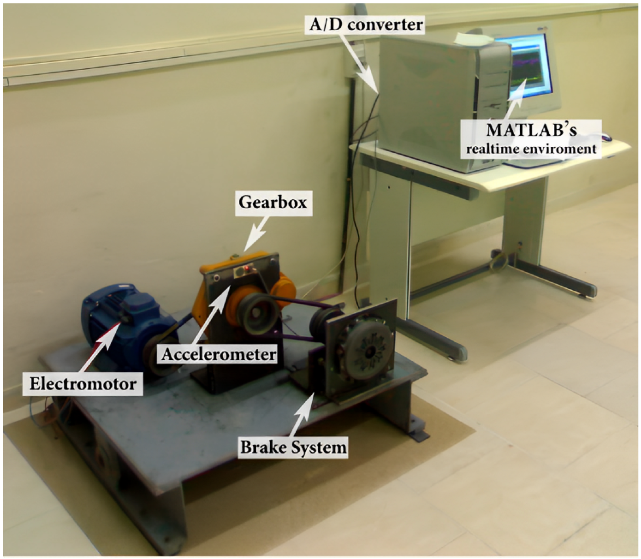
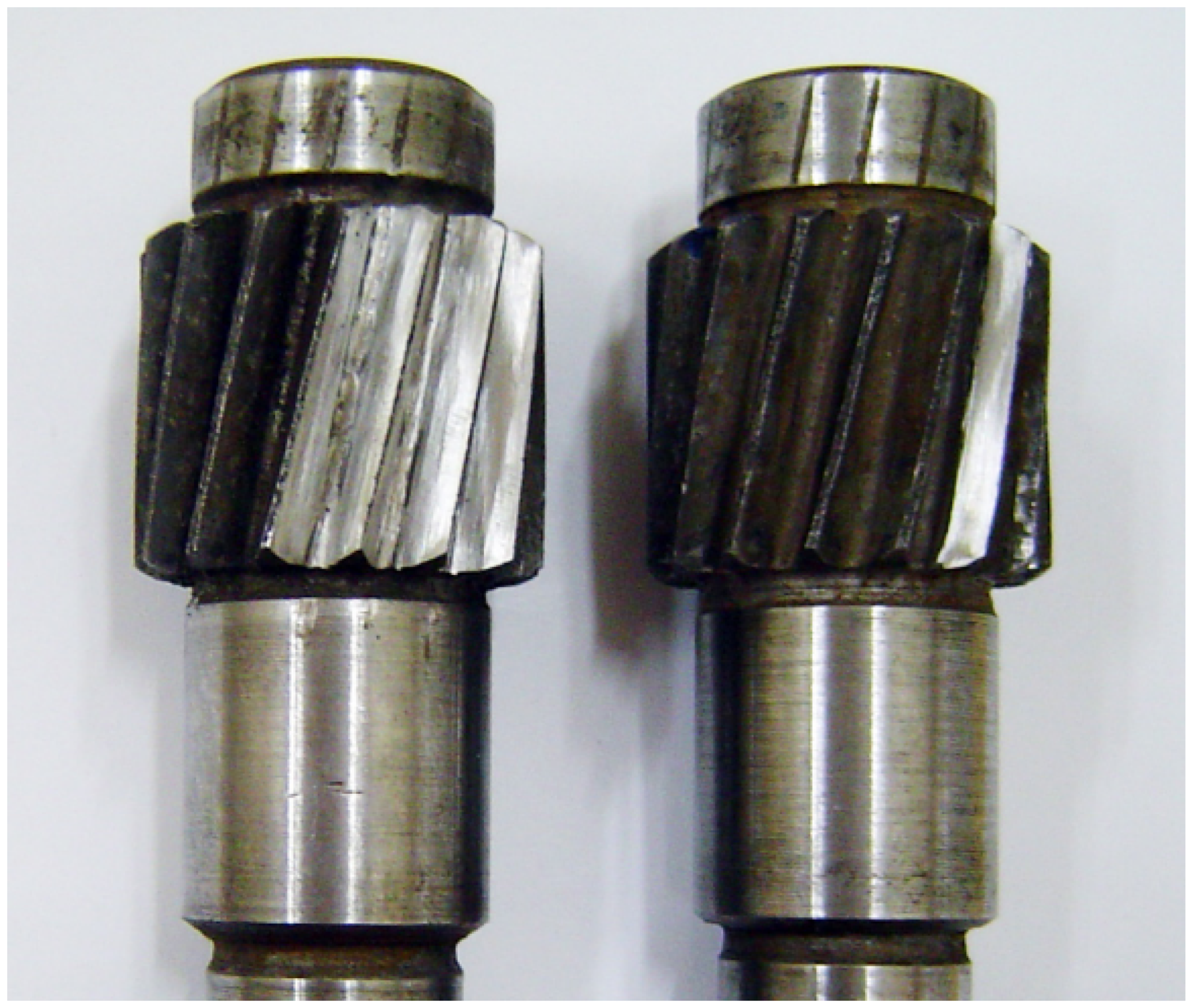
Considering that obtaining real data from industrial robot gearboxes is challenging, we used a publicly available dataset from reference [28] for this study. The dataset was collected from an experimental setup of a real industrial gearbox, simulating the working conditions of the gearbox, and records vibration signals under various typical operating conditions. It comprehensively captures the vibration characteristics induced by gear faults. The data include radial vibration signals from three different gear conditions in the gearbox setup: healthy teeth of helical gears, a single tooth gap, and three worn teeth, as shown in Figure 4 and Figure 5. Because the fault types and vibration characteristics of this dataset closely resemble common fault modes in industrial robot gearboxes, it holds significant research reference value. The data acquisition system has a sampling frequency of 10 kHz, with each collection lasting 10 s, providing high-resolution dynamic signals that help capture transient vibration features during fault occurrences. The test gearbox operates at a speed of 1420 rpm, with the small gear having 15 teeth and the large gear having 110 teeth, and a meshing frequency of 355 Hz, which accurately reflects the vibration characteristics during the gear meshing process.

In this study, we conducted fault diagnosis analysis on an industrial gearbox under three conditions: healthy teeth, chipped teeth, and worn teeth. The dataset consists of 1092 triaxial vibration signal samples, evenly distributed across the three conditions with 364 samples per category, ensuring class balance and facilitating fair learning of each fault mode by the model. Each sample contains 274 data points, representing a segment of vibration signals collected from an industrial gearbox operating at 1420 RPM, covering part of a 10 s sampling period. This ensures that the dynamic characteristics of faults are captured. The signals were acquired using industrial-grade accelerometers (Analog Devices ADXL210JQC, sensitivity 100 mV/g) and a high-precision ADC (Advantech PCI-1710, 12-bit resolution, sampling rate 100 kS/s). The signals were stored in MATLAB 2016 as voltage data after preprocessing to remove baseline drift. The theoretical gear meshing frequency (GMF) of the gearbox is 355 Hz, while the actual peak frequency obtained through FFT analysis is 365 Hz. The dataset was split into training, validation, and testing sets at a 6:2:2 ratio, with each category—including healthy teeth, chipped teeth, and worn teeth—represented in each subset, ensuring high industrial relevance. Unlike synthetic datasets, this dataset is derived from real-world industrial experiments, reflecting the nonlinear and complex nature of vibration signals. It provides researchers with reliable data for fault feature extraction and the training and validation of machine learning models. The specific data distribution and sample details are shown in

Table 2. Distribution of experimental sample dataset.

Gearbox Condition	Speed (rpm)	Sample Count	Sample Length	Label
Healthy Tooth	1420	364	274	0
Tooth Gap	1420	364	274	1
Worn Teeth	1420	364	274	2

.

3.3.2. Data Preprocessing

This study applied a logarithmic (Log) nonlinear transformation function to the vibration signals of industrial gearboxes, combined with signal standardization. The primary motivation for this approach lies in the characteristics of vibration signals, which often exhibit large amplitude peaks and small background fluctuations. Directly processing the raw signal may cause the model to overly focus on high-amplitude features while neglecting subtle yet important variations. By applying the Log transformation, the dynamic range of the signal is compressed, reducing the influence of large amplitudes while enhancing the relative importance of small-amplitude features, thus achieving a more balanced feature distribution. Moreover, the Log transformation suppresses noise signals to some extent, improving the signal-to-noise ratio. However, it is important to note that the Log transformation itself is not a normalization process—it only adjusts the amplitude proportions of the signal without scaling it to a specific range (e.g., [0, 1] or [−1, 1]). To eliminate differences in magnitude between signals, we further standardized the Log-transformed signal to ensure a more consistent feature distribution. The results of applying the Log nonlinear transform to the healthy tooth, tooth gap, and worn teeth cases are shown in Figure 6.

Figure 7 presents a comparison of the peak values between the raw signal and the logarithmically transformed signal for worn teeth. The raw signal exhibits significant amplitude fluctuations, with widely scattered peak distributions and irregular intervals between peaks, potentially reflecting the nonlinear characteristics of the wear process. In contrast, the logarithmically transformed signal demonstrates compressed amplitude ranges, smoother waveforms, and significantly reduced peak fluctuations. The logarithmic transformation highlights low-amplitude fluctuations and long-term trends within the signal, making subtle changes more prominent while smoothing out some of the sharper peak characteristics. By comparing the peak values of the two signals, it is evident that logarithmic transformation not only mitigates extreme fluctuations but also enhances the visibility of minor variations. This improvement facilitates the identification of low-amplitude changes in wear monitoring. In summary, logarithmic transformation plays a crucial role in signal processing by smoothing waveforms and emphasizing low-frequency components, thereby enabling more accurate monitoring of early changes in worn teeth.

3.3.3. MS-EMD Decomposition and Feature Selection

Compared with traditional signal decomposition techniques such as wavelet transform, empirical wavelet transform (EWT), and variational mode decomposition (VMD), MS-EMD offers significant advantages. While wavelet transform is widely used in time–frequency analysis, it requires the predefinition of a mother wavelet function, limiting its flexibility, and its performance deteriorates when dealing with high-noise signals [29]. EWT and VMD improve decomposition efficiency and noise resistance but are sensitive to parameter initialization and exhibit higher computational complexity [30,31,32]. MS-EMD, on the other hand, achieves adaptive processing of non-stationary signals through multi-scale decomposition without requiring predefined basis functions or complex parameter tuning. This makes it particularly well suited for industrial signal analysis under complex operating conditions.

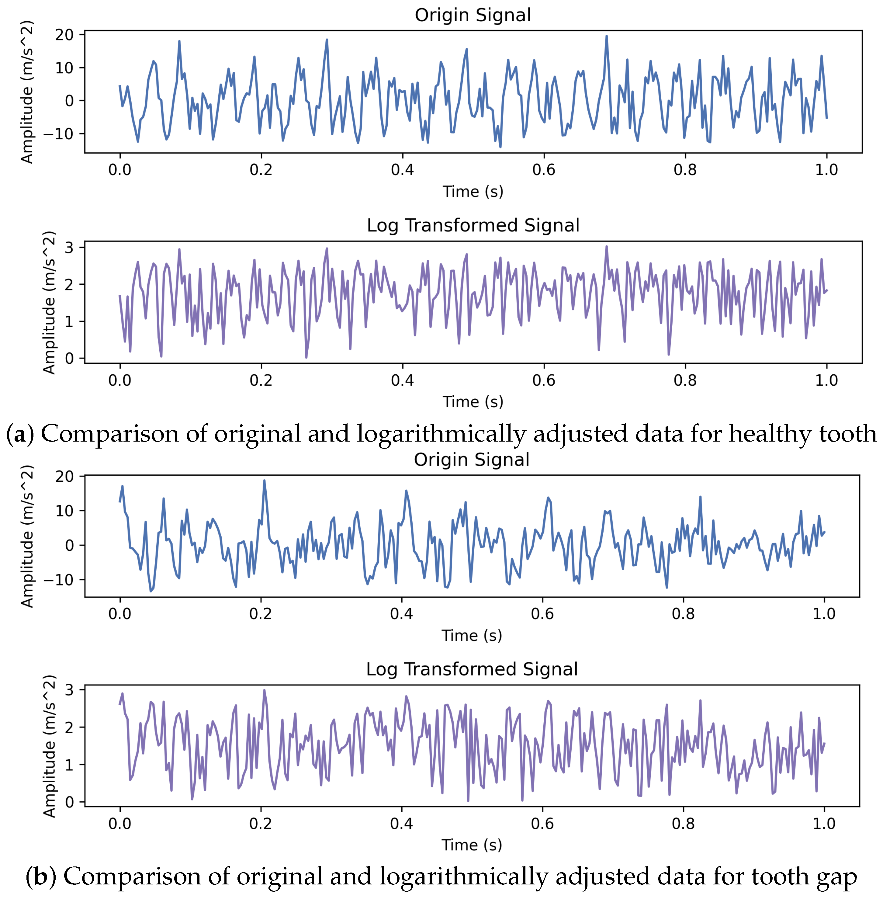
In this subsection, we show how the tooth gap fault data are handled in the MS-EMD decomposition and feature filtering steps. First, the log-transformed tooth gap signal is preprocessed using a low-pass filter, whose cutoff and order are adjusted dynamically based on the sampling rate and chosen down-sampling factors. This filter not only suppresses aliasing but also keeps the low-frequency content intact, providing a clean input for the multi-scale decomposition.

Next, the signal is down-sampled with factors of two, four, and eight to create multiple sequences at different time resolutions; the down-sampling factors of two, four, and eight were chosen because they follow a multiplicative relationship, allowing for a gradual reduction in temporal resolution to extract different signal characteristics sequentially. These factors are simple and efficient as they align with the binary nature of data processing. They are widely applied in fields such as signal processing and wavelet analysis, where their incremental pattern has been proven to effectively balance precision and efficiency. When changing the down-sampling factor reveals features in the high-, mid-, and low-frequency bands, larger factors yield lower time resolution and capture global trends, while smaller factors retain finer details for local analysis. The down-sampling process not only alters the time resolution of the signal but also reduces its amplitude to some extent. By applying down-sampling, local details of the signal are smoothed out, and the fluctuation amplitude gradually decreases. As a result, the signal exhibits a smoother variation trend at lower time resolutions. This process helps EMD to better identify low-frequency components of the signal and reduces the impact of noise on the decomposition results. The core of EMD lies in decomposing the signal into multiple intrinsic mode functions (IMFs), with each IMF representing a specific frequency component of the signal. Smaller amplitude fluctuations mitigate the interference of high-frequency noise during the EMD decomposition process. This ensures that the extracted IMFs better capture the essential characteristics of the signal rather than being overly influenced by transient peaks and local noise. The resulting signals after down-sampling by two, four, and eight are shown in Figure 8, illustrating how the tooth gap fault signature evolves across scales. These scaled signals enrich the information available for the subsequent EMD decomposition.

These multi-scale signals offer detailed input for the subsequent EMD process, enabling thorough analysis across various frequency ranges and temporal scales. This enables more precise extraction of key features of the tooth gap fault. After generating the multi-scale signals, we applied empirical mode decomposition to each scale separately. EMD works by iteratively peeling off the signal’s own oscillation patterns, so you do not need to define any wave shapes in advance. This flexibility makes it easier to uncover how the signal’s behavior changes over time. By performing EMD decomposition on signals at different scales, we can capture detailed information from various frequency bands. At higher time resolution, EMD extracts subtle changes and local vibration patterns, while at a lower time resolution, EMD is more effective at capturing the global trends and low-frequency components of the signal, offering a macro perspective on fault evolution. Figure 9 shows the EMD decomposition results of the tooth gap fault data at different down-sampling factors. The differences in frequency and time resolution of signals at various scales can be clearly observed, further validating the effectiveness of the MS-EMD method in multi-scale signal analysis.

Down-sampling factors of two, four, and eight reveal different characteristics of the signal at various time scales. Considering the signal’s frequency distribution, a down-sampling of two retains more high-frequency components, making it suitable for analyzing rapid variations and subtle fluctuations in the signal. In contrast, a down-sampling of four focuses on extracting mid-frequency features, while a down-sampling of eight emphasizes low-frequency components and long-term trends. This layered approach provides a comprehensive view of the signal across high-, mid-, and low-frequency bands. Larger down-sampling factors, such as four and eight, effectively suppress the high-frequency components of the signal, reducing amplitude fluctuations and enhancing the extraction of low-frequency information. This aids EMD in decomposing the signal by isolating stable and representative low-frequency components while mitigating the interference of high-frequency noise. As the down-sampling factor increases, the time resolution of the signal decreases, details are smoothed out, and the overall signal becomes more uniform. For fault signals like those associated with gear tooth defects, such down-sampling emphasizes the long-term trends and low-frequency variations in the signal. This results in clearer decomposition outcomes for EMD, facilitating the identification of fault characteristics. By selecting appropriate down-sampling factors, such as four or eight, unnecessary details can be minimized, allowing EMD to focus on the signal’s primary trends and extract more representative features, thereby providing more reliable information for fault diagnosis.

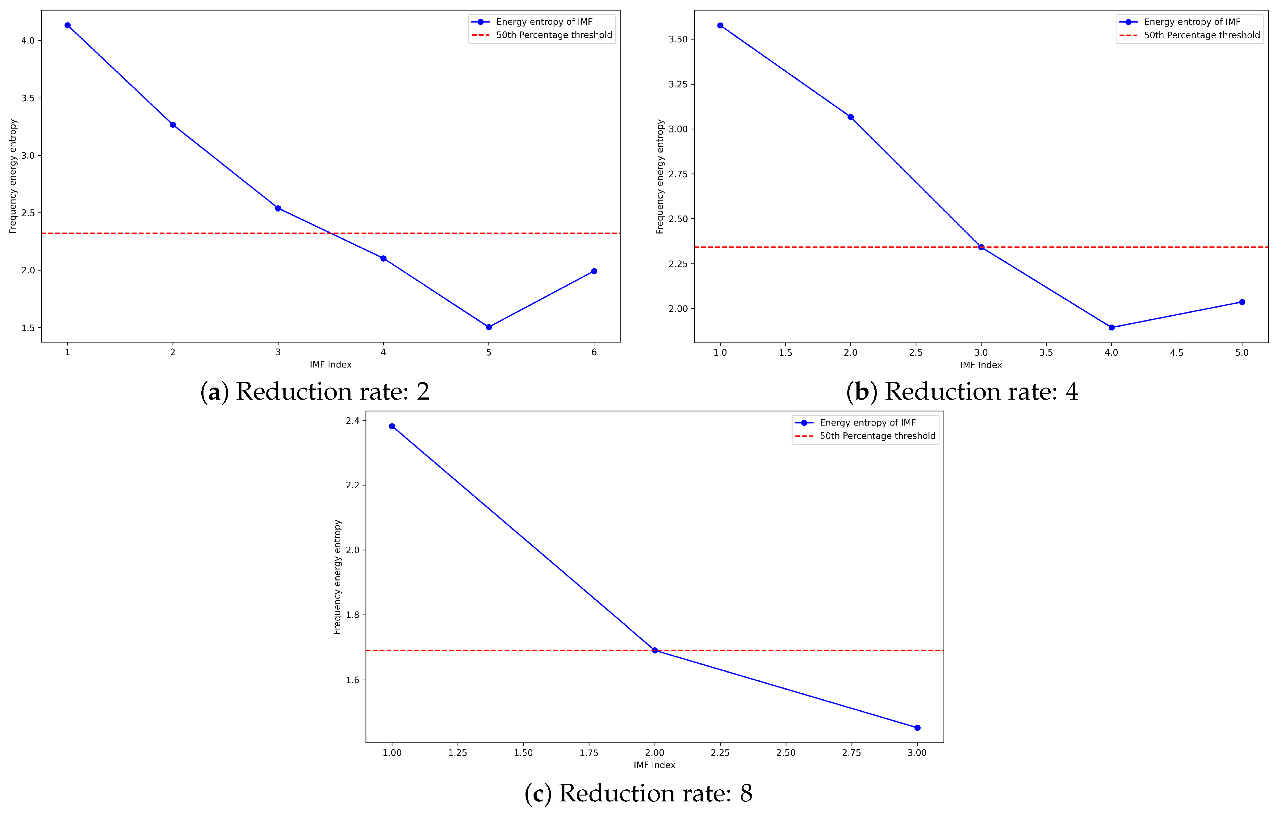
To select the key IMFs containing fault information, we use the frequency energy entropy method to evaluate the energy distribution of each IMF (the specific calculation is given in Formula (11)). By setting a 50% energy threshold, only the IMFs with energy entropy below this threshold are retained, thus removing noise and irrelevant high-frequency information while highlighting low-frequency fault features.

$$\begin{array}{c}H=-{\displaystyle \sum _{i=1}^n}{P}_{i}log\left(P_i\right)\end{array}$$

(11)

To filter the IMFs, in this study, a 50% frequency energy entropy threshold was empirically set as the criterion for determining key intrinsic mode functions (IMFs) [29]. The 50% energy threshold serves as a balancing strategy that retains most of the useful information in the signal while effectively filtering out secondary modes, thus preventing the model from becoming overly complex due to redundant features. Only IMFs with energy entropy below this threshold are kept, as these components are typically concentrated in the low-frequency range and contain the primary fault characteristics. In contrast, IMFs with higher energy entropy are generally random noise or high-frequency irrelevant information. The selection of the 50% energy entropy threshold is not arbitrary but rather a balanced strategy supported by theoretical analysis and experimental validation. Energy entropy, as an indicator of signal complexity and randomness, reflects the energy distribution of the signal across different frequency bands. By choosing an appropriate threshold, it is possible to retain the main features of the signal while effectively filtering out high-frequency noise. The threshold setting must strike a balance between retaining meaningful features and eliminating noise, avoiding excessive information loss or noise interference. The 50% energy entropy threshold can be explained from several perspectives. First, it is a commonly used empirical choice that aims to retain most of the useful information while efficiently filtering out noise. Low-frequency components usually contain the signal’s main features, while high-frequency parts tend to include noise or irrelevant components. By selecting a 50% threshold, key low-frequency information in the signal is preserved, while high-frequency noise is suppressed, reducing interference in signal analysis. Additionally, experimental results indicate that the 50% energy entropy threshold provides good decomposition performance for most signals. When compared with other thresholds (e.g., 30%, 40%, 60%), the IMFs selected with the 50% threshold typically highlight the fault characteristics of the signal and reduce irrelevant information, improving the accuracy of subsequent fault diagnosis models. A threshold that is too low (e.g., 30%) may retain too many IMFs, including significant high-frequency noise, which increases computational complexity and affects subsequent analysis. A threshold that is too high (e.g., 70%) may better suppress noise but could also lose important details of the signal. The 50% threshold effectively balances information retention and the removal of redundant information, preventing overcomplication while preserving essential details. Moreover, the 50% energy entropy threshold significantly improves the signal reconstruction quality. The filtered IMFs are smooth, with noticeable noise suppression. Compared with other thresholds, the IMFs obtained with the 50% threshold retain the low-frequency information of the signal better while reducing high-frequency noise interference, providing clearer and more reliable input data for subsequent feature extraction and fault diagnosis.

In

Table 3. Reconstruction errors of different threshold signals.

Thresholds (%)	MSE	RMSE
30%	0.034	0.184
40%	0.028	0.167
50%	0.022	0.148
60%	0.025	0.158

, we present the signal reconstruction errors under different energy entropy thresholds (30%, 40%, 50%, 60%), including mean squared error (MSE) and root mean square error (RMSE). By comparing the results for different thresholds, it is evident that the 50% energy entropy threshold performs the best in signal reconstruction, exhibiting the lowest MSE and RMSE values. This indicates that the 50% threshold can effectively retain the key signal features while suppressing high-frequency noise, ensuring the accurate extraction of the main characteristics of the signal. On the other hand, lower thresholds (such as 30% and 40%) retain too much high-frequency noise, leading to higher reconstruction errors. Higher thresholds (like 60%) may remove more noise but also result in the loss of important low-frequency information, causing a decline in reconstruction performance. Therefore, the 50% energy entropy threshold strikes a good balance between noise suppression and feature retention, providing the optimal signal reconstruction performance. This makes it a reliable data source for subsequent fault diagnosis and feature extraction.

During the filtering process, the frequency energy entropy distribution under different down-sampling factors is shown in Figure 10. From the figure, it can be seen that as the down-sampling factor increases, the frequency energy entropy distribution of the IMFs exhibits a certain regularity. For instance, larger down-sampling factors correspond to IMFs in lower frequency ranges, which usually have lower energy entropy, indicating that the signal energy is more concentrated. On the other hand, smaller down-sampling factors retain more high-frequency components, with their corresponding IMF energy entropy distribution being more dispersed. Finally, the selected IMFs are re-constructed into a new signal, a process that not only effectively reduces irrelevant noise in the data but also enhances the clarity of the fault feature signals, providing more reliable and clear input data for the subsequent 1D CNN-BiGRU fault diagnosis model.

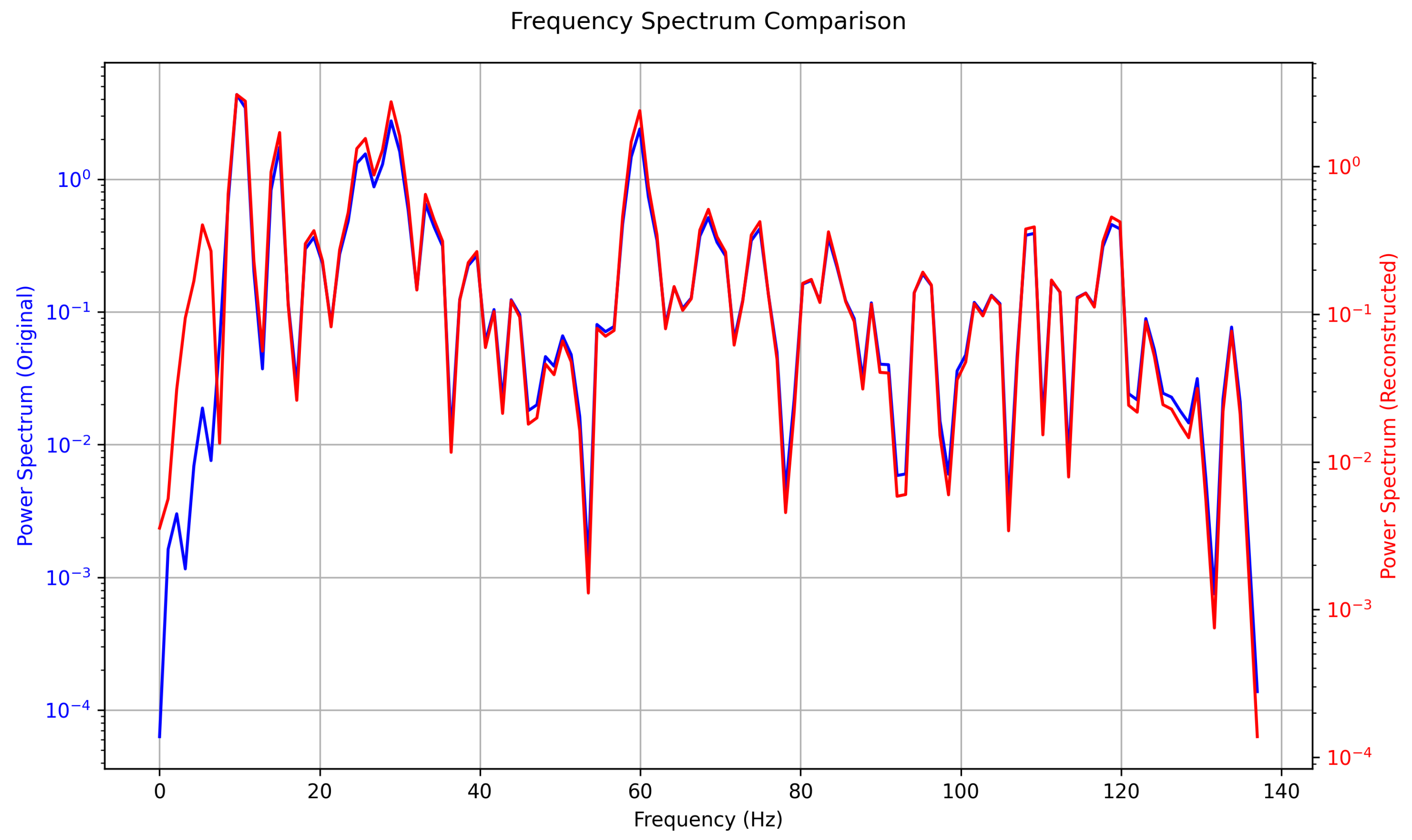
From the spectral comparison in Figure 11, several key features can be observed. The frequency spectra of the original signal and the reconstructed signal show significant differences in the 0–10 Hz range. This could be because the low-frequency energy is primarily contributed by noise or other non-characteristic components in the original signal. The MS-EMD decomposition process exhibits good noise suppression capabilities in the low-frequency band, effectively removing irrelevant low-frequency noise in the reconstructed signal. In the 10–140 Hz frequency range, the spectra of the original and reconstructed signals are almost identical, indicating that the MS-EMD method can accurately extract frequency features related to the fault, with no significant loss of key information during the reconstruction process. This result demonstrates that MS-EMD not only extracts fault characteristic signals but also preserves the high fidelity of the signal, ensuring that the reconstructed signal retains the primary dynamic features of the original signal in its spectrum.

3.4. Experimental Results

To thoroughly evaluate the proposed MS-EMD and 1D CNN-BiGRU fault diagnosis model, a set of detailed experiments was conducted. The training process was analyzed by tracking accuracy and loss trends, and 5-fold cross-validation was applied to ensure consistent and reliable outcomes. Additionally, the model’s ability to classify different fault types was assessed using performance measures like confusion matrix, precision, recall, and F1-score. In the comparison experiments, five classical algorithms, namely CNN, 1D Transformer, GRU, ResNet-18, and 1D CNN-GRU, were selected for a comprehensive comparison, as shown in

Table 4. Network architectures of different comparison methods.

Model	Network Structure
CNN	Convolutional Layer—Pooling Layer—Convolutional Layer—Pooling Layer—Fully Connected Layer
1D Transformer	Input Embedding Layer—Multi-Head Self-Attention Layer—Feedforward Neural Network—Output Layer
GRU	Input Layer—GRU Units—Fully Connected Layer—Output Layer
ResNet-18	Convolutional Layer—Residual Block—Residual Block—Fully Connected Layer—Output Layer
1D CNN-GRU	1D Convolutional Layer—GRU Layer—Fully Connected Layer—Output Layer

. These methods are representative: CNN is typical architectures of traditional convolutional neural networks, excelling at local feature extraction but lacking in temporal modeling ability. The 1D Transformer utilizes the self-attention mechanism to capture global dependencies within the input sequence, making it particularly well suited for handling complex patterns in long time-series data. It excels at capturing global features, which is its key strength. However, it comes with the tradeoff of higher computational complexity and slower inference speed. Despite these drawbacks, its performance on complex datasets generally surpasses that of traditional convolutional networks, making it a powerful tool for tasks requiring the modeling of long-range dependencies and intricate data patterns. GRU focuses on dynamic evolution features of signals, demonstrating strong temporal modeling capabilities. ResNet-18, with its residual network structure, addresses the difficulty of training deep networks and has a strong generalization ability. The 1D CNN-GRU approach combines the ability of convolutional networks to capture features with the GRU’s capacity for handling time-based patterns. However, it falls short in fully capturing information from both past and future sequences compared with BiGRU. The proposed MS-EMD-1D CNN-BiGRU model leverages multi-scale decomposition for adaptive feature extraction, paired with the strengths of 1D CNN-BiGRU in identifying local features and understanding patterns from both directions. This method achieved better accuracy and reliability under challenging conditions. Experimental comparisons highlight notable improvements in performance, showcasing its practical value and offering insights for further enhancements in fault detection for industrial robots.

3.4.1. Training Process Analysis

As shown in Figure 12, this paper presents the comparison results of the MS-EMD-1D CNN-BiGRU model with five classical models, including CNN [33], 1D Transformer [34], GRU [35], ResNet-18 [36], and 1D CNN-GRU [37], in terms of accuracy and loss values. The results indicate that the MS-EMD-1D CNN-BiGRU model demonstrates significant superiority during the training process. Its accuracy increases rapidly, eventually reaching the highest value, while the loss value decreases steadily and quickly, fully validating the model’s efficiency and reliability in complex fault diagnosis tasks.

From the accuracy curve in Figure 12a, the MS-EMD-1D CNN-BiGRU model effectively enhances the quality of signal feature extraction through multi-scale decomposition. Combined with the local feature extraction capability of 1D CNN and the global temporal modeling ability of BiGRU, the model is able to effectively capture key feature information in bearing fault signals, enabling fast convergence and higher accuracy. In contrast, traditional convolutional networks such as CNN have certain advantages in spatial feature extraction but are limited by their inability to process temporal information, which restricts their classification performance. The 1D Transformer effectively captures global temporal dependencies using the self-attention mechanism, making it especially suitable for handling long-sequence signals. However, its computational complexity is relatively high, and the inference speed is slower, which may make it less suitable for tasks requiring high real-time performance. The GRU model performs well in handling temporal information but lacks the capability to extract spatial features, limiting its overall performance. Although ResNet-18 has strong feature extraction ability through its deep architecture, its higher model complexity affects its adaptability to small sample data. The 1D CNN-GRU model, to some extent, integrates spatial and temporal features, but its feature fusion strategy is not as effective as that of the MS-EMD-1D CNN-BiGRU model, leading to slightly worse performance.

From the loss curve in Figure 12b, it can be observed that the MS-EMD-1D CNN-BiGRU model exhibits the steepest and smoothest loss value decrease, indicating that its optimization process is stable and efficient, with excellent convergence performance. The loss value decrease in other comparative models is slower, with varying degrees of fluctuation, reflecting their shortcomings in feature extraction and parameter optimization.

In conclusion, the superiority of the MS-EMD-1D CNN-BiGRU model lies in its multi-scale decomposition method, which effectively enhances the signal’s feature representation capabilities. The combination of 1D CNN and BiGRU enables deep integration of spatial and temporal features, making it superior to the comparison models in both accuracy and loss value. The robustness and efficiency demonstrated by this model under complex working conditions provide strong technical support for intelligent fault diagnosis of industrial equipment.

3.4.2. Multi-Metric Evaluation of Model Performance

Table 5. Multi-metric evaluation of model performance.

Method	Avg. Accuracy (%)	Healthy Precision (%)	Healthy Recall (%)	Healthy F1 (%)	Crack Precision (%)	Crack Recall (%)	Crack F1 (%)	Worn Precision (%)	Worn Recall (%)	Worn F1 (%)	5-Fold CV (%)
CNN	96.34	96.10	96.20	96.15	96.30	96.40	96.35	96.60	96.50	96.55	$96.34\pm 1.12$
1D Transformer	99.21	98.95	99.01	98.97	99.15	99.20	99.10	99.25	99.23	99.20	$99.21\pm 1.56$
GRU	88.83	88.50	88.60	88.55	88.70	88.80	88.75	89.30	89.20	89.25	$88.83\pm 2.05$
ResNet-18	89.92	89.60	89.50	89.55	89.80	90.00	89.90	90.20	90.30	90.25	$89.92\pm 1.87$
1D CNN-GRU	99.36	99.20	99.30	99.25	99.40	99.50	99.45	99.50	99.40	99.45	$99.36\pm 0.78$
MS-EMD-1D CNN-BiGRU	99.58	99.60	99.60	99.60	99.50	99.60	99.55	99.60	99.50	99.55	$99.58\pm 0.65$

presents a more detailed classification performance of different methods in the fault diagnosis task, including overall average accuracy, as well as precision, recall, F1-score, and 5-fold cross-validation results for the three fault types: healthy gears, gear tooth cracks, and worn gears. These data not only reflect the overall performance of the models but also reveal their classification ability for each fault category.

The CNN method achieved an average accuracy of 96.34%, with F1-scores for healthy gears, gear tooth cracks, and worn gears being 96.15%, 96.35%, and 96.55%, respectively, indicating its ability to extract fault features to some extent. However, its performance is limited in complex fault patterns due to its weak capability in handling temporal information.

The 1D Transformer method optimized global temporal modeling, improving the average accuracy to 99.21%. The F1-scores for healthy gears, gear tooth cracks, and worn gears reached 98.97%, 99.1%, and 99.2%, respectively, with a 5-fold cross-validation fluctuation of ±1.56, demonstrating high classification performance and good stability.

The GRU method introduced a temporal modeling mechanism, with F1-scores for healthy gears, gear tooth cracks, and worn gears being 88.55%, 88.75%, and 89.25%, respectively. However, due to its lack of spatial feature extraction ability, the average accuracy was only 88.83%, and the 5-fold cross-validation fluctuation was relatively large (±2.05), reflecting insufficient performance and stability.

ResNet-18 improved spatial feature extraction through a deep convolutional network, achieving an average accuracy of 89.92%. However, its performance across the fault types was still lower than that of more complex hybrid models.

The 1D CNN-GRU method combined CNN’s spatial feature extraction ability with GRU’s temporal modeling ability, achieving an average accuracy of 99.36%. The F1-scores for healthy gears, gear tooth cracks, and worn gears were 99.25%, 99.45%, and 99.45%, respectively, with a reduced 5-fold cross-validation fluctuation of ±0.78, showing a good balance of performance.

The proposed MS-EMD-1D CNN-BiGRU method outperformed all other methods in every metric, with an average accuracy of 99.58%. The F1-scores for healthy gears, gear tooth cracks, and worn gears were 99.6%, 99.55%, and 99.55%, respectively. Furthermore, the 5-fold cross-validation fluctuation was only ±0.65, indicating the method’s high robustness under different data partition conditions. By extracting key feature signals through MS-EMD and combining CNN and BiGRU for spatial and temporal feature modeling, this method not only leads in overall performance but also demonstrates exceptional classification accuracy across different fault categories, fully showcasing its strong adaptability in complex fault diagnosis tasks.

3.4.3. Visual Analysis of Confusion Matrix

As shown in Figure 13, the confusion matrix provides a visual analysis of the prediction results of the six models on the test set, allowing for a direct comparison of their performance in the fault classification task. The MS-EMD-1D CNN-BiGRU model proposed in this study performs the best, achieving an average accuracy of 99.58% with only four misclassifications, securing the top position. The 1D CNN-GRU model follows closely with an accuracy of 99.36% and seven misclassifications.

In terms of weaker-performing models, the traditional CNN and GRU models have accuracies of 96.34% and 88.83%, respectively, with 32 and 89 misclassifications, highlighting significant shortcomings. Specifically, the GRU model, due to its insufficient local feature extraction capability and reliance solely on temporal modeling, has limited classification ability for complex fault signals. Additionally, while the ResNet-18 model possesses strong deep feature extraction capabilities, its large parameter size makes it susceptible to small sample noise, resulting in an accuracy of 89.92% and 82 misclassifications.

It is noteworthy that the MS-EMD-1D CNN-BiGRU model has the fewest misclassifications, which fully validates its ability to efficiently integrate spatial and temporal features by extracting multi-scale features using MS-EMD and combining 1D CNN and BiGRU. This characteristic enables it to excel in capturing key fault features under complex operating conditions. Meanwhile, compared with other models, the 1D CNN-GRU models, with their stronger local feature extraction abilities, show relatively stable performance but still fall short in global temporal dependency modeling compared with MS-EMD-1D CNN-BiGRU.

In summary, the excellent performance of the MS-EMD-1D CNN-BiGRU model is reflected not only in its high accuracy but also in its effective suppression of misclassifications, demonstrating remarkable robustness and reliability. This performance advantage makes the model highly suitable for wide application in industrial fault diagnosis.

3.4.4. T-SNE Clustering Visualization Analysis

Figure 14 illustrates the visualization of the feature clustering process of the MS-EMD-1D CNN-BiGRU model at different network layers using T-SNE [38]. T-SNE is a dimensionality reduction technique commonly used to visualize high-dimensional data in 2D space. In this context, it helps to reveal the separability and clustering patterns of features learned by different layers of the model, offering insights into how the network transforms raw input data into meaningful representations. This figure provides an intuitive observation of the model’s step-by-step evolution in extracting and optimizing gearbox vibration signal features.

At the raw data layer, the feature distribution is quite chaotic, with unclear boundaries between different fault categories and noticeable overlap between feature points. This reflects the low discriminability of the original gearbox vibration signal, making it difficult to directly use for classification tasks. However, as the data are processed layer-by-layer through the convolution layers (Conv1, Conv2, and Conv3), local features are gradually extracted and optimized. Specifically, at the Conv1 layer, the model begins to extract preliminary edge features, and the feature distribution converges compared with the original signal, though there is still significant class overlap. At the Conv2 layer, the features begin to show more structure, with improved class separation. By the Conv3 layer, the local features are further enhanced, and the clustering effect is significantly improved, with clearer separation between categories and more compact feature points.

Subsequently, the BiGRU layer introduces bidirectional temporal modeling, which fully combines the sequential dependencies of the data from both directions. This enhances the global consistency and temporal correlation of the features. At this stage, both intra-class compactness and inter-class separation are significantly improved, and the class boundaries start to become clearer. This shows that BiGRU not only effectively complements the convolution layers in global modeling but also enhances the ability to capture complex temporal information.

Finally, at the output layer, the deep fusion of convolutional feature extraction and BiGRU temporal modeling results in high-level features that exhibit strong discriminability. The feature clusters of different fault categories are almost completely separated. This highly optimized feature representation indicates that the MS-EMD-1D CNN-BiGRU model can fully exploit the deep information of the gearbox vibration signal and convert it into highly distinguishable features.

In summary, the T-SNE visualization results in Figure 14 visually confirm the stepwise optimization process of the MS-EMD-1D CNN-BiGRU model, from local feature extraction to global temporal modeling. It comprehensively demonstrates the model’s superiority in feature extraction and class distinction, providing strong support for efficient fault diagnosis under complex operating conditions.

3.5. Comparative Analysis of Different Datasets

3.5.1. Paderborn Datasets

The Paderborn dataset, provided by Germany’s Paderborn University, is a high-quality rolling bearing fault dataset widely used in the fault diagnosis field. This dataset includes multiple fault states such as normal operation, outer ring faults, inner ring faults, and rolling element faults, as shown in

Table 6. Paderborn select data categories.

Fault Type	Rotational Speed (rpm)	Load (Nm)	Sampling Frequency (kHz)	Condition Description	Label
No Fault	1500	0	64	Low-speed, light-load	0
Rolling Element Fault	1500	1	64	Low-speed, medium-load	1
Inner Ring Fault	1500	2	64	Low-speed, heavy-load	2
Outer Ring Fault	2000	1	64	Medium-speed, medium-load	3
Compound Fault	2500	2	64	High-speed, heavy-load	4
Rolling Element Fault	2500	0	64	High-speed, light-load	5

. Vibration signals were collected under varying rotational speeds (1500 rpm, 2000 rpm, 2500 rpm) and loads (0 Nm, 1 Nm, 2 Nm), featuring a high sampling rate (64 kHz) and diverse operating conditions.

In this study, experiments were conducted using multiple combinations of speeds and loads, covering typical industrial scenarios ranging from low-speed light-load to high-speed heavy-load conditions. The objective was to thoroughly evaluate the model’s performance in feature extraction, adaptability to complex conditions, and noise suppression. Particularly under high-speed and high-load conditions, where signal characteristics become more intricate, the model’s robustness and anti-interference capabilities face greater challenges. This provides more compelling validation for the model’s application in real-world industrial environments.

3.5.2. Multi-Metric Evaluation of Model Performance

Table 7. Test results of different evaluation metrics on the Paderborn dataset.

Method	Average Accuracy (%)	Accuracy (%)	Recall (%)	F1-Score (%)	5-Fold Cross-Validation (%)
CNN	93.52	93.56	93.63	93.52	93.5 ± 3.0
1D Transformer	98.86	98.91	98.93	98.85	98.8 ± 2.8
GRU	92.52	92.36	92.71	92.51	92.5 ± 3.2
ResNet-18	95.66	95.23	96.12	95.64	95.6 ± 2.5
1D CNN-GRU	99.13	99.06	98.42	99.12	98.2 ± 1.7
MS-EMD-1D CNN-BiGRU	99.32	99.41	99.23	99.34	99.3 ± 1.5

shows the test results of different methods on the Paderborn dataset, including average accuracy, precision, recall, F1-score, and the variation of 5-fold cross-validation. The test set used during the testing process includes six uniformly distributed fault category samples. By testing the results of these samples, it is possible to clearly observe the performance differences of each method under different experimental conditions, as well as their adaptability in complex working environments.

In traditional methods, CNN achieves an average accuracy of 93.52%, with stable performance. However, it still faces limitations in capturing temporal information and adapting to complex conditions. GRU performs relatively poorly, with an accuracy of 92.52%, mainly due to its weakness in capturing local spatial features. In comparison, ResNet-18 performs excellently, achieving an accuracy of 95.66% and a cross-validation variation of ±2.5, demonstrating strong stability and robustness. The 1D CNN-GRU method combines the advantages of CNN and GRU, reaching an accuracy of 99.13%, close to ResNet-18, but still has room for improvement under complex conditions. The MS-EMD-1D CNN-BiGRU model, by incorporating multi-component signal decomposition and bidirectional GRU, demonstrates excellent feature extraction and temporal modeling abilities under complex conditions, achieving an accuracy of 99.32%, with superior performance across various metrics.

In conclusion, the Paderborn dataset provides an effective platform for initial model validation. However, as operating conditions become more complex (such as high-speed, heavy-load, and compound faults), a more comprehensive evaluation of the model’s performance can be performed, especially regarding its potential and reliability in real industrial applications. Therefore, the experimental design of this study is closer to real industrial environments, laying a solid foundation for further industrial applications.

3.5.3. Visual Analysis of Different T-SNE Models

Figure 15 shows the T-SNE visualization of feature clustering results for different methods on the Paderborn dataset, which intuitively reflects the differences in their performance for feature extraction and classification tasks.

The T-SNE results for the CNN method indicate that while there is some degree of separation in the feature clusters, the boundaries between categories remain unclear. This is particularly evident under complex conditions (such as high load and high speed), where there is still significant overlap in the feature clusters between categories. This suggests that CNN struggles with capturing sequential information in such dynamic conditions, which impacts classification performance. However, in cases of complex load and speed variations, the boundaries between categories are still not very distinct, with noticeable confusion under low-speed and high-load conditions. The T-SNE results for the GRU model show relatively poor clustering, with blurred category boundaries and significant overlap. While GRU has advantages in handling sequential data, its ability to capture local spatial features is weak, making it difficult to extract distinguishable features in complex conditions. Compared with CNN, GRU performs less effectively. The ResNet-18 model stands out with clear feature clustering and strong category separation in the T-SNE visualization. Its deep network structure effectively extracts more complex features, allowing it to maintain good separation between categories even in high-load and high-speed conditions, demonstrating strong robustness and stability. The 1D CNN-GRU combines the spatial feature extraction capabilities of CNN with the sequential modeling abilities of GRU. T-SNE results show exceptional feature clustering, with clear and well-separated feature distributions for different categories in the low-dimensional space. Particularly under complex, dynamic conditions, the model efficiently extracts sequential information and local features, leading to clearer category boundaries and outstanding performance in such conditions. The MS-EMD-1D CNN-BiGRU method demonstrates the best performance in T-SNE visualization, with nearly complete separation of categories and minimal overlap. This indicates that the method significantly improves feature extraction capabilities when handling complex conditions. By leveraging multi-component signal decomposition and bidirectional GRU for sequential modeling, it effectively deals with complex signals, showing high accuracy and robustness.

In summary, the T-SNE visualization in Figure 15 highlights the differences in the ability of different methods to handle feature clustering on the Paderborn dataset. While traditional methods like CNN and GRU can perform basic feature extraction, they still struggle under complex conditions. In contrast, ResNet-18 and 1D CNN-GRU show superior performance, and our MS-EMD-1D CNN-BiGRU method, with its multi-component signal decomposition and improved network structure, demonstrates high robustness and adaptability in dynamic conditions. The T-SNE results further confirm that MS-EMD-1D CNN-BiGRU not only excels at extracting features in complex industrial environments but also significantly improves classification performance, providing strong technical support and broad practical application potential for fault diagnosis in industrial settings.

3.6. Ablation Experiment

To further investigate the specific contributions of each module (MS-EMD, 1D CNN, and BiGRU) to the model’s performance and validate the rationality of the overall architecture design, we conducted ablation experiments, as detailed in

Table 8. Ablation experiment results.

Model Configuration	Dataset from [28] (%)	Paderborn Dataset (%)
MS-EMD-1D CNN-BiGRU	99.58	99.32
1D CNN-BiGRU	98.87	98.32
Single-Scale EMD-1D CNN-BiGRU	99.46	99.24
MS-EMD-1D CNN-GRU	99.53	99.29

. The experimental results in Table 8 demonstrate that the MS-EMD-1D CNN-BiGRU model achieves the best performance on both the publicly available dataset provided in [28] and the Paderborn dataset, with accuracy rates of 99.58% and 99.32%, respectively. This validates the effectiveness of the collaborative interaction among multiple modules.

When MS-EMD is removed, the accuracy drops significantly by 0.71% and 1.00%, respectively, indicating the critical role of multi-scale feature decomposition in handling non-stationary signals and noise. Substituting single-scale EMD for MS-EMD results in a slight performance decrease (0.12% and 0.08%, respectively), reflecting the advantage of multi-scale decomposition in capturing complex signal features. Furthermore, replacing BiGRU with GRU causes a marginal accuracy decline (0.05% and 0.03%, respectively), verifying the importance of BiGRU’s bidirectional temporal modeling capability in dynamic feature recognition.

Overall, the experimental results clearly demonstrate the rationality of the proposed module design and its superiority in fault diagnosis tasks.

3.7. Real-Time Performance and Computational Cost Analysis

Table 9. Computation time on the GPU and CPU for different modules.

Module	GPU Per Sample (ms)	CPU Per Sample (ms)
MS-EMD	12.5	45.3
1D CNN	4.8	20.1
BiGRU	8.2	32.7
End-to-End Time	25.5	98.1

shows the per-sample processing time for each module on the GPU and CPU. The MS-EMD module takes 12.5 ms on the GPU and 45.3 ms on the CPU, making it one of the most time-consuming steps in the process and highly dependent on hardware acceleration. The 1D CNN module has the shortest processing time on the GPU at only 4.8 ms, and it is relatively fast on the CPU as well at 20.1 ms, reflecting the high optimization of convolution operations on modern hardware. The BiGRU module takes 8.2 ms on the GPU and 32.7 ms on the CPU, indicating its complexity is between MS-EMD and 1D CNN, while still showing good performance under GPU acceleration. The end-to-end total processing time (MS-EMD + 1D CNN + BiGRU) is 25.5 ms on the GPU and 98.1 ms on the CPU. GPU acceleration significantly enhances the overall inference speed, enabling near real-time diagnostic capability at approximately 40 Hz on high-performance computing platforms, whereas the CPU performance is more suited for offline analysis.

As shown in Table 9, the model achieves a single-sample processing time of 25.5 ms on the GPU, corresponding to approximately 40 Hz. Considering typical requirements for gearbox monitoring systems, where sampling rates and fault response times are generally within the tens of milliseconds range, the reported inference time demonstrates that our method is well suited for most industrial scenarios. It enables online continuous monitoring and rapid fault detection, thereby enhancing operational safety and reliability.

It is worth noting that although the model’s single-sample inference time on GPU is 25.5 ms, and the typical industrial sampling rate is 1 kHz (i.e., one sample per millisecond), the inference speed should be understood in the context of processing data windows rather than individual samples. Typically, data are segmented into windows of fixed length, for example, 1024 samples per window. At 1 kHz sampling rate, each window corresponds to approximately one second of signal. The inference time of 25.5 ms is significantly shorter than the window duration, enabling near real-time analysis of each window and thus supporting continuous online monitoring and timely fault diagnosis in industrial applications.

Given that MS-EMD is computationally intensive—taking 45.3 ms per sample on a CPU—its direct deployment on resource-constrained edge devices may be challenging. To address this limitation and enable practical real-time monitoring in such environments, it is necessary to explore lightweight alternatives or optimizations that maintain diagnostic effectiveness while reducing computational overhead. Below, we discuss several promising approaches for achieving this balance:

Online variants of EMD: online EMD or adaptive EEMD variants can reduce computational overhead by optimizing decomposition for real-time operation, balancing performance and efficiency.

Wavelet transform or short-time Fourier transform (STFT): these time–frequency analysis methods are computationally less intensive and could serve as effective substitutes for feature extraction in edge scenarios.

Learned representations: using machine learning models, such as neural networks trained to mimic MS-EMD decomposition, can accelerate feature extraction by leveraging pre-trained architectures optimized for specific hardware.

Preprocessing techniques: dimensionality reduction or signal compression applied before MS-EMD can lower the computational requirements without significantly compromising the diagnostic accuracy.

Table 10. GPU and CPU throughput under different batch sizes.

Batch Size	GPU Throughput (Samples/s)	CPU Throughput (Samples/s)
32	1250	326
64	1400	350
128	1500	360

shows the throughput test results for different batch sizes. As the batch size increases from 32 to 128, GPU throughput rises from 1250 samples/s to 1500 samples/s, representing an improvement of approximately 20%. This indicates that larger batch sizes can better utilize the parallel processing capabilities of the GPU, although the benefits gradually diminish. In contrast, CPU throughput increases from 326 samples/s to 360 samples/s, with only about a 10% improvement, reflecting the limitations of CPUs in parallel processing. Overall, the GPU’s throughput is 3–4 times that of the CPU, further highlighting the critical role of GPU acceleration in enhancing the real-time diagnostic performance of the model.

To improve real-time performance, future research will focus on the following optimizations:

1.

Model lightweighting: exploring strategies to reduce the model’s parameter size, such as using smaller convolution kernels in 1D CNN or utilizing depthwise separable convolutions, and reducing the number of hidden units or the temporal steps in BiGRU.

2.

Hardware acceleration: enhance the model’s execution efficiency in resource-constrained environments by introducing hardware accelerators like GPUs or FPGAs.

3.

Signal decomposition simplification: optimize the MS-EMD decomposition process to reduce computational resource usage while maintaining decomposition quality.

4.

Real-time testing: conduct more comprehensive real-time tests under actual industrial conditions, evaluate the applicability of the method, and optimize the processing flow to reduce latency.

3.8. Performance Evaluation of Real-Time Processing

For the MS-EMD-1D CNN-BiGRU model, which achieves high accuracy on the public dataset [28] and the Paderborn dataset (99.58% and 99.32%, respectively), we plan to optimize the model through pruning and quantization to ensure it meets the deployment requirements for edge devices. The specific performance evaluation data can be seen in

Table 11. Accuracy and performance results under different optimization strategies.

Optimization Strategy	Public Dataset [28] Accuracy	Paderborn Dataset Accuracy	Inference Time (per Sample)	Model Size
Original Model (MS-EMD-1D CNN-BiGRU)	99.58%	99.32%	100 ms	50 MB
Pruning—20%	99.40%	99.15%	80 ms	40 MB
Pruning—50%	99.20%	98.90%	60 ms	30 MB
Quantization—8-bit (Static)	99.40%	99.10%	50 ms	25 MB
Quantization—8-bit (Dynamic)	99.30%	98.85%	45 ms	25 MB
Pruning + Quantization (20% + 8-bit)	99.25%	98.80%	40 ms	20 MB
Pruning + Quantization (50% + 8-bit)	99.10%	98.60%	35 ms	15 MB

.

Pruning: We adopt a structured pruning strategy to remove redundant convolution kernels in the CNN part and hidden units in the BiGRU layer. This is expected to reduce computation and parameter size by 20–50%. Pruning reduces computational burden and memory usage significantly, providing more efficient inference performance for edge devices. However, pruning may lead to some accuracy loss, especially when pruning is aggressive. Therefore, fine-tuning and adjustment are required to maintain model performance.

Quantization: We combine static quantization, dynamic quantization, and mixed-precision quantization techniques to compress the model’s weights and activation values to 8 bits or lower. Quantization can greatly reduce the model’s storage requirements and improve inference speed, typically achieving a 3–4× reduction in model size and a 2× or more improvement in inference speed. The quantized model demonstrates significant advantages on edge devices, particularly in environments with limited computational resources and memory. Static quantization is suitable for fixed models, while dynamic quantization adjusts quantization parameters during inference, offering more flexibility. Mixed-precision quantization further reduces precision overhead while ensuring model performance.

Overall optimization: Considering both pruning and quantization strategies, with gradual optimization and fine-tuning, we expect the accuracy decline to be no more than 1%. This optimization will enable the model to achieve higher inference efficiency and lower latency on edge devices, making it suitable for real-time industrial fault diagnosis tasks. Ultimately, the optimized model will maintain high efficiency in environments with limited computational resources, ensure stable deployment, and provide reliable support for industrial applications.

3.9. Cross-Domain Adaptability Analysis of This Method

3.9.1. Universal Characteristics of Mechanical System Signals

(1)

Non-stationarity and nonlinearity: Most mechanical systems are affected by complex operating conditions during their operation, causing vibration signals to exhibit non-stationary and nonlinear characteristics. The multi-scale decomposition capability of MS-EMD effectively handles these signal characteristics, separating key feature signals and enhancing the generalization ability of the method.

(2)

Sparsity and locality of features: Fault signals often present sparse characteristics in specific time or frequency regions. The method in this paper extracts local spatial features through CNN and captures temporal dynamics with BiGRU, which theoretically makes it applicable to feature modeling in other fields as well.

(3)

Prevalence of noise interference: Background noise is commonly present in mechanical signals. MS-EMD, through the decomposition of IMFs, can effectively suppress the influence of noise, making the feature extraction process more robust.

3.9.2. Theoretical Scalability of the Method Presented in This Article

(1)

Adjustability of parameters: The decomposition process of MS-EMD is closely related to the frequency distribution of the signal itself. Adjusting the parameters allows it to adapt to the signal characteristics of different mechanical systems. The architecture of CNN and BiGRU can also be flexibly adjusted according to data characteristics, such as increasing the number of convolution layers or adjusting the number of hidden units.

(2)

Potential to adapt to various operating conditions: This method performs feature extraction and classification through multi-module collaboration, demonstrating high robustness and scalability. In theory, it can be transferred to other mechanical systems by simply adjusting the input signal preprocessing process and model parameters.

(3)

Potential to integrate other advanced techniques: The method can also be combined with domain-specific signal processing techniques (such as short-time Fourier transform or wavelet transform) and hardware acceleration techniques (such as FPGA or GPU) to further optimize cross-domain applicability and real-time performance.

3.10. Limitations Clearly Stated

Applicability to fault types and operating conditions: The dataset used in this study covers common gearbox fault types and operating conditions, but these fault modes may not encompass all possible real-world scenarios. For fault types not included in the dataset (such as rare faults or extreme conditions), the model’s performance has not been validated. Therefore, the method’s generalization ability may be limited in cross-device or cross-condition tasks.

Noise sensitivity: Although experiments show that MS-EMD demonstrates certain advantages in noise suppression, feature extraction may still be affected when noise levels change significantly or when the signal-to-noise ratio is low. This is a key area for future research.

Applicability to fault types and operating conditions: The dataset used in this study encompasses common gearbox fault types and operating conditions. However, these fault patterns may not fully cover the diverse range of faults encountered in other mechanical systems. For example, pumps may exhibit cavitation or impeller-related defects, and motors may suffer from rotor bar breaks or winding insulation failures. The generalization of the proposed method to detect these distinct fault types across varying operational environments needs further validation.

4. Conclusions

This paper proposes a gearbox fault diagnosis method for industrial robots based on multi-scale empirical mode decomposition (MS-EMD) and 1D CNN-BiGRU, aiming to address the challenges of vibration signal processing and fault feature extraction under complex operating conditions. By combining MS-EMD with 1D CNN and BiGRU, the proposed method effectively decomposes vibration signals, removes noise interference, and extracts key features from the signals. Experimental results show that this method achieves diagnostic accuracy above 99% on multiple datasets, demonstrating strong robustness and adaptability, particularly under complex conditions. It can effectively cope with noise and non-stationary signal interference, meeting the high-efficiency diagnostic needs of industrial applications.

Firstly, through the MS-EMD algorithm, vibration signals are effectively decomposed into intrinsic mode functions (IMFs) across different frequency bands. Each IMF represents the signal’s features at different scales, enabling effective filtering of noise components in different frequency bands and signal reconstruction.

Secondly, the combination of MS-EMD with 1D CNN-BiGRU enhances the robustness against complex signals and effectively addresses noise interference and fault feature extraction issues. MS-EMD provides clearer and more accurate feature inputs to the 1D CNN-BiGRU through efficient decomposition and denoising, while 1D CNN-BiGRU leverages its deep learning structure to improve the model’s temporal modeling and fault classification capabilities.

Finally, future research could enhance the model’s adaptability and real-time performance through data augmentation, transfer learning, adaptive model design, and lightweight architectures. At the same time, regularization, ensemble learning, and incremental learning can help improve generalization abilities, while self-supervised and unsupervised learning can reduce reliance on labeled data. These strategies will enhance the model’s diagnostic capabilities under different operating conditions and fault types.

References

1. Wu, Q. Sustainable growth through industrial robot diffusion: Quasi-experimental evidence from a Bartik shift-share design. Econ. Transit. Institutional Chang. 2023, 31, 1107–1133. [Google Scholar] [CrossRef]
2. Li, Z.; Li, S.; Luo, X. Efficient industrial robot calibration via a novel unscented Kalman filter-incorporated variable step-size Levenberg–Marquardt algorithm. IEEE Trans. Instrum. Meas. 2023, 72, 2510012. [Google Scholar] [CrossRef]
3. Aivaliotis, P.; Arkouli, Z.; Georgoulias, K.; Makris, S. Methodology for enabling dynamic digital twins and virtual model evolution in industrial robotics—A predictive maintenance application. Int. J. Comput. Integr. Manuf. 2023, 36, 947–965. [Google Scholar] [CrossRef]
4. Gaidai, O.; Li, H.; Cao, Y.; Liu, Z.; Zhu, Y.; Sheng, J. Wind turbine gearbox reliability verification by multivariate gaidai reliability method. Results Eng. 2024, 23, 102689. [Google Scholar] [CrossRef]
5. Kang, J.; Zhu, X.; Shen, L.; Li, M. Fault diagnosis of a wave energy converter gearbox based on an Adam optimized CNN-LSTM algorithm. Renew. Energy 2024, 231, 121022. [Google Scholar] [CrossRef]
6. Li, X.; Shao, W.; Tang, J.; Zhang, D.; Chen, J.; Zhao, J.; Wen, Y. Multi-physics field coupling interface lubrication contact analysis for gear transmission under various finishing processes. Eng. Fail. Anal. 2024, 165, 108742. [Google Scholar] [CrossRef]
7. Bhardwaj, U.; Teixeira, A.P.; Soares, C.G. Reliability prediction of an offshore wind turbine gearbox. Renew. Energy 2019, 141, 693–706. [Google Scholar] [CrossRef]
8. López-Uruñuela, F.J.; Fernández-Díaz, B.; Pagano, F.; López-Ortega, A.; Pinedo, B.; Bayón, R.; Aguirrebeitia, J. Broad review of “White Etching Crack” failure in wind turbine gearbox bearings: Main factors and experimental investigations. Int. J. Fatigue 2021, 145, 106091. [Google Scholar] [CrossRef]
9. Shaheen, B.W.; Németh, I. Performance monitoring of wind turbines gearbox utilising artificial neural networks—Steps toward successful implementation of predictive maintenance strategy. Processes 2023, 11, 269. [Google Scholar] [CrossRef]
10. Kalkat, M. Investigations on the effect of oil quality on gearboxes using neural network predictors. Ind. Lubr. Tribol. 2015, 67, 99–109. [Google Scholar] [CrossRef]
11. Wang, T.; Han, Q.; Chu, F.; Feng, Z. Vibration based condition monitoring and fault diagnosis of wind turbine planetary gearbox: A review. Mech. Syst. Signal Process. 2019, 126, 662–685. [Google Scholar] [CrossRef]
12. Fang, X.; Zheng, J.; Jiang, B. A rolling bearing fault diagnosis method based on vibro-acoustic data fusion and fast Fourier transform (FFT). Int. J. Data Sci. Anal. 2024, 1–10. [Google Scholar] [CrossRef]
13. Waqar, T.; Demetgul, M. Thermal analysis MLP neural network based fault diagnosis on worm gears. Measurement 2016, 86, 56–66. [Google Scholar] [CrossRef]
14. Altinors, A.; Yol, F.; Yaman, O. A sound based method for fault detection with statistical feature extraction in UAV motors. Appl. Acoust. 2021, 183, 108325. [Google Scholar] [CrossRef]
15. Li, B.; Yuan, R.; Lv, Y.; Wu, H.; Zhong, H.; Zhu, W. Self-Iterated Extracting Wavelet Transform and Its Application to Fault Diagnosis of Rotating Machinery. IEEE Trans. Instrum. Meas. 2024, 73, 3512917. [Google Scholar] [CrossRef]
16. Dong, Z.; Zhao, D.; Cui, L. An intelligent bearing fault diagnosis framework: One-dimensional improved self-attention-enhanced CNN and empirical wavelet transform. Nonlinear Dyn. 2024, 112, 6439–6459. [Google Scholar] [CrossRef]
17. Al-Haddad, L.A.; Jaber, A.A. An intelligent fault diagnosis approach for multirotor UAVs based on deep neural network of multi-resolution transform features. Drones 2023, 7, 82. [Google Scholar] [CrossRef]
18. Shen, K.; Zhao, D. An EMD-LSTM Deep learning method for aircraft hydraulic system fault diagnosis under different environmental noises. Aerospace 2023, 10, 55. [Google Scholar] [CrossRef]
19. Chennana, A.; Ahmia, A.; Megherbi, A.C.; Bessous, N.; Sbaa, S.; Teta, A. A Bearing Faults Diagnosis Enhancement Using EMD and MEDA. In Proceedings of the 2024 2nd International Conference on Electrical Engineering and Automatic Control (ICEEAC), Setif, Algeria, 12–14 May 2024; pp. 1–6. [Google Scholar]
20. Hou, Y.; Wang, J.; Chen, Z.; Ma, J.; Li, T. Diagnosisformer: An efficient rolling bearing fault diagnosis method based on improved Transformer. Eng. Appl. Artif. Intell. 2023, 124, 106507. [Google Scholar] [CrossRef]
21. Jin, Z.; Chen, D.; He, D.; Sun, Y.; Yin, X. Bearing fault diagnosis based on VMD and improved CNN. J. Fail. Anal. Prev. 2023, 23, 165–175. [Google Scholar] [CrossRef]
22. Qian, G.; Liu, J. Fault diagnosis based on gated recurrent unit network with attention mechanism and transfer learning under few samples in nuclear power plants. Prog. Nucl. Energy 2023, 155, 104502. [Google Scholar] [CrossRef]
23. Deng, J.; Liu, H.; Fang, H.; Shao, S.; Wang, D.; Hou, Y.; Chen, D.; Tang, M. MgNet: A fault diagnosis approach for multi-bearing system based on auxiliary bearing and multi-granularity information fusion. Mech. Syst. Signal Process. 2023, 193, 110253. [Google Scholar] [CrossRef]
24. Randall, R.B.; Antoni, J. Why EMD and similar decompositions are of little benefit for bearing diagnostics. Mech. Syst. Signal Process. 2023, 192, 110207. [Google Scholar] [CrossRef]
25. Chen, X.; Jia, J.; Yang, J.; Bai, Y.; Du, X. A vibration-based 1DCNN-BiLSTM model for structural state recognition of RC beams. Mech. Syst. Signal Process. 2023, 203, 110715. [Google Scholar] [CrossRef]
26. Duan, Y.; Liu, Y.; Wang, Y.; Ren, S.; Wang, Y. Improved BIGRU Model and Its Application in Stock Price Forecasting. Electronics 2023, 12, 2718. [Google Scholar] [CrossRef]
27. Naseri, H.; Mehrdad, V. Novel CNN with investigation on accuracy by modifying stride, padding, kernel size and filter numbers. Multimed. Tools Appl. 2023, 82, 23673–23691. [Google Scholar] [CrossRef]
28. Zamanian, A.H. Experimental dataset for gear fault diagnosis. Dataset Gear Fault Diagn. 2014, 1–2. [Google Scholar]
29. Zhang, D. Wavelet transform. In Fundamentals of Image Data Mining: Analysis, Features, Classification and Retrieval; Springer International Publishing: Cham, Switzerland, 2019; pp. 35–44. [Google Scholar]
30. Thirumala, K.; Pal, S.; Jain, T.; Umarikar, A.C. A classification method for multiple power quality disturbances using EWT based adaptive filtering and multiclass SVM. Neurocomputing 2019, 334, 265–274. [Google Scholar] [CrossRef]
31. Guixà-González, R.; Rodriguez-Espigares, I.; Ramírez-Anguita, J.M.; Carrió-Gaspar, P.; Martinez-Seara, H.; Giorgino, T.; Selent, J. MEMBPLUGIN: Studying membrane complexity in VMD. Bioinformatics 2014, 30, 1478–1480. [Google Scholar] [CrossRef]
32. Davey, G.P.; Peuchen, S.; Clark, J.B. Energy thresholds in brain mitochondria: Potential involvement in neurodegeneration. J. Biol. Chem. 1998, 273, 12753–12757. [Google Scholar] [CrossRef]
33. Shiri, F.M.; Perumal, T.; Mustapha, N.; Mohamed, R. A comprehensive overview and comparative analysis on deep learning models: CNN, RNN, LSTM, GRU. arXiv 2023, arXiv:2305.17473. [Google Scholar]
34. Viel, F.; Maciel, R.C.; Seman, L.O.; Zeferino, C.A.; Bezerra, E.A.; Leithardt, V.R.Q. Hyperspectral image classification: An analysis employing CNN, LSTM, transformer, and attention mechanism. IEEE Access 2023, 11, 24835–24850. [Google Scholar] [CrossRef]
35. Guan, P.; Zhu, L.; Zheng, Y. A study of forest phenology prediction based on GRU models. Appl. Sci. 2023, 13, 4898. [Google Scholar] [CrossRef]
36. Naz, J.; Sharif, M.I.; Sharif, M.I.; Kadry, S.; Rauf, H.T.; Ragab, A.E. A comparative analysis of optimization algorithms for gastrointestinal abnormalities recognition and classification based on ensemble XcepNet23 and ResNet18 features. Biomedicines 2023, 11, 1723. [Google Scholar] [CrossRef]
37. Al-Khuzaie, Z.M.; Albermany, S.A.; AbdlNibe, M.A. Intrusion detection in the IoT-fog adopting the GRU and CNN: A deep learning-based approach. In Micro-Electronics and Telecommunication Engineering: Proceedings of 6th ICMETE 2022; Springer Nature: Singapore, 2023; pp. 379–389. [Google Scholar]
38. Laumann, P.; Srivastava, N.; Li, W.; Ruempker, G. Volcano-seismic event classification using wavelet scattering transforms. In Proceedings of the EGU23, the 25th EGU General Assembly, Vienna, Austria, 23–28 April 2023; European Geosciences Union (EGU): Munich, Germany, 2023; p. EGU-17117. [Google Scholar]
Figure 1. CNN module structure diagram.
Processes 13 01722 g001
Figure 2. BiGRU network structure diagram.
Processes 13 01722 g002
Figure 3. Fault diagnosis model of MS-EMD and 1D CNN-BiGRU.
Processes 13 01722 g003
Figure 4. Vibration signal acquisition platform.
Processes 13 01722 g004
Figure 5. Wear teeth and tooth notches.
Processes 13 01722 g005
Figure 6. Comparison of original and logarithmically adjusted vibration data under different conditions: (a) healthy tooth, (b) tooth gap, and (c) worn teeth.
Processes 13 01722 g006aProcesses 13 01722 g006b
Figure 7. Comparison of peak values between the original signal of worn teeth and the logarithmic transformation signal.
Processes 13 01722 g007
Figure 8. Tooth gap fault data after down-sampling with different factors.
Processes 13 01722 g008
Figure 9. EMD decomposition results for the tooth gap fault under different down-sampling factors: (a) 2, (b) 4, and (c) 8.
Processes 13 01722 g009
Figure 10. IMF energy entropy profiles of gear backlash under different reduction rates: (a) 2, (b) 4, and (c) 8.
Processes 13 01722 g010
Figure 11. Comparison of spectra before and after tooth notch decomposition.
Processes 13 01722 g011
Figure 12. Comparison of accuracy (a) and loss (b) values of various models.
Processes 13 01722 g012
Figure 13. Visualdisplay of confusion matrices for each model: (a) 1D CNN, (b) 1D Transformer, (c) GRU, (d) ResNet-18, (e) 1D CNN-GRU, and (f) MS-EMD-1D CNN-BiGRU.
Processes 13 01722 g013aProcesses 13 01722 g013b
Figure 14. T-SNE visualization analysis.
Processes 13 01722 g014
Figure 15. T-SNE visualization using different comparison methods.
Processes 13 01722 g015aProcesses 13 01722 g015b